Science Arts & Métiers (SAM)
is an open access repository that collects the work of Arts et Métiers Institute of Technology researchers and makes it freely available over the web where possible.
This is an author-deposited version published in: https://sam.ensam.eu Handle ID: .http://hdl.handle.net/10985/10918
To cite this version :
Olivier VO VAN, Etienne BALMES, Xavier LORANG - Damping characterization of a high speed train catenary - In: IAVSD, Autriche, 2015-08 - IAVSD - 2015
Any correspondence concerning this service should be sent to the repository Administrator : archiveouverte@ensam.eu
Damping characterization of a high speed train catenary
O. Vo Van
SNCF Research department, Paris, France Arts & Metiers ParisTech PIMM, Paris, France
E. Balmes
SDTools, Paris, France
Arts & Metiers ParisTech PIMM, Paris, France
X. Lorang
SNCF Research department, Paris, France
ABSTRACT: Catenary damping has long been a tuning parameter in pantograph-catenary dynamic interaction models. As the computed contact force is highly sensitive to the choice of damping model or coefficients, it became critical to measure it independently of the panto-graph. Original tests have been conducted on a real catenary and damping identification shows a very low level of damping for a large frequency range. A fitted Rayleigh model and a combined modal and Rayleigh model are proposed and compared with a reference damping model found in literature as well as with the tests. Finally, the consequences on a typical contact force simulation are analysed and the most relevant model is chosen.
1 INTRODUCTION
The performance of the pantograph-catenary interaction has historically been assessed by in-line tests. Nowadays, methods are moving towards combined use of test and numerical solutions in order to ensure the interoperability of pantographs. These methods allow scanning a larger operating range and thus make the certification more robust.
Pantograph-catenary interaction however involves highly non linear phenomena which can be modelled many different ways. Several existing software participated to a benchmark proposed by Bruni et al. (2014). One major conclusion was that the most critical open point at time was the approach used to consider damping in the catenary.
The damping calibration used in most studies is based on dynamic measurements of pantograph-catenary interaction. It is thus difficult to separate the effects of the pantograph from those of the catenary. Damping is thus commonly used to tune the simulation in order to be as close as pos-sible to the dynamic measurement which is supposed to be used for validation. The paper will present results of vibration tests performed on a catenary and discuss a damping model that can reproduce the behaviour found in those tests. The first part will detail the experimental case and the associated damping identification . The second part will develop the damping model chosen and compare it with a reference damping that can be found in literature. The third part will show the impact of the damping change on a typical pantograph-catenary dynamic simulation.
2 EXPERIMENTAL ANALYSIS
The tests have been carried out on a SNCF’s catenary of type V300. The height of the contact wire under steady arms has been fixed to 1.8m, which allows easier access to the structure. The catenary has never been electrified and except for masts and the messenger wire, all the catenary has been renewed for these tests. Four tri-axial accelerometers were installed under droppers on the contact wire or over droppers on the messenger wire.
Excitation was obtained by dropping masses from 20 to 40kg attached to the contact or mes-senger wires. Multiple mass and sensor configurations, as well as tensions were considered in the test campaign. The records last between two and four minutes. An example of one configuration is given in figure 1
Figure 1. Sensors (numbered) and mass placed on the catenary.
2.1 Repeatability
Before analysing a measure, one has to ensure the repeatability of the experiment. Figure 2 shows an example of test repeated 3 times. Accelerations obtained are very similar even one minute later. There is no need to check the coherence of these measures. The noise is almost null and one can thus take only one experiment to identify modal damping.
0 1 2 3 4 5 6 7 8 9 0 0.5 Time [s] V elocity [ms -1 ] Test 1 Test 2 Test 3 50 50.5 51 51.5 52 52.5 53 8 10 Time [s] Acceleration [ms -2 ] Test 1 Test 2 Test 3
Figure 2. Repetition of a mass drop. Velocity at the beginning and acceleration zoomed after one minute.
2.2 Damping identification
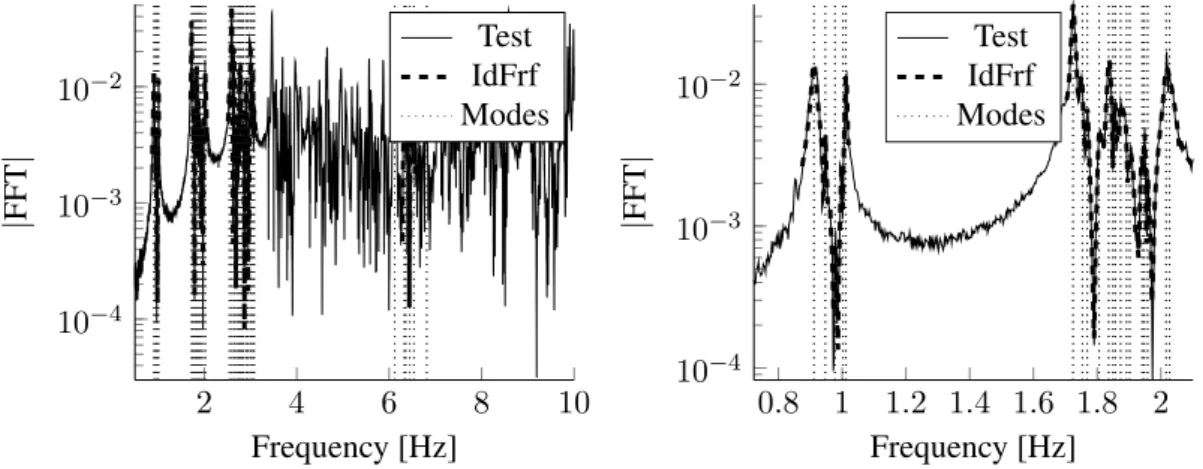
From the transient drop response, frequency response functions (FRF) can be estimated and are shown in figure 4. The FRF clearly shows groups of modes at low frequencies. These are simply related to span modes (first vertical bending, horizontal bending, ...), with some frequency split due to span coupling. Figure 3 shows an example of a span mode. For the first group of modes (vertical bending), one thus finds 6 modes associated with the 6 spans of the test catenary. Above 5 Hz, the frequency separation between mode groups becomes too small to allow a clear separation.
Figure 3. Vertical bending mode of the fourth span. 2 4 6 8 10 10−4 10−3 10−2 Frequency [Hz] |FFT | Test IdFrf Modes 0.8 1 1.2 1.4 1.6 1.8 2 10−4 10−3 10−2 Frequency [Hz] |FFT | Test IdFrf Modes
Figure 4. Complex mode identification (left) and a zoom on the two first groups (right).
The extraction of damping values from FRF is an identification step and the non-linear fre-quency domain output error method, explained by Balmes (1996), is used. An example of iden-tification is shown in figure 4. In the ideniden-tification, complex modes are used but, as damping is low, these are close to normal modes and the values can be used in modelling Balmes (1997).
For a robust identification, five points inside the −3dB band are considered good practice. For a damping of ζ = 0.5% at the frequency f = 0.9Hz of the first modes, a measurement time of 555s would be needed. Since the damping is even lower and longer signals would require maintained excitation with a shaker, there is a significant uncertainty on the damping for low frequencies.
At higher frequencies, figure 4 shows that damping remains low even though the strong modal density makes identification more difficult. Selected modes around 6 Hz were thus retained for later comparison.
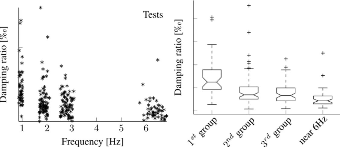
Figure 5 groups all the relevant tests and shows the dispersion for the three first groups of modes thanks to a box plot. The variability of identified damping decreases with frequency as expected. Moreover, outliers (dots of of figure 5 right) always correspond to obvious over-evaluation of the damping. Damping ratio is notably below 1% for all the frequency range observed. There is a slight decrease for the first 3 groups of modes. Then, although only the band around 6Hz was analyzed in detail, the measured responses do not show a damping variation at higher frequencies. Cremer et al. (2005) gives values of loss factors (for low damping the loss factor is equal to twice the damping ratio) for copper and bronze (that is assimilated to brass) that are close to the values observed here. This indicates that the major damping contribution is material damping, while structural effects, if present, are limited to the very low frequencies.
3 DAMPING MODELS
Damping model has always been a critical subject in problems involving vibrations. A number of models have been developed and a summary can be found in Gaul (1999). Two damping models will be compared in the following.
1 2 3 4 5 6 Tests Frequency [Hz] Damping ratio [‰] 1st group 2nd group 3rd group near 6Hz Damping ratio [‰]
Figure 5. Identified damping ratio of all tests (left) and associated box-plot (right).
3.1 Rayleigh
Without any experimental data, Rayleigh damping (also called proportional or classical damping) is typically used. It is a viscous damping proportional to the mass and stiffness matrices.
[C] = αe[K] + βe[M ] . (1)
Viscous damping is the only analytical dissipation model that is linear. It is thus needed for the sake of computation time. The piecewise Rayleigh model developed by Caughey (1960) has been introduced in OSCAR by Massat (2007), giving more flexibility to control the model but also more parameters to determine. The four elements of the catenary structure, namely the contact (CW) and messenger wires (MW), the dropper (drop) and the steady arm (SA) have thus their own contribution thanks to two coefficients each in equation 1.
0 2 4 6 8 0 2 4 6 8 10 frequency [Hz] Damping ratio [‰] Identified CW MW
Figure 6. Example of identified damping ratio on a mass drop simulation using arbitrary Rayleigh coefficients.
Figure 6 shows an example of damping identification on a simulation of a mass drop with αCW = 10−4, αM W = 5 · 10−5, βCW = 0.1, βM W = 0.05 and all the four other coefficients
fixed to 0. It appears that the modes identified correspond only with energy dissipated in CW and MW. Consequently, the only coefficients that can be set from measurements are those of CW and MW. Figure 7 compares the new fitted damping with the reference and identified damping. The difference with reference damping particularly large in the medium frequency range.
1st group 2nd group 3rd group near 6Hz Damping ratio [‰] Reference Rayleigh Rayleigh Rayleigh+Modal 10 20 30 40 50 Frequency [Hz] Damping ratio [‰] Reference Rayleigh Rayleigh Rayleigh+Modal
Figure 7. Comparison of identified (box-plot), reference (solid), Rayleigh (dashed) and Rayleigh+Modal (asterisk) damping ratio.
3.2 Rayleigh+modal
Bianchi et al. (2010) have shown that using a combined modal and Rayleigh damping respectively for low and high frequencies allows a more flexible representation of the catenary damping. The method consists in fixing the modal damping ratio found by identification and compensate the linear Rayleigh damping for some of the first modes.
Fixing the exact identified damping using modal damping is not relevant for a few reasons. First, the uncertainty on identification of low frequency is very high compared to the damping value. Secondly, one can not easily associate a measured mode with a computed one. Finally, the aim of this study is to have a damping configuration as generic as possible for a use in a large range of catenary type.
The choice was thus to fix the same modal damping for every modes in a group for the first two groups, namely the median damping identified. Figure 7 shows in asterisk the chosen damping against frequency.
4 DROPPER AND STEADY ARM DAMPING
Setting the dropper damping to zero introduces high frequency oscillations at the dropper where the mass is dropped. This numerical problem can be solved by setting the stiffness proportional damping αdropto a non-null value. In practice, there is no influence on dynamic simulations as
long as its value is small. Figure 8 shows the evolution of the maximum compensation force in the dropper against αdrop in a mid-span dropper for a usual configuration. A transition zone
is observed between 10−4 and 10−2, after which the dropper is locked by a too high dynamic stiffness. The numerical oscillation dissipates quicker for higher damping. In the following, αdrop
will thus be set to 10−5.
The steady arm, modelled as either a bar or a beam, does not dissipate any energy. One could still assume that friction exists in joints. A damping on the rotation of the steady arm can thus be introduced via a vertical damping at the claw linking the steady arm to the contact wire, under the small displacement assumption. Figure 9 shows the resulting identified damping on the simulation with the previously chosen Rayleigh coefficients and an additional vertical damping on steady arms. This contribution increases damping after the second group of modes (around 2Hz) and its impact decreases with frequency (no difference visible after 12Hz).
This damping model can thus not be used to explain the observed decrease in damping of the first three modes groups seen in figure 5. Steady arm damping will thus be set to zero.
10−9 10−7 10−5 10−3 10−1
αdrop
F
orce
[N]
Figure 8. Maximum dropper compensation force against αdrop
0 2 4 6 Frequency [Hz] Damping ratio [‰] Rayleigh theoretical Rayleigh Identified
Rayleigh+SA damp Identified
Figure 9. Comparison between identified damping ratio for simulations with Rayleigh only (asterisk) and Rayleigh with vertical dampers at steady arms (circle).
5 RESULTS
Two damping models were finally considered, the first with only Rayleigh on contact and messen-ger wires, the second with modal damping on the two first groups of modes with a compensation of Rayleigh damping at these modes. Results are observed by simulation of a mass drop and compared with measurements and with the reference Rayleigh model. The impact on a typical pantograph-catenary interaction is then observed thanks to commonly used criteria to compare models with measurements.
5.1 Mass drop
Figure 10 shows the velocity of the contact wire where a mass of 40kg is dropped in two time intervals. The first observation is that Rayleigh and Rayleigh+Modal models are exactly the same. The damping variation between the two models has thus no influence. The velocity of reference Rayleigh model is smoothed as expected by the high damping applied in medium frequency range. Tests show that the signal effectively contains energy in the medium frequency domain and val-idates the new Rayleigh model in this frequency range. The second part of the figure focuses on residual vibrations and shows that low-frequency damping of the reference is lightly too small and validates the one chosen in the new Rayleigh model.
0 0.05 0.1 0.15 0.2 0.25 0.3 0.35 0.4 0.45 0.5 0.55 0.6 0 0.5 1 Time [s] V elocity [m/s] Reference Rayleigh Rayleigh Rayleigh+Modal Measure 252 254 256 258 260 262 264 266 268 270 272 274 −5 0 5 ·10−2 Time [s] V elocity [m/s] Reference Rayleigh Rayleigh Rayleigh+Modal Measure
Figure 10. Vertical velocity of the contact wire where the mass is dropped for initial waves and residual vibration.
5.2 Dynamic pantograph-catenary simulation
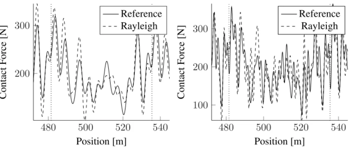
In a simulation of contact force at the nominal speed of the catenary, one observes that catenary damping has a lighter impact on the front pantograph than on the trailing one. The second panto-graph will thus be observed. Figure 11 shows the computed contact force filtered at two different frequencies, 20Hz and 50Hz The impact of damping change is clearly visible, on both of them.
Time-signal comparison is difficult. That is why scalar criteria are commonly used for compar-ison. Table 5.2 groups such criteria. The coefficients of variation of the contact force filtered at 20Hz or 50Hz cumulate informations at low and medium frequencies and do not allow to under-stand the variations observed. Root Mean Square values (RMS) inside frequency bands give more informations. One particularly observes that there is no impact for the front pantograph under 5Hz. Moreover, the RMS between 20 and 50Hz increases significantly for the rear pantograph, as expected.
Table 1. Usual contact force criteria Damping model Pantograph σ(F c)/F cm 20Hz σ(F c)/F cm 50Hz RMS* ]0 − 5] Hz RMS [5 − 20] Hz RMS [20 − 50] Hz Initial front 0.33 0.38 36.3 34.0 26.0 Updated front 0.30 0.37 36.3 29.6 29.7 Initial rear 0.23 0.28 33.6 37.0 32.9 Updated rear 0.26 0.33 33.0 41.0 42.5
480 500 520 540 200 300 Position [m] Contact F orce [N] Reference Rayleigh 480 500 520 540 100 200 300 Position [m] Contact F orce [N] Reference Rayleigh
Figure 11. Contact force of the trailing pantograph over one span filtered at 20 Hz (left) and 50 Hz (right).
6 CONCLUSIONS
Catenary damping has long been used for tuning the dynamical interaction model. The tests car-ried out on a real catenary have been exploited to estimate the catenary damping independently to the pantograph. It appeared that the very low damping observed corresponds to the hysteresis damping. The identified ratio can thus be used in any other catenary type composed of the same materials. The new damping has been validated by simulating the tests. Its impact on contact force simulation is not negligible, especially when medium frequency range is observed (over 5 Hz).
This study clearly indicates the importance of frequencies above the 20Hz fixed by standard EN50318. Current contact force measurement procedures have not been validated at higher fre-quencies and the use of lumped mass pantograph representations may no longer be relevant. It also seems that working at higher frequencies may help finding a better correlation between contact loss and arc formation.
REFERENCES
Balmes, E. 1996. Frequency domain identification of structural dynamics using the pole/residue parametrization. IMAC.
Balmes, E. 1997. New Results on the Identification of Normal Modes From Experimental Complex Modes. Mechanical Systems and Signal Processing, 11:229–243.
Bianchi, J.-P., E. Balmes, A. Bobillot, and G. Vermot des Roches 2010. Using modal damping for full model transient analysis . Application to pantograph / catenary vibration . ISMA, Pp. 1167–1180.
Bruni, S., J. Ambrosio, A. Carnicero, Y. H. Cho, L. Finner, M. Ikeda, S. Y. Kwon, J.-P. Massat, S. Stichel, M. Tur, and W. Zhang 2014. The results of the pantograph - catenary interaction benchmark. Vehicle System Dynamics, Pp. 1–24.
Caughey, T. K. 1960. Classical Normal Modes in Damped Linear Dynamic Systems. Journal of Applied Mechanics, 27(6):583–588.
Cremer, L., M. Heckl, and B. a. T. Petersson 2005. Structure-borne sound: Structural vibrations and sound radiation at audio frequencies, 3 edition. Springer-Verlag Berlin Heidelberg. Gaul, L. 1999. Description of damping and applications. In Modal Analysis and Testing, J. Silva
and N. Maia, eds., volume 363 of NATO Science Series, Pp. 409–440. Springer Netherlands. Massat, J.-P. 2007. Mod´elisation du comportement dynamique du couple pantographe-cat´enaire.