Econometric Models of Student Loan Repayment in Canada

Texte intégral

(1)2003s-68. Econometric Models of Student Loan Repayment in Canada Marie Connolly, Claude Montmarquette, Ali Béjaoui. Série Scientifique Scientific Series. Montréal Décembre 2003. © 2003 Marie Connolly, Claude Montmarquette, Ali Béjaoui. Tous droits réservés. All rights reserved. Reproduction partielle permise avec citation du document source, incluant la notice ©. Short sections may be quoted without explicit permission, if full credit, including © notice, is given to the source..

(2) CIRANO Le CIRANO est un organisme sans but lucratif constitué en vertu de la Loi des compagnies du Québec. Le financement de son infrastructure et de ses activités de recherche provient des cotisations de ses organisationsmembres, d’une subvention d’infrastructure du ministère de la Recherche, de la Science et de la Technologie, de même que des subventions et mandats obtenus par ses équipes de recherche. CIRANO is a private non-profit organization incorporated under the Québec Companies Act. Its infrastructure and research activities are funded through fees paid by member organizations, an infrastructure grant from the Ministère de la Recherche, de la Science et de la Technologie, and grants and research mandates obtained by its research teams. Les organisations-partenaires / The Partner Organizations PARTENAIRE MAJEUR . Ministère du développement économique et régional [MDER] PARTENAIRES . Alcan inc. . Axa Canada . Banque du Canada . Banque Laurentienne du Canada . Banque Nationale du Canada . Banque Royale du Canada . Bell Canada . BMO Groupe Financier . Bombardier . Bourse de Montréal . Développement des ressources humaines Canada [DRHC] . Fédération des caisses Desjardins du Québec . Gaz Métropolitain . Hydro-Québec . Industrie Canada . Ministère des Finances [MF] . Pratt & Whitney Canada Inc. . Raymond Chabot Grant Thornton . Ville de Montréal . École Polytechnique de Montréal . HEC Montréal . Université Concordia . Université de Montréal . Université du Québec à Montréal . Université Laval . Université McGill ASSOCIE A : . Institut de Finance Mathématique de Montréal (IFM2) . Laboratoires universitaires Bell Canada . Réseau de calcul et de modélisation mathématique [RCM2] . Réseau de centres d’excellence MITACS (Les mathématiques des technologies de l’information et des systèmes complexes) Les cahiers de la série scientifique (CS) visent à rendre accessibles des résultats de recherche effectuée au CIRANO afin de susciter échanges et commentaires. Ces cahiers sont écrits dans le style des publications scientifiques. Les idées et les opinions émises sont sous l’unique responsabilité des auteurs et ne représentent pas nécessairement les positions du CIRANO ou de ses partenaires. This paper presents research carried out at CIRANO and aims at encouraging discussion and comment. The observations and viewpoints expressed are the sole responsibility of the authors. They do not necessarily represent positions of CIRANO or its partners.. ISSN 1198-8177.

(3) Econometric Models of Student Loan Repayment in Canada* Marie Connolly†, Claude Montmarquette‡, Ali Béjaoui§ Résumé / Abstract Six mois après avoir mis fin à leurs études, complétées avec succès ou non, les ex-étudiants sont tenus de rembourser leurs prêts d’études. Une majorité d’entre eux rembourseront la totalité de leurs prêts sur une période de 10 ans. D’autres connaîtront des difficultés à respecter leur engagement. Dans cette étude, nous profitons d’une base exceptionnelle de données individuelles sur les prêts d’études au Canada pour étudier les déterminants des remboursements ou non des prêts et la durée avant le remboursement complet. Les résultats économétriques montrent l’importance de terminer ses études dans les temps requis à la fois pour éviter de faire défaut et aussi pour accélérer la période de remboursement. Une politique à envisager serait de gommer une partie des prêts lorsque l’étudiant complète ses études dans les temps requis. L’autre résultat est que le programme du report des intérêts n’a pas semblé très efficace pour faciliter le remboursement des prêts d’études pour la cohorte 1990-91 étudiée. Finalement, un programme trop généreux de prêts d’études sans mise en garde sur les risques encourus par les étudiants d’investir dans certains programmes, notamment ceux opérés par le secteur privé, a des effets importants non seulement sur la pérennité du programme des prêts, mais aussi sur les mauvaises décisions de la part des étudiants dans leur choix d’études. Mots clés : prêts d’études, remboursement, faillite Six months after a student ceases being enrolled full-time in an educational institution, a loan contracted with the Canada student loans program is said to be consolidated and its repayment is expected. Many ex-students will repay their loan in total (capital and interest) within a ten-year period. However, a non-negligible proportion of borrowers will experience difficulty in the repayment of their loans. We are able to shed a new light on these issues because we have access to unique data to estimate econometric models of the determinants of interest relief and claims (defaults) as well as duration models for the repayment of student loans. We found that finishing the program supported by a loan is essential to avoiding default. Therefore, it may be worth considering policies that will reward anyone who completes his or her program. On the other hand, too much flexibility in access to loans might encourage experiments by students that could turn disastrous for the student and the national loan program. A loan program should also come with some information on the risk involved for the student before he or she invests in a particular field or program. One particular concern is the relatively high level of default for students attending private schools. Relatively easy access to loans could be an invitation for private institutions to capitalize on that fact with various educational programs having little bearing on the reality of the labour market. Eventually serious institutions will establish a reputation, but for some students it will be too late. Another result concerns the interest relief measure that seems not to have played its role of helping the 1990-91 cohort of students to pass through difficult times. Keywords: student loans, reimbursement, default Codes JEL : I121, I128; C35. * We are grateful to Nathalie Viennot-Briot for her assistance and to the Socio-Economic Analysis Group of the Canada Student Loans Program, HRDC for help and comments. Any errors or omissions are our sole responsibility. † CIRANO and Department of Economics, Princeton University ‡ CIRANO and Department of Economics, University of Montreal, email: claude.montmarquette@cirano.qc.ca. § Senior Analyst, Socio-Economic Analysis Group Canada Student Loans Program, HRDC..

(4) 1. Introduction In a knowledge based economy, investment in human capital is a key determinant of economic growth. Globalization will accentuate the competitiveness between economies and therefore, to maintain our standard of living, many believe that a substantial amount of our collective resources should be devoted to higher education. One policy to achieve this goal is to facilitate access to higher education to anyone, regardless of his or her financial situation. Investments in human capital are different from other types of investment in that they cannot be backed by material collateral. Unlike investments in machinery or real estate, human capital has nothing tangible to offer to the lending institution in case of default. Thus, the capital market is an imperfect institution when it comes to offering loans to students. The Canada Student Loans Program (CSLP) provides the necessary loans to students with demonstrated need. Loans issued, from the creation of the CSLP in 1964 up to August 1995, were granted under a program which required the government to cover the entire cost of the loan. Loans that were three or more months in arrears were transferred to the federal government, which then reimbursed the lender for the defaulted loan. From August 1995 to March 1, 2001, the CSLP backed loans made by financial institutions through a risk-sharing agreement. Now all loans come directly from the Government of Canada through the National Student Loans Service Centre (NSLSC). In the fiscal year 1989–1990 the CSLP had 2,839.9 million dollars in its portfolio, as a total of both loans in study and loans in repayment. By 1995–1996, that amount had doubled to $5,821.4 million and, by 1998–1999, it had more than tripled to a value of $8,816.9 million. For students of the 1990–1991 cohort, average indebtedness, for all types of learning institutions, was $5,834. That number went up to $9,346 in 1998–1999, for a total of 358,931 students with loans. Over the same period, the average indebtedness for university students went from $8,259 to $11,900. 1. 1. More descriptive statistics and institutional details concerning Canada student loans data can be found in Plager. and Chen (1999)..

(5) Six months after a student ceases being enrolled full-time in an educational institution, a loan contracted with the Canada student loans program is said to be consolidated and its repayment is expected. Many ex-students will repay their loan in total (capital and interest) within a ten-year period. However, a non-negligible proportion of borrowers will experience difficulty in the repayment of their loans. The CSLP includes various measures to help them. One of them is the interest relief option. An ex-student using this program sees his or her monthly payment of interest put on hold for a certain period of time. The CSLP is responsible for paying interest to the lending institutions, but the interest is added to the loan to be repaid by the student. The value of the interest relief afforded by this system went from $4.2 million for the loan year 1987–1988 to $36.1 million in 1997 to $67.4 million in 1998–1999. In the meantime, the number of recipients went from 23,136 in 1987–1988 to 148,488 in 1998–1999. Another reality of the educational loan system is those ex-students who simply cannot repay. A loan is deemed in default if it is in arrears for three or more months. In 1990–1991, 20.7 per cent of loans were in default. That proportion reached a peak in 1994–1995 at 29.8 per cent, and then went down to 24.9 per cent in 1998–1999. Furthermore, for the 1998–1999 consolidation cohort, the default rate of former students was 12.9 per cent of students from universities, 26.0 per cent of those from community colleges, and 43.6 per cent of those from private institutions. Until 1994 banks simply had to claim loans in default from the CSLP, which would then try to recover the funds from the student. Between 1994 and 2001, the financial institutions issuing loans had a risk-sharing agreement with the CSLP, under which they had to recover the loans that went into claims in return for a government payment of five percent of the value of the loans going into repayment. Since 2001, the new NSLSC is responsible for all phases of the program. Although the government is able to recover a portion of the loans that go into default after a claim by the bank, some of the borrowers simply never repay. High levels of default are a threat to the viability of the system. Since the CSLP is constantly in deficit, it is actually subsidizing higher education when in fact it was created to correct the imperfect capital market. With indebtedness and the number of students who require financial aid growing larger and larger, the health of the whole system is at stake. It is thus crucial to. 2.

(6) understand the determinants of loan repayment and default. This paper studies those determinants, as well as the probability of using the interest relief option. We are able to shed a new light on this issue because we have access to unique data through Human Resources and Development Canada (HRDC). We use this data to estimate econometric models of the determinants of interest relief and claims (defaults) as well as duration models for the repayment of student loans. In the next section we present the data used in these analyses and some descriptive statistics. In section 3 we discuss the simultaneous determinants of an individual’s resorting to the interest relief option and claims. In section 4 we look at a simple duration model for repayment of student loans. We summarize the results and discuss policy issues in a concluding section.. 2. The data and some descriptive statistics The data set used in this paper consists of information about the consolidation cohort of 1990–91.2 After cleaning the files, we were left with 55,648 observations. 77.1 per cent of the students never went on interest relief or defaulted. The proportion of students defaulting on their payments, whether or not they used interest relief is 13.2 per cent. Looking at Figure 1 gives us a good general description of the situation. 1990-91 Cohort 55,648 students Breakdown of students using interest relief and/or defaulting. 10.6%. 2.6%. 9.7% Never using interest relief, No default Using interest relief, No default Using interest relief, Default. 77.1%. Figure 1 2. Consolidation occurs six months after the end of the studies, so the data we have here covers individuals who consolidated their loans during the years 1990–1991.. 3.

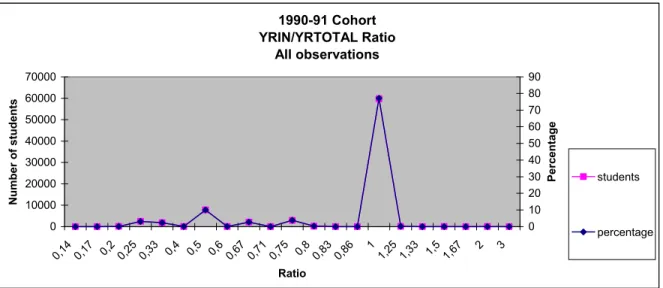
(7) The data did not include a variable for graduation, or whether or not students successfully completed their programs or quit before completion. In order to get an idea of the graduation rate and the impact of graduation on the reimbursement of loans, we create a variable for the ratio of the years of study in the last degree divided by the number of years normally required to complete the program. Although this variable is not a perfect substitute for a graduation indicator, we can speculate that an individual having a ratio lower than one probably didn’t complete the degree. If the ratio is one or more, it might have been successfully completed. As shows in Figure 2, about 77 per cent of the students had a ratio of 1, while the remaining 23 per cent had a ratio under one.. 90 80 70 60 50 40 30 20 10 0. Number of students. 70000 60000 50000 40000 30000 20000 10000. students. percentage. 3. 2. 1 1, 25 1, 33 1, 5 1, 67. 0, 14 0, 17 0, 2 0, 25 0, 33 0, 4 0, 5 0, 6 0, 67 0, 71 0, 75 0, 8 0, 83 0, 86. 0. Percentage. 1990-91 Cohort YRIN/YRTOTAL Ratio All observations. Ratio. Figure 2. 3. The determinants of interest relief options and claims The interest relief option was implemented to help students with the repayment of their loan when they go through a difficult financial period. It is important for the CSLP to understand whether that measure meets its goal—whether it is used for the right purpose. To achieve this, we need to understand the determinants of the probability of a student resorting to the interest. 4.

(8) relief option. However, to what extent does frequent resorting to the interest relief option signal inherent difficulties in loan repayment that could lead the student to default? To address this issue, we have to know the factors affecting the probability of a student having a claim, with, among other explanatory variables, the number of interest relief periods used. Both probabilities will be estimated jointly. 3.1 A joint model of interest relief and claims To analyse what influences the probability of a student using the interest relief option and going on to default, we need to estimate the parameters of two equations simultaneously. This is because we explain the probability of claims with the number of interest relief periods, but the probabilistic latent variable corresponding to this number is also a variable explained by independent variables. What is the probability that a student never resorts to the interest relief option or resorts to it only once, twice, three times,.…,? To answer this question, an ordered probit explaining the number of interest relief periods using a series of explanatory variables will be used. To explain the probability of having a claim with the same set of explanatory variables, plus dummy variables for the number of interest relief periods, a probit model of claims will be jointly estimated with the ordered probit for interest relief periods. The identification of the parameters of the complete model is a tenuous exercise considering the complexity of the model. There are no obvious exclusion restriction and we strongly rely on the non-linearity of the model to ensure identification. We are comforted by the fact that in the process of estimating the model, the likelihood function has converged with different initial values for the parameters. The probit specification for the probability of a claim is the following:. CLAIM*i = X i β + δ1D1i + δ 2 D2i + δ 3 D3i + δ 4 D4i + δ 5 D5i + δ 6 D6i + η I . CLAIM*i is a latent variable. It is the utility derived by having a claim. It is not observed. What is observed, however, is whether or not the borrower has used a claim. Thus, we define CLAIM such as:. 5.

(9) CLAIM i. = 1 if CLAIM i * > 0, that is if the utility of a claim is positive, = 0 otherwise,. where, X i is a vector of exogenous variables defined below.. Dji are dummy variables related to the number of interest relief periods, NBIRi , used by i . Thus,. D1I = 1 if NBIR I = 1 and. D1I = 0 otherwise,. D2 I = 1 if NBIR I = 2 and. D2 I = 0 otherwise,. D3 I = 1 if NBIR I = 3 and. D3 I = 0 otherwise,. D4 I = 1 if NBIR I = 4 and. D4 I = 0 otherwise,. D5 I = 1 if NBIR I = 5 and. D5 I = 0 otherwise,. D6 I = 1 if NBIR I = 6 or more an d. D6 I = 0 otherwise.. The β and δ s are parameters to be estimated. Each estimated parameter gives us the effect of a specific variable on the latent utility variable CLAIM i * . We can obtain the effect of a specific variable on the probability of having a claim by the appropriate computations. The ordered probit specification for the latent variable, NBIR i * (the utility of interest relief), is: NBIR i * = X i γ + ε i , where. X i is a vector of exogenous variables defined below. The observed variable corresponding to the latent variable is NBIRi, the number of interest relief periods, and is defined according to five µ thresholds:. 6.

(10) NBIR i = 0 if NBIR i * ≤ 0 = 1 if 0 < NBIR i * ≤ µ1, = 2 if µ1 < NBIR i * ≤ µ 2 , = 3 if µ 2 < NBIR i * ≤ µ3 , = 4 if µ3 < NBIR i * ≤ µ 4 , = 5 if µ 4 < NBIR i * ≤ µ5 , = 6 + if µ5 < NBIR i *.. In words, for example, NBIR I = 0 if NBIR i * ≤ 0 , simply means that individual i does not resort to a single period of interest relief if the utility of doing so is nonpositive. Note that. µ1 > µ 2 > ..... > µ 5 is a vector of parameters to be estimated. The errors for those equations follow a normal bivariate distribution:. η i ε i ~ NB(0,0,1,1, ρ ) with zero means, unit variances and a correlation coefficient ρ . In Table 1, the vector of exogenous variables X is defined.. 7.

(11) Table 1 The exogenous variables Variable name. Definition. Weeks. Total number of accumulated weeks of study. Amount borrowed. Natural log of the total amount borrowed. Weeks of study * amount. Number of weeks times the amount borrowed. Age. Age as of September of the consolidation year. Years of study/ years required in Constructed variable, it is the ratio of the number of actual years of study in the last program certificate of loan to the number of years normally required to complete the program. A ratio lower than one suggests that the student did not finish his program, hence did not graduate. Female. Dummy = 1 if female, =0 if male. Private institution. Dummy =1 if private institution, =0 if public institution. Amount * private. Amount borrowed times the private institution dummy. Married. Dummy=1 if marital status is married, =0 if not married. Fields of study. Ten dummy variables, = 1 if it’s the discipline of the final degree, =0 if it isn’t. Possible fields: business/administration, agriculture, arts/science, community service/education, dentistry, engineering/technology, health sciences, law, medicine, trades and theology (used here as the reference variable). Amount * dentistry. Amount borrowed times the dentistry dummy. Amount * health sciences. Amount borrowed times the health sciences dummy. Amount * law. Amount borrowed times the law dummy. Levels of study. Three dummy variables, =1 if it’s the level of study of the student. Possible levels: non-degree, undergraduate, masters and doctoral (used here as reference). Province of study. Nine dummy variables, =1 if it’s the province of issue of the last loan certificate. Possible provinces: Alberta, British Columbia, Manitoba, New Brunswick, Newfoundland, Nova Scotia, Ontario, Prince Edward Island, Saskatchewan and Yukon (used here as reference). 8.

(12) 3.2 The estimation results. The joint “claim” - “interest relief period” model has been estimated by maximum likelihood programmed in Gauss (see the detailed likelihood function in the Appendix). The results are reported in Table 2. Coefficient estimates of the number of weeks of study are negative, while those associated with the amount borrowed and the interaction variable “weeks times amount” are positive. We can see that an increase in the number of weeks of study decreases the probability of claims and of resorting to large numbers (6+) of interest relief periods, owing to the impact of the direct coefficient, but that these probabilities increase with an increase in the “weeks*amount-borrowed” interaction variable.3 Thus, studying more helps ward off claims and interest relief, probably because of completion of the program or a more advanced degree; but at the same time, studying for a longer period may also mean borrowing more, and hence having more difficulty repaying.. 3. A positive coefficient increases the probability of a claim with an increase in the value of the corresponding. variable. In the case of an ordered probit (the interest relief equation) this one-to-one relation is only valid at the extremes: no interest relief period and 6+ interest relief periods. An increase in the value of a variable with a positive coefficient estimate increases (decreases) the probability of resorting to six or more interest relief periods (no interest relief period). Between these categories, the final effect has to be individually computed.. 9.

(13) Table 2 Results of the ¨claim-interest relief period¨ joint estimation Independent variables. Claims Interest relief beta estimates gamma estimates. Constant Number of weeks of study Amount borrowed (ln) Weeks of study * amount Age Years of study/Years required in program. Male Female Private institution Public institution Amount * private institution dummy Married Not married. -1,5197 (-6,406). -1,4327 (-6,045). -0,1666 (-9,808). -0,1187 (-8,056). 0,4115 (31,600). 0,3965 (30,904). 0,1767 (11,342) 0,1504 (24,360) -0,4714 (-11,199) ref.. 0,1328 (9,781) 0,1338 (23,447) -0,2935 (-10,083) ref.. 0,0226 (1,598). 0,047 (3,588). 0,2786 (9,553). 0,2521 (8,832). ref. -0,0609 (-5,803) -0,0309 (-1,430) ref.. ref. -0,0544 (-5,236) -0,0379 (-1,788) ref.. Independent variables Engineering/Techn ology. Agriculture Arts/science Community Service/Education Dentistry Yukon. Interest relief Gamma estimates. 0,0546 (0,773). 0,0728 (1,053). -0,0982 (-1,245). -0,091 (-1,184). 0,4431 (4,316. 0,3366 (3,398). -1,2072 (-10,158) 0,469 (6,494) ref.. -1,2352 (-9,947) 0,3661 (5,312) ref.. -0,0625 (-4,733). -0,0617 (-5,972). -0,0441 (-3,820). -0,0491 (-4,426). -0,0703 (-5,944). -0,0561 (-4,951). 0,6924 (5,501) 0,3329 (2,718). 0,5086 (4,085) 0,234 (1,897). 0,0128 (0,102) ref.. 0,0106 (0,084) ref.. -0,0412 (-0,227) 0,1627 (0,893) 0,0999. -0,039 (-0,205) 0,1111 (0,583) 0,0899. Health Sciences Law Medicine Trades Theology Amount borrowed * Dentistry dummy Amount * Health Sciences dummy Amount * Law dummy. Level of study Non-degree Undergraduate. Fields of study Business/Administ ration. Claims Beta estimates. Masters 0,3024 (4,379) 0,033 (0,396) 0,5436 (7,820) 0,0602 (0,858) 0,1377 (0,938). 0,2694 (3,994) 0,0618 (0,760) 0,47 (6,980) 0,0452 (0,658) 0,162 (1,283). ref.. ref.. Doctorate Province of study Alberta British Columbia Manitoba. 10.

(14) Number of IR periods Zero One. ρ. (correlation coefficient) ref.. -. -0,0863 (-1,227). -. -0,3501 (-4,954). -. -0,5392 (-7,211). -. -0,6838 (-8,012). -. -0,8403 (-8,377) six or more -1,3161 (-14,754) Number of observations: 55648 Log-likelihood: -58147,70816 Mean log-likelihood: -1,04492. -. Two Three Four Five. µ1 µ2 µ3 µ4 µ5. 0,9637 (53,236) -. 0,2888 (63,487) 0,5035 (81,832) 0,6852 (92,523) 0,8674 (99,933) 1,1218 (104,821). The coefficient estimates for the years of study/years required ratios are highly significant and negative, which indicates that a greater ratio lowers the probability of going into claims or using the interest relief option. Assuming that a higher ratio is associated with completion of the program and graduation, we realize how crucial it is for students to pursue their studies until the end. Students who have completed their programs have a lower risk of experiencing difficulty in repayment of their loans. This is explained by the well-known fact that a degree holder has a much better chance of finding good employment than someone who hasn’t finished his or her degree. The coefficients of the private institution dummy are all positive, which implies that attending a private school increases the probability of defaulting and using more interest relief periods. An interesting result is the one regarding the interaction variable “amount borrowed*private institution.” A negative estimate tells us that attending a private school actually decreases the probability of claims and interest relief in proportion of the amount borrowed. The effect of going to a private school then works in both directions. This mixed result may in fact capture the fact that a student from a private institution tends to borrow more. 11.

(15) because of higher tuition fees, but might in return get a good technical degree that leads to a well-paid job. Relative to the theology coefficient, the coefficients of the medicine dummy variable are all very significant and negative, so we can imagine going to medical school significantly lowers the risk of default and interest relief. Although the results for the coefficients of the field of study dummies are not very significant in general, the estimates for the cross-variables dummies of ämount and dentistry¨, ämount and health sciences¨ and ämount and law¨ are all negative and significant but one. We can conclude that studying in one of those fields actually reduces the probability of having a claim or using interest relief, in proportion with the amount borrowed. To study how using the interest relief option affects the probability of default, we cannot simply consider the coefficients associated with the different numbers of periods of interest relief, owing to the joint estimation of our two-equation model. To obtain the probability of having a claim, conditional to the number of periods of interest relief, the following formula must be used: Pr ( CLAIM = 1/NBIR = j ) =. Pr(CLAIM = 1,NBIR = j ) ; j = 0,..., 6. Pr(NBIR = j ). With the coefficients of Table 2 and with the exogenous variables taken at their mean values, the mean amount borrowed, the mean number of weeks, etc., Figure 3 shows the probabilities of having a claim, conditional on the number of periods of interest relief.. 12.

(16) Figure 3. We see that the probability of claims is very low, less than 10 per cent, when the student never uses the interest relief option. That probability rises dramatically to around 70 per cent for students with one or more periods of interest relief. Interestingly enough, that probability doesn’t vary much with the number of interest relief periods between one and six. With other variables taken at their mean values, Figure 4 shows the probability of having a claim, expressed relative to the total amount borrowed. The solid one represents the probability for public institutions and the dotted one—private institutions. We observe that the probability of a claim is strictly monotonically increasing with the amount borrowed, and that the curve for private institutions is above the one for public institutions. This tells us that the more students borrow, the more likely they are to have difficulty repaying, and that attending a private institution raises the probability of defaulting.. 13.

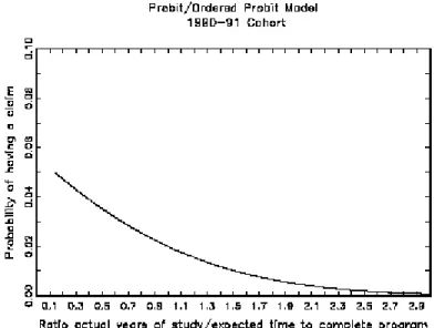
(17) Figure 4. Figure 5 represents the probability of having a claim, this time plotted against the ratio of actual years of study to the expected time needed to complete the program. This probability is strictly decreasing from 5 per cent, when the ratio is zero, to around 2 per cent with a ratio of one, to almost zero as the ratio increases. Thus, the higher the ratio, and so hypothetically the higher the probability of graduating, the lower the probability of a student defaulting.. Figure 5. 14.

(18) We turn next to the determinants of the probability of using the interest relief option a certain number of times. Table 3 presents some simulation results by sub-groups of the explanatory variables. Using the coefficient estimates of Table 2, these simulations were done by calculating the probability of using the interest relief option for each possible value of the variable NBIR from none to six or more, for each individual in the database. The sample was then separated into sub-groups according to the characteristics of the individuals. For example, the group was divided between males and females. The probabilities shown in the Tables are the means of the probabilities for the observations in that sub-group. The standard deviation is presented in italics. There are two ways to read these Tables. One is by line, from left to right. That way, we can observe how the probability varies for the different numbers of periods of interest relief within each sub-group. The other way is by column. By comparing two numbers in the same column, we see the difference in the probability of requiring interest relief a certain number of times for the different sub-groups. In Table 3 we can see that, for a married individual, the probability of never resorting to interest relief is 79 per cent, of resorting to it once, 7 per cent, twice, 4 per cent, and so on. If we look at the column “none“ for the different ranges of amount borrowed, we see that the probability of never using interest relief greatly diminishes with the amount borrowed, going from 90 per cent for amounts under $2,500 to 69 per cent for amounts above $12,500. As expected, students in the field of medicine have the highest probability of never using the interest relief option.. 15.

(19) Table 3 Simulation of the probability of using interest relief Cohort 1990–91 Number of interest relief periods. None. One. Two. Three. Four. Five. Six and more. Categories Married 4709. 0,78617 0,11880. 0,06877 0,02613. 0,04028 0,01881. 0,02720 0,01468. 0,02153 0,01315. 0,02185 0,01532. 0,03420 0,03423. Single 50939. 0,79885 0,11373. 0,06605 0,02608. 0,03827 0,01841. 0,02562 0,01418. 0,02012 0,01256. 0,02023 0,01445. 0,03086 0,03141. Weeks<35 11600. 0,84975 0,08323. 0,05442 0,02323. 0,02993 0,01505. 0,01919 0,01084. 0,01447 0,00903. 0,01385 0,00966. 0,01839 0,01669. 35<=Weeks<70 14246. 0,80679 0,10018. 0,06508 0,02497. 0,03732 0,01712. 0,02474 0,01285. 0,01924 0,01109. 0,01908 0,01234. 0,02774 0,02355. Weeks>=70 29802. 0,77324 0,12319. 0,07147 0,02610. 0,04230 0,01908. 0,02879 0,01507. 0,02296 0,01363. 0,02352 0,01606. 0,03773 0,03725. Amount borrowed <2500$ 10250. 0,89680 0,06794. 0,04047 0,02136. 0,02112 0,01298. 0,01301 0,00892. 0,00946 0,00712. 0,00868 0,00726. 0,01044 0,01113. 2500<=Amount<5000 18189. 0,81276 0,08626. 0,06464 0,02126. 0,03661 0,01475. 0,02401 0,01112. 0,01848 0,00961. 0,01810 0,01068. 0,02541 0,02011. 5000<=Amount<7500 9729. 0,78317 0,09298. 0,07162 0,02106. 0,04159 0,01525. 0,02782 0,01183. 0,02179 0,01047. 0,02179 0,01194. 0,03222 0,02377. 7500<=Amount<10000 5859. 0,76882 0,10211. 0,07426 0,02262. 0,04375 0,01642. 0,02961 0,01284. 0,02344 0,01146. 0,02375 0,01323. 0,03637 0,02739. 10000<=Amount<12500 4429. 0,74535 0,10427. 0,07930 0,02120. 0,04749 0,01603. 0,03255 0,01287. 0,02607 0,01175. 0,02677 0,01388. 0,04248 0,03074. 12500<=Amount 7192. 0,69440 0,14414. 0,08547 0,02577. 0,05362 0,02001. 0,03820 0,01661. 0,03175 0,01572. 0,03414 0,01955. 0,06243 0,05321. Age<25 33962. 0,82287 0,09915. 0,06091 0,02501. 0,03448 0,01699. 0,02264 0,01269. 0,01745 0,01093. 0,01716 0,01214. 0,02450 0,02339. Age>=25 21686. 0,75848 0,12470. 0,07470 0,02553. 0,04466 0,01894. 0,03064 0,01512. 0,02460 0,01380. 0,02540 0,04153 0,01642 0,03925 continued on the next page. 16.

(20) Years in program/years required<1 12714. 0,80026. 0,06526. 0,03787. 0,02539. 0,01998. 0,02015. 0,03110. 0,11848. 0,02696. 0,01905. 0,01470. 0,01305. 0,01507. 0,03352. Years in program/years required>=1 42934. 0,79704. 0,06658. 0,03862. 0,02586. 0,02031. 0,02043. 0,03115. 0,11292. 0,02583. 0,01827. 0,01409. 0,01249. 0,01437. 0,03111. Female 33359. 0,79510 0,11456. 0,06693 0,02595. 0,03889 0,01843. 0,02609 0,01425. 0,02053 0,01266. 0,02069 0,01462. 0,03176 0,03212. Male 22289. 0,80178 0,11359. 0,06531 0,02628. 0,03777 0,01848. 0,02525 0,01419. 0,01980 0,01254. 0,01988 0,01439. 0,03021 0,03098. Private Institution 25384. 0,78705 0,10675. 0,06956 0,02475. 0,04055 0,01752. 0,02723 0,01348. 0,02143 0,01189. 0,02157 0,01357. 0,03262 0,02773. Public Institution 30264. 0,80677 0,11939. 0,06353 0,02686. 0,03668 0,01903. 0,02451 0,01473. 0,01924 0,01311. 0,01936 0,01522. 0,02990 0,03459. Fields of Study Business/Administration 13112. 0,78361 0,10225. 0,07077 0,02353. 0,04127 0,01678. 0,02771 0,01294. 0,02179 0,01143. 0,02191 0,01304. 0,03295 0,02644. Agriculture 931. 0,82727 0,09723. 0,05984 0,02498. 0,03373 0,01680. 0,02208 0,01246. 0,01697 0,01067. 0,01662 0,01179. 0,02350 0,02272. Arts/science 14005. 0,75447 0,13196. 0,07492 0,02605. 0,04501 0,01960. 0,03102 0,01580. 0,02503 0,01455. 0,02601 0,01751. 0,04355 0,04341. Community Service/Education 7539. 0,82969. 0,05881. 0,03311. 0,02168. 0,01669. 0,01640. 0,02363. 0,10291. 0,02490. 0,01720. 0,01302. 0,01135. 0,01281. 0,02620. Dentistry 493. 0,89682 0,04927. 0,04163 0,01576. 0,02139 0,00959. 0,01298 0,00654. 0,00930 0,00517. 0,00836 0,00516. 0,00951 0,00726. Engineering/Technology 5181. 0,82874 0,09484. 0,05962 0,02463. 0,03353 0,01654. 0,02190 0,01223. 0,01680 0,01042. 0,01641 0,01144. 0,02301 0,02128. Health Sciences 5862. 0,87044 0,06879. 0,04909 0,02050. 0,02627 0,01288. 0,01648 0,00905. 0,01218 0,00736. 0,01137 0,00764. 0,01416 0,01207. Law 1441. 0,82982 0,06665. 0,06127 0,01710. 0,03393 0,01159. 0,02183 0,00861. 0,01649 0,00736. 0,01579 0,00809. 0,02087 0,01534. Medicine 683. 0,97453 0,02980. 0,01209 0,01146. 0,00540 0,00609. 0,00296 0,00381. 0,00194 0,00281. 0,00158 0,00149 0,00264 0,00339 continued on the next page. 17.

(21) Trades 5903. 0,74752 0,09506. 0,07951 0,01957. 0,04741 0,01472. 0,03236 0,01178. 0,02580 0,01072. 0,02635 0,01263. 0,04105 0,02765. Theology 498. 0,83551 0,08969. 0,05824 0,02209. 0,03240 0,01524. 0,02098 0,01149. 0,01598 0,00995. 0,01549 0,01111. 0,02139 0,02135. Level of Study Non-degree 31676. 0,78780 0,10695. 0,06939 0,02434. 0,04040 0,01734. 0,02711 0,01341. 0,02132 0,01189. 0,02146 0,01367. 0,03253 0,02901. Undergraduate 21985. 0,81077 0,12096. 0,06231 0,02774. 0,03594 0,01952. 0,02400 0,01502. 0,01883 0,01331. 0,01895 0,01534. 0,02920 0,03374. Masters 1855. 0,81381 0,12726. 0,06104 0,02676. 0,03510 0,01940. 0,02343 0,01530. 0,01841 0,01387. 0,01859 0,01646. 0,02961 0,04090. Ph.D. 132. 0,80311 0,18839. 0,05619 0,03489. 0,03377 0,02495. 0,02355 0,02003. 0,01938 0,01885. 0,02088 0,02390. 0,04313 0,08133. Province of Study Alberta 9606. 0,80443 0,10274. 0,06555 0,02448. 0,03765 0,01711. 0,02500 0,01305. 0,01948 0,01142. 0,01938 0,01292. 0,02851 0,02571. BC 7010. 0,76745 0,11443. 0,07365 0,02297. 0,04352 0,01716. 0,02956 0,01376. 0,02352 0,01261. 0,02402 0,01510. 0,03828 0,03763. Manitoba 3159. 0,77428 0,10367. 0,07289 0,02292. 0,04278 0,01660. 0,02888 0,01297. 0,02282 0,01158. 0,02307 0,01340. 0,03528 0,02872. New Brunswick 2889. 0,76386 0,10644. 0,07508 0,02280. 0,04443 0,01678. 0,03018 0,01324. 0,02399 0,01193. 0,02443 0,01392. 0,03803 0,03019. Newfoundland 2546. 0,69128 0,13432. 0,08708 0,02305. 0,05450 0,01851. 0,03873 0,01557. 0,03211 0,01483. 0,03440 0,01846. 0,06189 0,04889. Nova Scotia 3071. 0,71486 0,11798. 0,08432 0,02103. 0,05170 0,01673. 0,03612 0,01394. 0,02946 0,01314. 0,03095 0,01614. 0,05258 0,04103. Ontario 22520. 0,84129 0,09855. 0,05578 0,02546. 0,03112 0,01701. 0,02022 0,01259. 0,01545 0,01077. 0,01504 0,01191. 0,02111 0,02326. Prince Edward Island 523. 0,80292 0,09486. 0,06656 0,02275. 0,03814 0,01589. 0,02525 0,01210. 0,01961 0,01056. 0,01942 0,01191. 0,02811 0,02337. Saskatchewan 4269. 0,76632 0,10219. 0,07487 0,02176. 0,04414 0,01606. 0,02989 0,01269. 0,02369 0,01145. 0,02403 0,03706 0,01338 0,02941 continued on the next page. 18.

(22) Yukon 55. 0,76563 0,11191. 0,07428 0,02446. 0,04402 0,01786. 0,02994 0,01403. 0,02383 0,01257. 0,02431 0,01457. 0,03799 0,03027. Total number of observations 55648 *The numbers below the category names are the number of observations in each category. *The probabilities in the columns are the mean probability of using interest relief for the observations in that category. *The numbers in italics are the standard deviations of the probabilities for that category.. 4. A duration model for the repayment of student loans Now that we have looked at the determinants of having a claim or interest relief, we want to focus on the reimbursement itself. What characteristics make one individual repay in a shorter period of time than another? Do people tend to repay their loan quickly or slowly? How does the time spent in the reimbursement phase affect the probability of full remittance at any given time? Those are questions that can be answered through the use of an econometric duration model. A duration model provides us with a survival function, which characterizes the probability of survival in the repayment state, the time spent before total reimbursement. It is also associated with a hazard function, which gives us the rate at which a student exits the repayment phase, given that he has not already exited. Looking at the shape of the hazard rate function will tell us more about the pattern of loan repayment. A duration model can also include independent variables, which do not change the shape of the hazard but rather its vertical position. A variable that affects the duration negatively will make the hazard function shift upwards, leaving it more likely for an individual to exit the state at any given time. The data we have for durations before students repay their loans consists of 53,574 observations for the 1990–91 cohort. The duration variable is defined as follows: the time in months before total loan repayment by the student starting at consolidation date. The variable is censored if, at the time the database was constructed, the student was still in repayment phase. There are 16,887 censored observations, or 32 per cent of the total.. 19.

(23) A loan deemed in default is not considered repaid, except if it is recovered by a collection agency or the government. We include dummy variables for claims and interest relief in the regression, thus indicating a student who experiences financial difficulties. Thus, these variables are treated here as exogenous. Three reasons justify our choice. First, a ten-year period is relatively short for the repayment of student loans, therefore we consider this duration model an investigative exercise. Second, we do not have strong instruments to use for the claim and interest relief variables. Finally, a joint estimation of ¨claim-interest relief-duration of repayment of loans¨ will impose a lognormal hazard rate to form a trivariate normal distribution with the probit for claims and the ordered probit for interest relief. 4.1. The duration model. We estimate a duration model with a Weibull hazard and a Gamma correction for unobserved heterogeneity. The unobserved characteristics or variables such as the individual’s motivation to find a job, health status need particular attention in duration model. The log-likelihood function estimated for this model is:. ln( L) =. [(. ∑ δ ln λ i p (λ i t i ). i uncensored. p −1. ) − ln(1 + θ (λ i t i) )] p. −1. θ + ∑ ln 1+θ (λ i t i ) p  ,   all. where. (. ). ' λ i = exp − β xi ,. and X I = (one, correction dummy, weeks of study, amount borrowed, age, years of study/years required, interest relief dummy, claims dummy, sex, type of institution [private dummy], marital status, field of study dummies, level of study dummies, province dummies. See Table 1 for details). The δ coefficient is equal to one for the observations on individuals who exited the repayment phase (the uncensored observations). About 10% of individuals repaid their loan immediately when the consolidation period started. Most likely, for these individuals the loan was not essential to their pursuit of studies. Since we take the natural log of the duration variable. 20.

(24) t, we add 0.00001 to the observations for which t = 0. Those observations are then given a value of one for a correction dummy—zero otherwise. The survival function of this model is:. [. S (t ) = 1 + θ (λt ). ]. −1 p θ. and the hazard function is:. λ (t ) = λp(λt ) p −1 [S (t )]θ We will see in the results that θ is larger than zero, and thus our correction for heterogeneity is necessary. 4.2. The empirical results. The coefficients for the duration model are estimated using maximum-likelihood optimization from Gauss. The results are presented in Table 4. The graphs of the hazard functions are presented in Figure 6. Interestingly enough, when a Weibull hazard is corrected for heterogeneity, the shape of the hazard changes and is no longer strictly increasing or decreasing. We can see in Figure 6 that the hazard rate is increasing up to a certain point, close to two years, and then decreasing as the duration goes up. This shape is what we expected: The probability of fully reimbursing a loan starts at a certain level at consolidation date, then this probability goes up with time as the ex-students find employment, then get experience, a better salary, and an overall improved financial situation. After a certain time, represented by the peak in the hazard function, the probability of exit goes down, due to the fact that those individuals still in the repayment phase at that point tend to have difficulty repaying because of an underpaid job or a heavy debt load. This leads to a lower hazard rate, and that rate continues decreasing as time goes by. What this shows us is that it becomes less likely for an individual to exit the repayment spell the longer it’s been since the consolidation. While this general shape was the one expected for such a model, we would have thought that the return point in the hazard rate function, here at around two years, would be further to the right, after a longer period of time. Two years seems a short time to get rid of a student loan, especially when you consider the amounts borrowed and. 21.

(25) the advantageous interest rates. What could explain that this curve is skewed to the left? First, it could be because of the number of ex-students who reimbursed their loan in one shot at the consolidation date, or right after. These people probably didn’t really need a loan and borrowed only for a strategic reason. The second explanation for that early return point might be a phenomenon of debt aversion. Even if borrowers don’t have to repay quickly, they prefer to do so because they feel uncomfor with indebtedness.. 22.

(26) Table 4 1990–91 Cohort with correction for heterogeneity Parameters. Estimates. St. Dev.. T-stat. Constant Correction for duration=0 Duration>0. 3.7905283 -15.615480. 0.2290 0.0291. 16.552 -536.017. Number of weeks of study Amount borrowed Age Years of study/Years required Interest Relief = 1 Interest Relief = 0 Claims=1 Claims=0 Female Male Private Institution Public Institution Married Not married Fields of study Business/Administrati on Agriculture Arts/science Community service/Education Dentistry Engineering/Technolo gy. ref.. Prob.. Parameters Health Sciences 0.0000 Law 0.0000 Medicine. Estimates -0.15847428 -0.13359903 -0.54121276. St. Dev. 0.0711 0.0766 0.0850. T-stat -2.229 -1.743 -6.368. Prob. 0.0258 0.0813 0.0000. Trades. 0.0016667082 ref.. 0.0709. -0.023. 0.9813. 0.00022733234. 0.0001. 1.713. 0.0868 Theology. 3.5666063e-05 0.0051419712 -0.057888623. 0.0000 0.0011 0.0271. 16.235 4.693 -2.138. 0.0000 0.0000 Level of study 0.0325 Non-degree. 0.49476297. 0.1178. 4.199. 0.0000. 0.33129892 ref. 0.80026831 ref. 0.022118518 ref. -0.0071948043 ref. 0.093272073 ref.. 0.0174. 19.055. 2.719 0.760. 0.0066 0.4474. 35.973. 0.31718823 0.091116601 ref.. 0.1167 0.1199. 0.0222. 0.0000 Undergraduate Masters 0.0000 Doctorate. 0.0125. 1.775. 0.0197. -0.364. 0.0214. 4.363. -0.38911609 -0.081557594 -0.27710862 -0.038512236 -0.14090652 -0.094239339 -0.33227864. 0.1764 0.1768 0.1775 0.1775 0.1780 0.1777 0.1761. -2.206 -0.461 -1.561 -0.217 -0.792 -0.530 -1.887. 0.0274 0.6446 0.1184 0.8283 0.4285 0.5959 0.0592. -0.067283040. 0.0691. -0.973. 0.0759 Province of study Alberta 0.7155 British Columbia Manitoba 0.0000 New-Brunswick Newfoundland Nova Scotia Ontario 0.3304. -0.046681196. 0.0808. -0.578. 0.0047342764. 0.1814. 0.026. 0.9792. -0.013090346 -0.070939429. 0.0699 0.0705. -0.187 -1.007. 0.5634 Prince Edward Island 0.8515 Saskatchewan 0.3141 Yukon. -0.25461185 ref.. 0.1771. -1.438. 0.1506. -0.34771308 -0.10850125. 0.0905 0.0703. -3.840 -1.543. 0.0001 0.1227 P. 1.1621213. 0.0098. 118.756. 0.0000. θ. 0.50850829. 0.0284. 17.877. 0.0000. Number of observations: 53574 Log- likelihood : -175430.20596 Mean log-likelihood : -3.27454. 23.

(27) Figure 6. It is interesting to look at the signs of the estimated coefficients presented in Table 4. A negative (positive) sign means that the variable has a negative (positive) effect on the duration, and induces a shift upwards (downwards) in the hazard rate function. The coefficient associated with the correction dummies for a duration equal to zero is very large, highly significant and negative. Of course, if an observation has a value of zero for a duration, this greatly lowers its duration. But this result is interesting mostly because it shows us that there are individuals who fully reimburse their loan the minute they get out of school. Clearly, they had a loan for a financially strategic reason and not because of insufficient funds to attend school. This is part of the reality of student loans: students who get financial aid but don’t really need it. Variables having a positive coefficient include: the amount borrowed, age, the interest relief dummy, and the married dummy. It comes as no surprise that the amount borrowed has a positive and significant effect on the time before repayment. Just like the amount borrowed increased the probability of defaulting or resorting to the interest relief measure, here it increases the time spent in the repayment phase. The age variable has a positive effect too, but quite small. It is significant, but perhaps doesn’t play a major role. Same scenario for the married variable, but with a slightly larger effect. This result shows us that a married person is less likely to exit. 24.

(28) the repayment phase than an unmarried one. This is consistent with the assumption that married individuals might need to support their partners and/or children, making it more difficult for them to reimburse their student loans. Another reality of student loans we have to keep in mind is the fact that those loans generally have very low interest rates. For those who have debt from different sources, like credit card bills, car payments or mortgage payments, it might be part of a financial strategy to repay the student loan last. To avoid paying high interest on the credit cards, for example, one might fully pay their credit card bills, thus postponing payment of the student loan. Since student loans present such advantageous rates, they are often at the bottom of the priority list when it comes to paying the bills. The interest relief dummy coefficient is very significant, quite large and positive. It clearly indicates that a student who is on interest relief has a much lower hazard rate for exiting the repayment spell. Now, while the interest relief dummy is an indicator of a student in financial difficulty, there might be a simpler explanation for the strength of its impact on the hazard rate of exit. Using the interest relief option lengthens the repayment because that’s what it precisely does: help students go through a difficult period, letting them defer payments until a later date. For the claim dummy, the positive coefficient suggests that having a claim makes the duration before repayment longer, which is what we would normally expect: a student who defaults is one who has difficulty meeting his payments, and it will probably take a long time for a collection agency to collect the money owed. Looking now at the fields of study coefficients, we see that only the ones for dentistry, health sciences and medicine are significant. They are all negative and relatively large, especially the one for medicine. This comes as no surprise at all: graduating as a medical doctor or a dentist greatly lowers the duration of the repayment period. Simple to understand: they make more money on their jobs, have fewer or no financial difficulties, and so repay much faster. The other significant variables we have are business, agriculture, art and science, education and trades, all of which are positive. Individuals graduating in those fields tend to take more time to reimburse their loans, and their hazard rate is lower, compared to the reference field which is theology.. 25.

(29) If we turn now to the level of study dummies, we see that the non-degree and undergraduate variables are significant and positive. This implies that, compared to borrowers who study at the Ph.D. level, the ones with an undergraduate degree or no degree show a longer period of repayment. Another measure we can look at while analysing the results of an econometric duration model is the median time. It is defined as the length of time after which half of the students have repaid their loan, or exited the repayment phase. It is the value of duration for which the survival function equals 0.5. The median time for the 1990–91 cohort is about 41 months, or 3½ years. This tells us that half the students fully repay their loan after 3½ years. This result is certainly affected by those individuals who repaid their loan immediately at the consolidation date. Despite addressing several important questions, it would be interesting for further studies to have access to more extended databases. Other extensions could include a more complex model with time-varying covariates, such as unemployment, economic growth, or changing personal characteristics. With a longer time period, it will be worthy to address the endogeneity issue with regards to the claims and interest relief variables and to better account for those individuals repaying their loan at the consolidation date .. 5. Conclusion and policy issues This paper has benefited from access to a unique set of data for the study of patterns of student loans repayment in Canada. Billions of dollars are at sake and more than three hundred thousand students have been associated with the program in recent years. The justification for this program stems from a government policy aimed at facilitating access to higher education for all Canadians (the same applies to Québec, which has its own program) in the context of a knowledge based economy. Unlike real or financial investments, human capital investment has nothing tangible to offer to the lending institution in case of default. Thus, the capital market is an imperfect institution when it comes to offering loans to students. The Canada Student Loans Program (CSLP) is an answer and provides the necessary loans to students with demonstrated. 26.

(30) need. But investment in human capital is like any other investment—a risky enterprise. A reality of the educational loan system is that close to one ex-student in five simply cannot repay his or her loan. Many more experience difficulties in paying back their loan. High levels of default are a threat to the viability of the system. Since the CSLP is constantly in deficit, it is actually giving subsidies to higher education, when in fact it was created to correct the imperfect capital market. With indebtedness and the number of students who require financial aid growing larger and larger, the health of the whole system is at stake. It is thus crucial to understand the determinants of loan repayment and default. This paper has studied those determinants, as well as the probability of using the interest relief option, a specific measure to ease repayment of the loan when a participant goes through a period of unemployment or partial employment. Among the many results derived from our econometric models, a few are particularly interesting for policy issues. First, finishing the program supported by a loan is essential to avoiding default. Therefore, it may be worth considering policies that will reward anyone who completes his or her program. For example, by transforming part of the loan into a grant if this objective is met in due time. On the other hand, too much flexibility in access to loans might encourage experiments by students that could turn disastrous for the student and the national loan program. A loan program should also come with some information on the risk involved for the student before he or she invests in a particular field or program. Better information about the labour market is essential. One particular concern is the relatively high level of default for students attending private schools. Relatively easy access to loans could be an invitation for private institutions to capitalize on that fact with various educational programs having little bearing on the reality of the labour market. Eventually serious institutions will establish a reputation, but for some students it will be too late. The second result concerns the interest relief measure that seems not to have played its role of helping student pass through difficult times. This could explain why, recently, important modifications were brought to this program. It will be important to review this question with a new cohort. Finally, not all students needed the loan program to pursue higher education. With scarce resources, funding these windfall gains is a flaw in the program. Whether by chance, because of debt aversion, or out of a particular sense of civic duty, many participants repaid their student loans in a relatively short period of time. A. 27.

(31) policy systematically reminding the beneficiary of his own commitment to the perpetuation of the collective loan program might be useful to consider, starting two years after the loan is consolidated. More work needs to be done, however, to complete the study of patterns of loan repayment in Canada. In addition to some methodological issues raised earlier, our estimates need to be updated with new and revised data.. 28.

(32) References FINNIE, Ross and SCHWARTZ, Saul (1996), Student Loans in Canada. Past, Present, and Future, C.D. Howe Institute, Toronto, Observation 42, 162 pages. PLAGER, Laurie and CHEN, Edward, (1999), “Student debt from 1990–91 to 1995–96: An analysis of Canada Student Loan data”, Education Quarterly Review, Statistics CanadaCatalogue no. 81-003, vol 5(4), 10-28. The Canada Student Loan Program website http://www.canlearn.ca/English/csl/index.cfm. 29.

(33) Appendix Individual contributions to the likelihood function of the claim-interest relief period (probitordered probit) model are calculated using a bivariate normal distribution of the residuals,. η i ε i ~ NB(0,0,1,1, ρ ) , with a correlation coefficient of ρ . Specifically, the joint probabilities are defined as follows for all cases: ∞ -Ziγ. P(CLAIMSi=1, NBIRi=0) =. ∫ ∫ φ 2 (η i , ε i )dε i , dη i. -X i β −∞ ∞. P(CLAIMSi=1, NBIRi=1) =. ∫. ∫. P(CLAIMSi=1, NBIRi=6) =. µ 3 − Ziγ. ∫ φ (η i , ε i )dε i , dη i. 2 − X i β −δ 3 µ − Z γ 2 i. µ 4 − Zi γ. ∫ φ 2 (η i , ε i )dε i , dη i. ∫. − X i β −δ 4 µ 3 − Ziγ ∞. P(CLAIMSi=1, NBIRi=5) =. ∫ φ 2 (η i , ε i )dε i , dη i. ∫. ∞. P(CLAIMSi=1, NBIRi=4) =. µ 2 − Zi γ. − X i β −δ 2 µ1 − Ziγ ∞. P(CLAIMSi=1, NBIRi=3) =. ∫ φ 2 (η i , ε i )dε i , dη i. − X i β −δ 1 - Z γ i. ∞. P(CLAIMSi=1, NBIRi=2) =. µ1 − Ziγ. µ5 − Ziγ. ∫. ∫ φ2 (ηi , ε i )dε i , dηi. ∞. ∞. − X i β −δ 5 µ 4 − Ziγ. ∫ φ 2 (η i , ε i )dε i , dη i. ∫. − X i β −δ 6 µ 5 − Ziγ. − X i β − Z iγ. P(CLAIMSi=0, NBIRi=0) =. ∫. −∞. ∫ φ 2 (η i , ε i )dε i , dη i. −∞. − X i β −δ 1 µ1 − Ziγ. P(CLAIMSi=0, NBIRi=1) =. ∫. −∞. ∫ φ 2 (η i , ε i )dε i , dη i. − Ziγ. − X i β −δ 2 µ 2 − Z i γ. P(CLAIMSi=0, NBIRi=2) =. ∫. −∞. ∫ φ 2 (η i , ε i )dε i , dη i. µ1 − Ziγ. 30.

(34) − X i β −δ 3 µ 3 − Ziγ. P(CLAIMSi=0, NBIRi=3) =. ∫. −∞. ∫ φ 2 (η i , ε i )dε i , dη i. µ 2 − Ziγ. − X i β −δ 4 µ 4 − Z i γ. P(CLAIMSi=0, NBIRi=4) =. ∫. −∞. ∫ φ 2 (η i , ε i )dε i , dη i. µ 3 − Ziγ. − X i β −δ 5 µ 5 − Z i γ. P(CLAIMSi=0, NBIRi=5) =. P(CLAIMSi=0, NBIRi=6) =. ∫. ∫ φ 2 (η i , ε i )dε i , dη i. −∞. µ 4 − Ziγ. − X i β −δ 6. ∞. −∞. µ 5 − Ziγ. ∫. ∫ φ 2 (η i , ε i )dε i , dη i .. 31.

(35)