Threat and Punishment in Public Good Experiments

Texte intégral

(1)2011s-08. Threat and Punishment in Public Good Experiments David Masclet, Charles N. Noussair , Marie-Claire Villeval. Série Scientifique Scientific Series. Montréal Janvier 2011. © 2011 David Masclet, Charles N. Noussair, Marie-Claire Villeval. Tous droits réservés. All rights reserved. Reproduction partielle permise avec citation du document source, incluant la notice ©. Short sections may be quoted without explicit permission, if full credit, including © notice, is given to the source..

(2) CIRANO Le CIRANO est un organisme sans but lucratif constitué en vertu de la Loi des compagnies du Québec. Le financement de son infrastructure et de ses activités de recherche provient des cotisations de ses organisations-membres, d’une subvention d’infrastructure du Ministère du Développement économique et régional et de la Recherche, de même que des subventions et mandats obtenus par ses équipes de recherche. CIRANO is a private non-profit organization incorporated under the Québec Companies Act. Its infrastructure and research activities are funded through fees paid by member organizations, an infrastructure grant from the Ministère du Développement économique et régional et de la Recherche, and grants and research mandates obtained by its research teams. Les partenaires du CIRANO Partenaire majeur Ministère du Développement économique, de l’Innovation et de l’Exportation Partenaires corporatifs Banque de développement du Canada Banque du Canada Banque Laurentienne du Canada Banque Nationale du Canada Banque Royale du Canada Banque Scotia Bell Canada BMO Groupe financier Caisse de dépôt et placement du Québec Fédération des caisses Desjardins du Québec Financière Sun Life, Québec Gaz Métro Hydro-Québec Industrie Canada Investissements PSP Ministère des Finances du Québec Power Corporation du Canada Raymond Chabot Grant Thornton Rio Tinto State Street Global Advisors Transat A.T. Ville de Montréal Partenaires universitaires École Polytechnique de Montréal HEC Montréal McGill University Université Concordia Université de Montréal Université de Sherbrooke Université du Québec Université du Québec à Montréal Université Laval Le CIRANO collabore avec de nombreux centres et chaires de recherche universitaires dont on peut consulter la liste sur son site web. Les cahiers de la série scientifique (CS) visent à rendre accessibles des résultats de recherche effectuée au CIRANO afin de susciter échanges et commentaires. Ces cahiers sont écrits dans le style des publications scientifiques. Les idées et les opinions émises sont sous l’unique responsabilité des auteurs et ne représentent pas nécessairement les positions du CIRANO ou de ses partenaires. This paper presents research carried out at CIRANO and aims at encouraging discussion and comment. The observations and viewpoints expressed are the sole responsibility of the authors. They do not necessarily represent positions of CIRANO or its partners.. ISSN 1198-8177. Partenaire financier.

(3) Threat and Punishment in Public Good Experiments* David Masclet †, Charles N. Noussair ‡, Marie-Claire Villeval§. Résumé / Abstract Les agents n’hésitent pas à sanctionner les resquilleurs dans des situations de dilemmes sociaux et cela a un effet positif sur la coopération. Toutefois, les mécanismes de sanction peuvent également générer des externalités négatives fortes sur les gains. Dans quelle mesure l’introduction de menaces non crédibles est-elle en mesure d’impacter positivement la coopération sans engendrer ces externalités négatives? Afin de répondre à cette question, nous avons réalisé une expérience dans laquelle les agents ont la possibilité d’annoncer combien ils seraient prêts à sanctionner les autres membres de leur groupe pour tous les montants possibles de contribution. Nous observons qu’introduire cette étape de menace a un effet positif sur la coopération. Toutefois, l’efficience en termes de gain n’est pas améliorée à long terme. La possibilité de sanctionner ceux qui punissent moins que ce qu’ils ont annoncé conduit les agents à réduire le niveau de menace et celui de la coopération. Mots clés : Menaces, parler à bon marché, sanctions, bien public, expérience.. Experimental studies of social dilemmas have shown that while the existence of a sanctioning institution improves cooperation within groups, it also has a detrimental impact on group earnings in the short-run. Could the introduction of pre-play threats to punish have enough of a beneficial impact on cooperation, while not incurring the cost associated with actual punishment, so that they increase overall welfare? We report an experiment in which players can issue nonbinding threats to punish others based on their contribution levels to a public good. After observing others’ actual contributions, they choose their actual punishment level. We find that threats increase the level of contributions significantly. Efficiency is improved, but only in the long run. However, the possibility of sanctioning differences between threatened and actual punishment leads to lower threats, cooperation and welfare, restoring them to levels equal to or below the levels attained in the absence of threats. Keywords: Threats, cheap talk, sanctions, public good, experiment. Codes JEL : C92, H41, D63 *. We thank participants at the International Meetings of the ESA in Washington and IAREP-SABE in San Diego, USA, at the APET workshop on Behavioral Public Economics in Lyon, France, and seminar participants at the University of Innsbruck and at the University of Strasbourg for constructive and helpful comments. We thank E. Priour for programming and research assistance. Financial support from the Agence Nationale de la Recherche (ANR-08-JCJC-0105-01, “CONFLICT” project) is gratefully acknowledged. † CNRS, CREM, 7 Place Hoche, 35065 Rennes, France, CIRANO, Montréal. Email: [email protected]. ‡ Department of Economics, Tilburg University, PO Box 90153, 5000 LE Tilburg, The Netherlands. E-mail: [email protected]. § University of Lyon, CNRS, GATE, 93, Chemin des Mouilles, 69130, Ecully, France, IZA, Bonn, Germany, and CCP, Aarhus, Denmark. E-mail: [email protected]..

(4) 1. INTRODUCTION A large number of experimental economic studies have explored the conflict between individual behavior and collective interest in social dilemmas. One of the principal paradigms employed in this research is the linear Voluntary Contributions Mechanism (VCM) game. In this game, each member of a group of players receives an initial endowment that she may allocate between a private account that returns money only to her, and a group account that benefits all individuals. The payoff structure has the property that each individual has a dominant strategy to allocate all of her endowment to the private account, while the maximum group payoff can only be reached if all members assign their entire endowment to the group account. Laboratory experiments have shown that substantial cooperation, in the form of high assignments to the group account, occurs in the initial periods of play. However, the rate of cooperation decreases as the game is repeated (Isaac et al., 1985; Andreoni, 1988; Isaac and Walker, 1988a; Ledyard, 1995). Two modifications to the game that are known to greatly increase cooperation are to allow pre-play communication (Dawes et al, 1977; Isaac et al., 1985; Isaac and Walker, 1988b, 1991;Ostromet al., 1992; Kerr and Kaufman-Gilliland, 1994; Krishnamurthy, 2001; Brosig et al., 2003), and to allow players to punish others after contribution decisions are made (Fehr and Gächter, 2000; Masclet et al., 2003; Noussair and Tucker, 2005; Bochet et al., 2006; Sefton et al., 2007; Carpenter, 2007a,b; Egas and Riedl, 2008; Gächter et al., 2008). However, while the availability of punishment improves cooperation, the application of punishment is costly to both the sanctioner and the target. In the short-run, the net effect of punishment is to reduce welfare, although punishment increases welfare if the horizon is sufficiently long (Gächter et al., 2008). In this paper we study the effect of permitting explicit, but non-binding, threats to punish with a focus on whether the threats can increase welfare. If threats are sufficiently effective in increasing cooperation on their own, then the sanctions need not actually be applied against non-cooperators, and overall welfare might exceed the level achieved in a setting in which no threats could be made. On the other hand, the introduction of explicit threats may crowd out the intrinsic motivation to cooperate. This could be the case, for example, if the threats triggered 1.

(5) resentment resulting in negative reciprocity from the parties receiving the threats. Such negative reciprocity could take the form of lower contributions or greater punishment assignments. If this occurs, individuals who previously issued strong threats may feel that they must make good on their threats, leading to greater application of sanctions and incursion of costs, and consequently to lower welfare, than in the absence of threats. A third possibility is that the threats have no net effect on welfare. This would be the case, for example, if threats are treated as cheap talk and ignored. Threats are common in everyday life and often precede sanctions or allow sanctions to be avoided.1 Parents often use threats to influence children‟s behavior. Schoolyard bullies issue threats to classmates. Companies sometimes threaten employees to increase productivity. Competing nations threaten each other economically and militarily. Nevertheless, the scientific investigation of the role of threats in human interaction is scant. In experimental economics, we are only aware of a few studies analyzing the behavioral impact of explicit threats to punish (Dickinson and Villeval, 2008; Bochet and Putterman, 2009; Li et al., 2009).2 In the study reported here, we investigate the effect of threats to punish on contributions, punishment, and overall welfare, and also analyze patterns in threats. Our experimental design has three treatments. The Baseline treatment is based on a design used in Fehr and Gächter (2000). In this treatment, the game has two stages. In the first stage, individuals decide, simultaneously, on the portion of their endowment to contribute to the group account. In the second stage, players observe the contribution of each of the other members of their group and simultaneously decide whether and how severely to impose costly punishment on them. The second treatment is called Threat. The Threat. 1. The situation is somewhat different if one considers exogenous threats such as legal threats (for a recent study on the impact of legal threat campaigns on tax compliance behavior‟, see Fellner et al., 2009). 2 In a principal-agent experiment, Dickinson and Villeval (2008) allow the principal to announce threats to monitor and to sanction. They observe both a dominant disciplining effect of threats on effort and a smaller crowding-out effect of threats. Li et al. (2009) introduce, in a trust game, threats of sanctions by the trustor before the trustee makes his return decision. Trustees reciprocate less when they face sanction threats. In a VCM game with sanctions, Bochet and Putterman (2009) allow people to make non-binding announcements about their possible contributions. In one treatment, after viewing others‟ contribution announcements, they could announce non-binding threats to punish others. In response to others announcements, players who initially announced low contributions increased their announcements.. 2.

(6) treatment is similar to Baseline except that a preliminary stage is included, in which players announce a threat to punish. They must specify a function, which indicates how much they threaten to punish other individuals, for each contribution level that is feasible for the recipient. A different threat may be issued for each of the target‟s potential contribution levels. The third treatment, called the Second Order treatment, differs from the Threat treatment in that a fourth stage is added to the game. In this final stage, players are informed of other group members‟ threats and the sanctions they assigned, so that they can observe the extent to which other individuals carried out their threats. The players can then assign additional punishment, potentially punishing those who did not carry out their threats. We find that allowing threats increases contributions, even though threats are cheap in a game-theoretic sense. Threat levels are positively correlated with, but typically greatly overstate, the subsequent sanctions. Players punish a given contribution more heavily in the Threat than in the Baseline treatment. Initially, the benefit to welfare of the higher contributions and the cost of the greater punishment offset, so that threats do not increase efficiency in the short run, though in the longer run, there is a modest improvement in welfare. Permitting punishment of differences between threats and actual sanctions has the effect of reducing the difference between threats and sanctions through a reduction in the intensity of threats. Failure to carry out threats draws punishment. However, on the whole, cooperation, punishment, and therefore welfare are reduced to levels similar to the Baseline treatment. The main findings are robust to a change in the cost that individuals must pay to apply punishment. The remainder of the paper is organized as follows. In section 2, we describe the experiment. Section 3 presents the results and section 4 consists of a brief discussion.. 2. THE EXPERIMENT The experiment consisted of 16 sessions conducted at the LABEX facility of the Center for Research in Economics and Management (CREM), at the University of Rennes I, located in Rennes, France. The 200 participants were recruited from various. 3.

(7) undergraduate courses. No subject participated in more than one session. The experiment was computerized using the Ztree software package (Fischbacher, 2007), and conducted in French. On average, participants earned 14 Euros, including a €3 show-up fee. Table 1 provides some information about the individual sessions. Participants interacted during 20 periods under a partner matching protocol.3 2.1. The Baseline Treatment Our experiment has three treatments, called Baseline, Threat, and Second Order. As described below, each treatment is conducted under both a Low (LE) and a High (HE) Effectiveness condition, though our analysis will focus predominantly on the data from the HE condition. A session conducted under any of the treatments consists of a series of 20 periods. Each period of the Baseline treatment has two stages. At the beginning of stage one, each member of a group of four players receives an endowment of 20 ECU, an experimental currency convertible to Euros, to allocate between a private account and a group account. No player can observe any other player‟s contribution decision before he makes his own choice. Each ECU that any group member allocates to the group account yields 0.4 ECU to each member of the group. The payoff of subject i, at the end of the first stage, πi1, equals: 4.  i1  20  ci  0.4 c j. (1). j 1. where ci is player i‟ s contribution to the group account. The more ECU an individual allocates to the group account, the lower her own but the greater the group‟s total earnings. For this reason, allocations to the group account are referred to as contributions, and higher contributions can be interpreted as greater cooperation. Each participant is then informed of her first-stage payoff, the total contribution of the group, and the individual contribution of each of the three other members of her group. In 3. To avoid reputation effects across periods, participants were associated with a letter of the alphabet, A,..,D that was randomly changed after each period. An individual‟s activity was displayed in a different position on other group members screens in different periods. This made it impossible for an individual to track another player‟s behavior from period to period.. 4.

(8) stage two, she has an opportunity to assign punishment points to each of the other members of her group. No player could observe any other‟s punishment decision at the time she made her choices. Each individual assignment was required to be in the range from 0 to 10. Under the High Effectiveness condition, each point assigned costs one ECU to the punisher and two ECU to her target. Under the Low Effectiveness condition, each point assigned costs one ECU to the punisher and one ECU to the target. Therefore, player i‟s payoff after the second stage is given by:.  i2   i1    pij2   pij 2 j i. (2). j i. where pij 2 is the number of points i assigns to j in the second stage. The parameter ε equals 2 in the HE and 1 in the LE condition. Previous research shows that the inclusion of a punishment opportunity with ε = 2 leads to higher cooperation in the conditions of our Baseline treatment relative to a setting with no punishment, while ε = 1 fails to increase cooperation (Nikiforakis and Normann, 2008). 2.2. The Threat and Second Order Treatments The Threat treatment is identical to the Baseline except that a preliminary stage is included at the beginning of the game. In this additional stage, which we refer to as stage zero, the players were required to simultaneously announce a hypothetical punishment level in the range of 0 to 10 for each possible contribution level that a member of their group could make in stage one. This announcement was non-binding, but was communicated to the relevant parties. In this paper, for clearer exposition we sometimes refer to these hypothetical punishment points as „threat points‟, to avoid any confusion with the actual punishment points distributed later in the period. After threat points are assigned, but before contribution decisions are made in stage one, the players are informed of the total number of threat points the three other members of his group have assigned for each possible contribution level. That is, denoting tj(c) as the function indicating how many threat points that player j assigns for each contribution level c, each player i learns of ∑jtj(c) for all possible contribution levels c. Stages 1 and 2 proceed in the same manner and have the same payoff structure as the Baseline treatment.. 5.

(9) It is common knowledge, from the public reading of the instructions, that the number of punishment points assigned is not required to match the number of threat points the player announced previously. The Second Order treatment is identical to the Threat treatment except that an additional stage4 is included at the end of each period. This final stage consists of an additional round of sanctions. At the beginning of this final stage, each player i is informed of the number of punishment points each other player j has directed toward every player k ≠ i, as well as the threat that i had specified against k‟s actual contribution level. This means that players can observe any difference between the threats announced in stage one and the actual punishment assigned in stage three, except for those assigned to him. Then, each player can assign additional punishment points. The cost of these points is the same as for punishment points assigned in stage three. Individuals were not informed about who sanctioned them and by how much, in either stage two or stage three.5That is, player i observes pjk2 and pjk3 for all j,k≠ i, but not for j,k = i. The final payoff in a period, for individual i in the Second Order Treatment, is:. .  . .  i2   i1     p ij2   p ij3     pij 2   pij 3  . j i. j i.  . j i. j i. . (3). A key feature of the design to bear in mind is that the information that is available as a basis of punishment differs in the three treatments. In the Baseline treatment, individuals can punish on the basis of their own and others‟ contribution behavior. In the Threat treatment, they can punish based on their own and others´ contributions, as well as on the basis of the threats that they and others have made. In the Second Order treatment, they. 4. In the instructions distributed to the subjects for the Threat treatment, the stage in which threats are submitted is called stage 1, the contribution stage is called stage 2, and the punishment stage is called stage three. The Second Order treatment, the same designations are used as in the Threat treatment, and the second round of sanctions is referred to as stage 4. 5 Nikiforakis (2008) allows players to observe individual punishment behavior, and makes reprisals possible. Reprisal opportunities tend to offset the positive effect of punishment on contributions. Other studies have investigated the effect of allowing subjects to punish second order free riding (i.e. punish those who failed to punish low contributors, Cinyabuguma et al., 2006, Denant-Boemont et al., 2007). These experiments suggest that allowing sanction enforcement causes a modest increase in contributions.. 6.

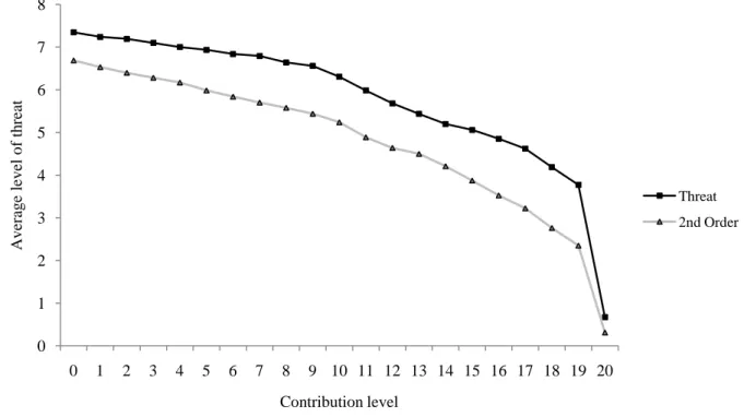
(10) can punish for the same motives as in the Threat treatment, but also on the basis of the difference between threatened and actual punishment assigned or received. In all treatments, the subgame perfect equilibrium is to not contribute at all to the public good and not to punish at any decision node. The marginal per capita return of the public good is always lower than the marginal return of keeping one‟s own endowment for oneself. In contrast, the socially optimal behavior is to contribute the full endowment of the public good, since 0.4*n > 1. In the treatments with threats, any profile of threats is compatible with the equilibrium since threats are cheap talk. No punishment is observed in equilibrium in any treatment since assigning punishment always reduces the payoff of the punisher. [Table 1 about here] 3. RESULTS This section is organized as follows. In section 3.1, we consider patterns in the assignment of threats. We then turn to the relationship between threats assigned and subsequent punishment. Then we consider the extent to which threats that are not followed through on draw sanctions. In section 3.2, we study the differences in contributions and earnings between treatments. The analysis in sections 3.1 and 3.2 concentrates on the HE condition. We focus on HE because it is a condition in which punishment is known to work, in the sense that typically induces a positive effect on contributions under Baseline conditions (Nikiforakis and Normann, 2009). In section 3.3, we consider whether the results are similar in the LE condition and establish that many of the patterns observed in HE are robust to the difference in punishment effectiveness. 3.1. Threats and sanctions 3.1.1. Assignment of threats Figure 1 displays the average threat assigned for each possible contribution level in each of the treatments in the High Effectiveness condition. The figure shows that threats are widely employed. In 83.75% of instances (469 observations out of 560), players make a. 7.

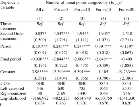
(11) threat in the Threat treatment. Threats are made in 87.36% of instances (629 observations out of 720) in the Second Order treatment. The figure also reveals that individuals make less severe threats for higher contributions, and for all possible contribution levels, the average threat is higher in the Threat than in the Second Order treatment. The average threat from one individual to another is 7.34 and 6.68 (this corresponds to an average threat to reduce earnings by approximately 70% of the non-cooperative equilibrium level) for a contribution level equal to zero in the Threat and Second Order treatments, respectively. On average, threats of 0.66 and 0.33 are made for the highest possible contribution of 20. In 11.61% of the observations in the Threat treatment, and 6.53% in the Second Order treatment, threat points are directed at even the highest possible contribution. Threats are on average considerably more severe for contributions just below the maximum, however. Averages of 3.77 and 2.34 threat points are assigned for a contribution of 19 in the Threat and Second Order treatments, respectively. 51.96% of the players in the Threat treatment, and 38.47% in the Second Order treatment, threaten to punish a contribution of 19. Our findings regarding threat decisions are summarized in Result 1. [Figure 1 and Table 2 about here] RESULT 1: Threats are widely employed, even against those making high potential contributions. Threats are more severe against lower contributions. For all contribution levels, threats are less severe in the Second Order treatment than in the Threat treatment. Threat severity increases over time, with the exception of the last period. Support for Result 1: Table 2 contains the estimates of five random-effects Tobit models, in which the dependent variable is the number of threat points that player i assigns to player j (for j≠i) for a given level of contribution c. In models (2) to (5), c takes the following values: c = 0, 10, 15, and 20. In all of the regressions, the independent variables include a dummy variable for the Second Order treatment (so that the Threat treatment is the reference category), a time trend, and a dummy variable for the final period.. 8.

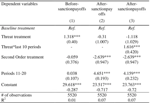
(12) The estimates show that significantly fewer threat points are assigned in the Second Order than in the Threat treatment for any positive contribution level except for c = 20. The significant time trend for all contribution levels except for the highest level of 20 indicates that threats tend to escalate over time. In another tobit regression (not reported here but available upon request), the dependent variable is the contribution threshold above which the player no longer threatens to punish. The independent variables are the same as in the regressions of Table 2. The results indicate that the contribution threshold, above which people cease threatening others, does not differ across treatments (coeff. = -0.497, S.E. = 1.165) and increases over time (coeff. = 0.085***, S.E. = 0.018) (N=3840, left censored observations=551, right-censored observations = 336; log-likelihood = -10331.63). 3.1.2. The relationship between threats and first order punishment We have seen that heavy threats are issued. We now consider the consistency of threats with subsequent punishment decisions. Our findings are reported in Result 2. RESULT 2. Actual sanctions are much less severe than those that are threatened. Threats are nevertheless positively correlated with subsequent sanctions. The severity of sanctions decreases over time, while the severity of threats increases over time. Support for Result 2: On average, subjects assign 0.423 punishment points in stage two of the Baseline treatment (S.D. = 1.42), 0.61 points in the Threat treatment (S.D. = 1.76), and 0.45 in the Second Order treatment (S.D. = 1.48). Mann-Whitney pairwise tests, with each group‟s decision as an observation, conclude that there is no difference in punishment levels between the Threat and the Baseline treatments (z =-0.380, p> 0.1), between the Second Order and the Baseline treatments (z =-0.795, p> 0.1), or between the Second Order and the Threat treatments (z = 0.476, p> 0.1). Figure 2 displays the average number of threat points and the actual number of punishment points assigned in the second stage of both the Threat and the Second Order treatments. These are displayed as a function of the difference between the target‟s contribution and the average group contribution (excluding j‟s contribution), in the High. 9.

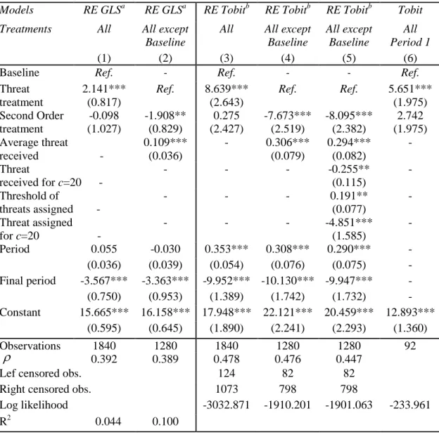
(13) Effectiveness condition. Figure 2 shows that punishers react strongly to negative deviations from the average contribution. For the purpose of comparison, the threat points are also shown in the figure. The figure suggests that the intensity of the threat level appears is a good indicator of subsequent punishment decisions, in the sense that threats and punishment are correlated. However, actual sanctions administered are far less severe than those that were threatened. For example, a subject who contributes between 15 and 20 units less than the group average in the Threat treatment receives on average 8.03 threat points but 3.92 punishment points. [Figure 2 about here] The left panel of Table 3 reports the estimates of three random-effects tobit models. The dependent variable is the number of punishment points that i assigns to j in the first punishment stage of period t. The first two models use the pooled data from the three treatments, while the third model uses the pooled data from the Threat and Second Order treatments. The independent variables include dummy variables for the treatment in effect, the average amount contributed by the group (excluding j‟s contribution), the differences between j‟s and the average contribution in the group conditional on j contributing less or more than the group average, a time trend, and a dummy variable for the final period. In the third model, the regressors also include the threat assigned by i for j‟s actual contribution. In addition, a dummy variable entitled “Anti-Social Threatener‟ indicates whether i has made a threat for the highest possible contribution. [Table 3 about here] Table 3 indicates that subjects receive more punishment, the less they have contributed relative to their group‟s average. This pattern is in agreement with previous studies (Fehr and Gächter, 2000; Masclet et al., 2003). Model (2) shows that, controlling for the differences between the target‟s and the average contribution in the group, subjects punish slightly more in the Threat treatment than in the Baseline. Estimated equation (3) in Table 3 shows that the stronger the prior threat, the more punishment points assigned. Furthermore, the subjects who threaten to punish the highest contribution. 10.

(14) level are more willing to sanction others. Thus, the severity of a threat is an indicator, albeit a biased one, of subsequent sanctioning decisions. 3.1.3. Threats and second order punishment In the Second-Order treatment, players may observe and punish differences between threatened and actual stage two sanctions. As we indicate in result three, empty threats, those that exceed the eventual punishment applied, are indeed sanctioned. RESULT 3.Individuals sanction those who fail to carry out their threats. Support for Result 3. Consider the three regressions reported in the right panel of Table 3. The dependent variable is the number of punishment points that i assigns to player j in the second round of sanctions in period t. In model (4), the independent variables are the average group contribution (excluding j‟s contribution) and the absolute values of positive, as well as of negative, differences between j‟s contribution and the average contribution of others.. The specification also includes, as dependent variables, the. average threat made by j to players k other than i for their actual contribution levels, and the number of punishment points j actually assigned to them. One dummy variable captures the impact of player j punishing less than he threatened, and another dummy indicates whether player i has been punished or not in the first round of sanctions. Model (5) includes the same variables as model (4) plus the positive and negative differences between the number of punishment points assigned by j to other players (excluding i) and the average assignment to these players. The positive and negative differences are written as:.       k1t max  p k1t  p / 2,0    j m    m j k i, j   k i    and.       max 0,    pmk1t  / 2   p k1t j   k i     m j k i, j . 11.

(15) respectively. Model (6) also includes a dummy variable indicating whether i has threatened the highest possible contribution of 20. The inclusion of this variable is intended to test whether anti-social threats are punished. The three estimations show that a subject is more likely to be punished in the second round of punishment, the fewer punishment points he assigned compared to the quantity he threatened to assign. We also find that empty threats are punished. However, there is also evidence of other motives to punish in this second punishment stage. Low contributions are punished again in this stage, as indicated by the significant coefficient associated with the negative difference between j‟s contribution and the group average. Moreover, a subject who has been punished in the first punishment stage is more likely to punish in the second punishment stage, even though he does not know who directed the punishment at him previously. The significant coefficient of the number of punishment points assigned by player j may indicate an attempt to counterpunish on the part of i, who might interpret a large assignment of punishment to others as an indication that j is likely to have been the one who punished i. Lastly, those who make anti-social threats are more likely to punish in the final punishment stage.6 3.1.4. Implications of receiving second order punishment on subsequent threats If failure to carry out threats is punished, subjects may react by reducing their threats. We observe that this is indeed the case, as argued in Result 4. RESULT 4.Threat behavior responds to the punishment of empty threats. In the Second Order treatment, subjects who punish less then they threaten to, and who are subsequently punished, decrease their threats in the next period. Support for Result 4. We have estimated a model of the determinants of changes in the threats made between periods t and t+1 (estimation available upon request). This model is estimated separately for the subjects who threatened more and those who threatened less than they actually punished in period t. The independent variables consist of both the 6. In an additional regression (available upon request), we have tested whether players punish those who engage in anti-social punishment in the first punishment stage. The coefficient of this variable is not significant, indicating that in our setting, second order punishment is not used to reciprocate or to deter anti-social punishment.. 12.

(16) difference between the number of threat points and the actual sanctions assigned by player i to his group members after being informed of their contribution levels, and the total number of punishment points received by i in the final stage of period t. The individuals who assigned more threat points than first-round punishment points in period t respond to second-round sanctions by revising downward the number of threat points they assign in the following period (coeff. = -0.170, p = 0.028).. Moreover, the. greater the difference in period t, the more they revise downward (coeff. = -0.452, p< 0.001). No such adjustment is observed for those who punished either equally or more severely than their threats (p = 0.570 and p = 0.814, respectively). 3.2. Contributions and earnings 3.2.1. The effect of threats and sanctions on contributions We now turn to treatment differences in contribution levels to examine whether threats influence cooperation. Figure 3 displays the time path of individual contributions by period, averaged across groups, in the three treatments, under the High Effectiveness condition. Our observations regarding contribution levels are described as Result 5. [Figure 3 about here] RESULT 5: The possibility of issuing threats increases cooperation. In the Threat treatment, average contributions are greater than in Baseline. However, permitting sanctions of differences between threatened and actual sanctions in the Second Order treatment reduces cooperation to a level equal to that in the Baseline treatment. Support for Result 5: As shown in Figure 3, non-binding threats of punishment increase average contributions in the High Effectiveness condition. The average contribution levels are highest in the Threat treatment (mean = 18.19 ECU per individual, S.D. = 3.32), followed by the Baseline (16.05 ECU, S.D. = 5.00), and by the Second Order treatment (15.95 ECU, S.D. = 4.90). Two-tailed Mann-Whitney pairwise tests, with each group average contribution over the session as an independent observation, indicate that the difference between the Baseline and Threat treatments (p = 0.06), as well as the difference between the Threat and the Second Order treatments (p = 0.08), are significant.. 13.

(17) In contrast, there is no significant difference between the Baseline and the Second Order treatments (p> 0.010). We have estimated several regressions in which the dependent variable is the player‟s contribution. Table 4 reports the results of these estimations. The independent variables include dummy variables for treatment, a time trend, and a dummy variable for the final period. When the data from all the treatments are pooled together (regressions 1, 3, and 6), the reference category is the Baseline. The independent variables also include the number of threat points received from the three other group members averaged over all possible contribution levels, and the total number of threat points received for the highest possible contribution of 20. They also include the threshold at which the subject no longer makes threats, and a dummy variable indicating whether the subject threatens others for the highest possible contribution. [Table 4 about here] Table 4 shows that the subjects contribute more in the Threat treatment than in the Baseline (see (1) and (3)). On average individuals invest 2.14 ECU more in the group account in the Threat treatment (regression (1)). Interestingly, participating in the Threat treatment makes a significant positive difference on contributions from the very beginning of the game, as indicated by regression (6). In contrast, controlling for the threats received, individuals contribute significantly less (-1.91 ECU) in the Second Order treatment than in the Threat treatment (regression (2)). The estimation of the tobit models confirms these findings. Models (2) and (4) also show that observing other players‟ threats increases cooperation significantly. In contrast, controlling for the general impact of threats, model (5) reveals that subjects react to anti-social threats (those directed towards the highest possible contribution) by reducing their contribution. This may be due to the expectation both of receiving sanctions for making a high contribution and of low cooperation on the part of the threatener. The higher is the threshold beyond which subjects no longer threaten, the more they cooperate. Those who assign threats for the highest possible. 14.

(18) contribution of 20 ECU cooperate significantly less. Contributions increase significantly over time (except in the final period). The number of sanctions received in the previous period has not been included in these regressions to avoid autocorrelation. To measure their impact, we have estimated the magnitude of some influences on changes in individual contributions between periods t and t+1 in separate random-effects GLS regressions (not reported here but available upon request). We conducted the estimations separately for the subjects who contribute less than the group average (designated as low contributors), and for those who contribute more than the average (high contributors), in period t (N = 457 and 1291, resp.; R2 = 0.429 and 0.081, resp.). We also included terms for interactions between the punishment received and treatment, as well as the difference between i‟s own and the others' average contributions. The estimates show that, while sanctions increase subsequent contributions of low contributors (coeff. = 0.316, p = 0.001), they have no impact on the behavior of high contributors (p = 0.635).. The impact of the first round of punishment on subsequent. contributions is similar in the Threat and the Second Order treatments as in Baseline (p = 0.763 and p = 0.487 for low contributors, p = 0.881 and p= 0.374 for high contributors, respectively). Similar regressions for the second round of punishment in the Second Order treatment indicate that sanctions received in the final punishment stage have no impact on subsequent contributions (low contributors: p = 0.178, N = 198, R2 = 0.546; high contributors: p = 0.191, N=284, R2 = 0.105), suggesting that receiving such sanctions is not interpreted as a punishment for a low contribution. 3.2.2. The effect of threats and sanctions on earnings As suggested earlier, if threats are effective in inducing greater cooperation, then the sanctions may not need to actually be implemented. Such a pattern would minimize the detrimental effects of punishment on efficiency and result in an improvement in overall welfare compared to a setting in which no threats can be sent. The data supports this hypothesis, but only partially, as summarized in Result 6.. 15.

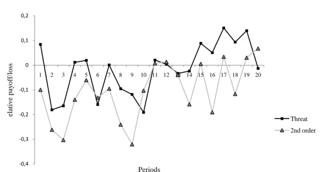
(19) RESULT 6. Threats increase earnings in the latter periods of the Threat treatment. However, the ability to punish discrepancies between threats and sanctions in the Second Order treatment, decreases welfare. Welfare in the Second Order treatment is below the Baseline treatment. Support for Result 6. The mean payoff after the contribution stage amounts to 29.63 ECU in the Baseline treatment (S.D. = 4.95), 30.92 in the Threat treatment (S.D. = 3.45), and 29.57 ECU in the Second Order treatment (S.D. = 5.20). However, the positive effect of threats on cooperation is partly offset by the cost of sanctions. The direct cost of punishment can be easily measured by comparing the average payoff after stage one and at the end of the period, in each treatment. The final payoffs amount to 25.84 ECU in the Baseline (S.D. = 8.31; this corresponds to 87.21% of the stage one payoff), 25.47 ECU in the Threat treatment (S.D. = 9.31; 82.37% of the stage one payoff), and 23.20 ECU in the Second Order treatment (S.D. = 11.17; 78.46% of stage one payoff). The relatively low payoff in the Second Order treatment results both from a smaller impact of threats on contributions, as well as from higher costs of punishment, due to the existence of two punishment stages. Figure 4 displays the differences in the average group payoff between the Threat and the Second Order treatments over time, normalized by subtracting the average group payoff of the Baseline treatment in the same periods. It illustrates the evolution of the relative payoff gain/loss in the Threat and Second Order treatments over time, respectively. Figure 4 shows that the Threat treatment succeeds in generating greater earnings than the Baseline treatment in the late periods. In contrast, the Second Order treatment induces a relative loss compared to the Baseline treatment throughout the session. Table 5 reports the estimations of three models, in which the dependent variable is the stage one payoff (model (1)), or the end of period payoff (models (2) and (3)). The independent variables include treatment, a time trend, and a dummy variable for the last 10 periods of a session. Lastly, a dummy variable interacting the Threat treatment and the last ten periods is also included in the estimates.. 16.

(20) [Table 5 and Figure 4 about here] The dummy variable for the last 10 periods is not significant in model (1) whereas it is positive and significant in models (2) and (3). This confirms the fact that final payoffs are significantly higher in the second half of the game as fewer sanctions are assigned over time. The Threat treatment induces significantly higher stage one payoffs than the Baseline (model (1)). A positive effect on welfare is also observed in terms of end-ofperiod payoffs in the second half of the game (model (3)). In contrast, in the Second Order treatment, payoffs do not differ from the Baseline after stage one, but are significantly lower at the end of the period. 3.3. The impact of punishment effectiveness In this subsection, we consider the data from the Low Effectiveness condition. As under HE, in the LE condition the average individual contributions are the highest in the Threat treatment (11.51, S.D. = 2.13), followed by the Baseline treatment (10.07, S.D. = 6.08), and by the Second Order treatment (8.86, S.D. = 5.39). Figure 5 displays the behavior of contributions over time. It shows that the effect of threats on contributions is less persistent over time than in the HE condition. Our findings are summarized in Result 7. [Figure 5 about here] RESULT 7: The severity of threats assigned is similar in the LE and the HE conditions. Under LE as under HE, the Threat treatment has a positive effect on the average contributions compared to the Baseline treatment. This effect is less persistent over time in the LE condition than in HE. Threats do not increase payoffs in this condition. Earnings are lower in the LE than in the HE condition. Support for Result 7: GLS regressions indicate that the contribution threshold at which a subject no longer assigns threat points is similar in the LE and HE conditions of the Threat treatment (N = 1280; p = 0.651) and of the Second Order treatment (N = 1440; p = 0.274). The same conclusion holds for every level of contribution in both treatments (p> 0.100), except that threats against the maximum contribution are higher in the LE than in the HE condition of the Second Order treatment (N =1440; p = 0.037).. 17.

(21) A Mann-Whitney pairwise test comparing average contributions in the Threat and the Baseline treatments in the LE condition indicates that people contribute significantly more in the Threat treatment than in the Baseline in the first ten periods (p=0.070). No significant difference is found between these treatments after period 10. While the average contribution is higher in the Threat than in the Second Order treatment in the first ten periods (p = 0.050), no significant difference is found in the second half of the game. A Mann-Whitney test comparing contributions in the Baseline treatment in HE (averaging 16.05 ECU) and in LE (averaging 10.07 ECU) indicates that people contribute significantly more in the HE condition (p = 0.007). Similar results are obtained when comparing contributions in the Threat treatment in the LE condition (11.51 ECU) and the HE condition (18.19 ECU) (p= 0.053), and when comparing contributions in the Second Order treatment in the LE (8.86 ECU) and HE conditions (15.95 ECU) (p= 0.012). There is no difference in final period earnings between the Baseline treatment (22.42) and the Threat treatment (22.97, p = 0.965), while payoffs are significantly lower in the Second Order treatment than in both the Baseline (16.29; p = 0.015) and the Threat treatments (p = 0.024). Final earnings are lower in LE than in HE for the Baseline (22.42 and 25.84 ECU; p = 0.101) and the Second Order treatment (16.29 and 23.20 ECU; p = 0.038). In the Threat treatment earnings are also smaller in the LE condition, but not significantly so (22.97 and 25.47 ECU; p = 0.315). 4. CONCLUSION Threats are common in human interaction and exchanges of threats often precede punishment. We have designed an experiment to study the effects of threats in a social dilemma setting in which the effect of punishment opportunities is well understood, the Voluntary Contributions Mechanism. The Baseline treatment is a classical VCM game with sanctions. The Threat treatment includes a preliminary stage in which subjects can assign non-binding threats to punish, as a function of potential contribution levels of other agents. The Second Order treatment augments the Threat treatment with an. 18.

(22) opportunity to observe and punish the differences between threats issued and actual punishment applied. We find that the ability to issue threats is welfare improving in the long run. It appears that to some extent, threats are believed, and cooperation can be increased with the punishment being carried out. However, the positive effect is negated if others cant monitor whether the threats made are actually carried out, and sanction those who fail to carry out their threats. When the latter is possible, threats are deterred, and fewer threats are used. The reduced level of threat, in turn, lowers contributions, and therefore overall welfare, returning then to levels even below those that would prevail in the absence of threats. Threats are widely used. Most individuals threaten up to a high level of contribution, although less severely in the Second Order than in the Threat treatment. It appears that threats to punish high contributions are at least to some extent due to the fact that people use threats in an attempt to coordinate on a certain level of contribution, and not only to signal their willingness to punish behavior of which they disapprove. While sanctions are much less severe than those that are threatened, the threats are nevertheless correlated with subsequent sanctions. In the Second Order treatment, individuals do sanction those who fail to carry out their threats, and players moderate their threats as a result. Threats increase the average contribution level, while the possibility of punishing differences between individual threats and actual sanctions hurts cooperation. We find no evidence that threats crowd out the intrinsic motivation to cooperate. Since the beneficial effect of threats on welfare develops only after a certain number of periods of interaction, it also suggests that threats might not be effective in short-run relationships. When a discrepancy between threatening and sanctioning behaviors is observable by the individuals, the effectiveness of threats vanishes completely. These results suggest that the use of threats is better suited to long-term interactions. In such a relationship, if threats and punishment can be associated, threats will only be effective if threateners are willing to follow through sufficiently often.. 19.

(23) REFERENCES. Anderson, C.M. and L. Putterman. 2006. "Do Non-Strategic Sanctions Obey the Law of Demand? The Demand for Punishment in the Voluntary Contribution Mechanism," Games and Economic Behavior, 54 (1), 1-24. Andreoni, J. 1988. “Why Free Ride: Strategies and Learning in Public Goods Experiments,” Journal of Public Economics, 35 (1), 57-73. Bochet, O., T. Page, and L. Putterman. 2006. “Communication and Punishment in Voluntary Contribution Experiments,” Journal of Economic Behavior and Organization, 60 (1), 11-26. Bochet, O., and L. Putterman. 2009. “Not just babble: Opening the black box of communication in a voluntary contribution experiment,”European Economic Review, 53 (3), 309-326. Brosig, J., A. Ockenfels,and J. Weimann, 2003. “The effect of communication media on cooperation,” German Economic Review, 4, 217–242. Carpenter, J.P. 2007a. “Punishing Free Riders: How Group Size Affects Mutual Monitoring and the Provision of Public Goods,” Games and Economic Behavior, 60 (1), 31-51. _______ 2007b.“The demand for punishment,”Journal of Economic Behavior and Organization, 62, 522–542. Cinyabuguma, M., T. Page, and L. Putterman. 2006. “Can Second Order Punishment Deter Perverse Punishment?,”Experimental Economics, 9 (3), 265-279. Denant-Boemont, L., D. Masclet and C. Noussair. 2007. “Punishment, Counterpunishment and Sanction Enforcement in a Social Dilemma Experiment,” Economic Theory, 31 (1), 145-167. Dickinson, D., and M.C. Villeval. 2008. “Does Monitoring Decrease Work Effort? The Complementarity Between Agency and Crowding-Out Theories,” Games and Economic Behavior, 63 (1), 56-76. Duffy, J., and N. Feltovich. 2006. “Words, deeds, and lies: strategic behaviour in games with multiple signals ,” The Review of Economic Studies 73 (3), 669-688. Egas, M. and A. Riedl. 2008. “The economics of altruistic punishment and the maintenance of cooperation,”Proceedings of the Royal Society B - Biological Sciences, 275 (1637), 871-878. Fehr E., and S. Gächter 2000. “Cooperation and Punishment in Public Goods Experiments,”American Economic Review, 90 (4), 980-94. Fehr, E., and B. Rockenbach. 2003. “Detrimental Effects of Sanctions on Human Altruism,” Nature, 422, 137-40. Fischbacher, U. 2007. “Z-Tree: Zurich Toolbox for Ready-made Economic experiments,”Experimental Economics, 10 (2), 171-178.. 20.

(24) Gächter, S., E. Renner, and M.Sefton. 2008. “The Long-Run Benefits of Punishment,”Science, 322, 5 December, 1510. Houser, D.,E. Xiao, K. McCabe, and V. Smith.2007. “Money, religion and revolution,” Economics of Governance, 8 (1), 1-16. _______. 2008.“When Punishment Fails: Research on Sanctions, Intentions and NonCooperation,”Games and Economic Behavior, 62 (2), 509-532. Isaac, R. M., K. McCue, and C. Plott. 1985. “Public Goods Provision in an Experimental Environment,” Journal of Public Economics, 26 (1), 51–74. Isaac, R. M., and J.M. Walker. 1988a. “Group Size Effects in Public Goods Provision: The Voluntary Contributions Mechanism,” Quarterly Journal of Economics, 103 (1), 179-99. _______. 1988b. “Communication and Free-Riding Behavior: The Voluntary Contributions Mechanism,” Economic Inquiry, 26 (4), 585-608. _______. 1991. “Costly Communication: An Experiment in a Nested Public Goods Problem," in T. Palfrey (Ed.). Contemporary Laboratory Research in Political Economy. Ann Arbor: Univ. of Michigan Press. Kerr, N.L., and C.M. Kaufman-Gilliland. 1994. “Communication, commitment, and cooperation in social dilemmas,” Journal of Personality and Social Psychology, 66, 513-529. Krishnamurthy, S. 2001. “Communication Effects In Public Good Games With And Without Provision Points,” in M. Isaac (Ed.). Research In Experimental Economics, Volume Eight, Amsterdam : JAI. Ledyard J. 1995. “Public Goods: A Survey of Experimental Research”, in Kagel J. and Roth. A., Eds., Handbook of Experimental Economics. Princeton: Princeton University Press, 111-194. Li, J., E. Xiao, D. Houser, and P.R. Montague. 2009. “Neural responses to sanction threats in two-party economic exchange,” PNAS, 106(39), 29 September, 1683516840. Marwell, G., and R.E. Ames. 1979. “Experiments on the provision of public goods. I: Resources, interest, group size, and the free-rider problem,” American Journal of Sociology, 84 (6), 1335–1360. Masclet, D., C. Noussair, S. Tucker and M.C Villeval. 2003. “Monetary and NonMonetary Punishment in the Voluntary Contributions Mechanism,” American Economic Review, 93 (1), 366-380. Nikiforakis, N. 2008.“Punishment and Counter-Punishment in Public Good Games: Can We Really Govern Ourselves?,” Journal of Public Economics, 92, 91–112. Nikiforakis, N. and H. Normann. 2008. “A Comparative Statics Analysis of Punishment in Public Goods Experiments”, Experimental Economics, 11, 358-369.. 21.

(25) Noussair, C., and S. Tucker. 2005. “Combining Monetary and Social Sanctions to Promote Cooperation,” Economic Inquiry, 43 (3), 649-660. Ostrom, E., J. Walker, and R. Gardner. 1992. “Covenants With and Without a Sword: Self-Governance Is Possible,”American Political Science Review, 86 (2), 404–417. Sefton, M., R. Shupp, and J. Walker, 2007. “The Effect of Rewards and Sanctions in Provision of Public Goods,” Economic Inquiry, 45, 671-690. Yamagishi, T. 1986. “The Provision of a Sanctioning System as a Public Good,” Journal of Personality and Social Psychology, 51 (1), 110-116.. 22.

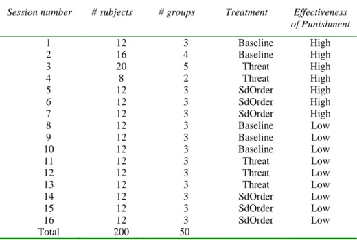
(26) Table 1. Characteristics of the experimental sessions Session number 1 2 3 4 5 6 7 8 9 10 11 12 13 14 15 16 Total. # subjects 12 16 20 8 12 12 12 12 12 12 12 12 12 12 12 12 200. # groups 3 4 5 2 3 3 3 3 3 3 3 3 3 3 3 3 50. 23. Treatment Baseline Baseline Threat Threat SdOrder SdOrder SdOrder Baseline Baseline Baseline Threat Threat Threat SdOrder SdOrder SdOrder. Effectiveness of Punishment High High High High High High High Low Low Low Low Low Low Low Low Low.

(27) Table 2. Determinants of threat assignment: High Effectiveness condition (randomeffects Tobit models) Dependent variable. Threat treatment Second Order treatment Period Final period. Number of threat points assigned by i to j, j≠ All c. For c=0. For c=10. For c=15. For c=20. (1) Ref.. (2) Ref.. (3) Ref.. (4) Ref.. (5) Ref.. -0.837*. -4.547***. -1.944*. -1.905*. -2.510. (0.509). (1.791). (1.111). (1.021). (2.211). 0.130***. 0.245***. 0.244***. 0.391***. -0.119*. (0.007). (0.027). (0.018). (0.018). (0.067). -0.930*** -2.844*** -2.006*** -2.649*** (0.195). (0.722). (0.475). -0.409. (0.459). (1.883). 1.185. -19.733***. Constant. 3.983*** 12.399*** 5.591***. # Obs. Left-censored Right-censored Log-likelihood . (0.391) (1.404) (0.856) (0.790) 3840 3840 3840 3840 546 630 735 1065 30 2169 1440 1068 -8166.982 -4823.275 -6514.949 -6650.759 0.684 0.763 0.701 0.670. (2.180) 3840 3504 246 -1541.330 0.620. Notes: *** Significant at the 0.01 level; ** at the 0.05 level; * at the 0.1 level. The “Threat treatment” variable is omitted as it is the reference category. The “Second Order treatment” variable is a dummy that equals 1 if the subject plays the Second Order treatment, and 0 otherwise. The “Period” variable is a time trend. “Final Period” is a dummy that equals 1 if the current period is the last one, and 0 otherwise.. 24.

(28) Table 3. Determinants of the number of punishment points assigned by player i to player j in the two rounds of punishment: High Effectiveness condition (random-effects Tobit estimates) Treatments. Baseline treatment Threat treatment Second Order treat. Average contribution of other group members (c-i) Absolute pos. diff. from group average contrib. Absolute neg. diff. from group average contrib. Threat i assigned to j. (1) Ref. 0.378 (0.702) 0.488 (0.657) -. First round of punishment All All except treatments Baseline (2) (3) Ref. 1.212* Ref. (0.670) 0.383 -0.893 (0.624) (0.582) -0.221*** -0.160*** (0.033) (0.044) -0.297*** -0.236*** (0.051) (0.063) 0.525*** 0.407*** (0.021) (0.027) 0.377*** (0.042) 1.364*** (0.380) -. Second round of punishment Second Order treatment (4) -. (5) -. (6) -. -. -. -. 0.112** (0.055) 0.001 (0.069) 0.283*** (0.028) -. 0.112** (0.057) 0.001 (0.069) 0.283*** (0.028) -. 0.117** (0.056) -0.003 (0.069) 0.282*** (0.028) -. -. -0.033 (0.081) 0.498** (0.227) 0.769* (0.428) 1.393*** (0.349) 0.012 (0.250) 0.023 (0.127) -0.171*** (0.030) -0.073 (0.933) -6.875*** (1.150) 2160 1892 -1069.911 0.375. 0.906* (0.490) -0.028 (0.081) 0.502** (0.225) 0.702* (0.427) 1.356*** (0.346) 0.007 (0.249) 0.028 (0.127) -0.160*** (0.030) -0.092 (0.924) -7.024*** (1.139) 2160 1892 -1068.230 0.355. i is Anti-social threatener. -. j's average threat. -. j's average punishment in first round j threatens more than he punishes Sanctions i received in first round Pos. diff. between j’s and average first round punishment Neg. difference between j’s and Average first round punishment Period. -. -. -. -. -. -. -. -. -. -. -. -. -0.033 (0.081) 0.502*** (0.098) 0.777* (0.425) 1.390*** (0.345) -. -. -. -. -. -0.329*** (0.023) -0.455 (0.695) -0.224 (0.923) 3840 565 30 -2204.581 0.486. -0.171*** (0.029) -0.072 (0.933) -6.866*** (1.119) 2160 1892 -1069.927 0.375. Final period dummy Constant # observations # left cens.obs. # right cens.obs. Log-likelihood . -. -0.314*** (0.019) 0.100 (0.567) -6.902*** -0.051*** (0.549) (0.728) 5520 5520 4676 4676 46 46 -3802.420 - 3212.445 0.373 0.521. Notes :*** Significant at the 0.01 level; ** at the 0.05 level; * at the 0.1 level. Standard errors are in parentheses. The “Baseline treatment” variable is omitted as it is the reference category. The “Threat (Second Order, respectively) treatment” variable is a dummy that takes 1 if the subject plays the Threat (Second Order, respectively) treatment, and 0 otherwise. The “Threat i assigned to j” variable is the number of threat points assigned by i for a level of contribution equal to that of player j. The “Anti-social punisher” variable takes value 1 if i assigned threat points for the highest possible contribution level, and 0 otherwise. The “j's average threat” variable indicates the average number of threat points assigned by j for each possible contribution level. The “j's average punishment in first round” variable captures the average number of punishment points assigned by j to the players other than i. The “j threatens more than he punishes” variable is a dummy equal to 1 if j has assigned more punishment points than threat points, and 0 otherwise. The “Received sanctions in first round” variable is the total number of points i has been assigned by the other players. The “Positive deviation of j from average punishment in first round” variable is equal to 1 if j has punished more than the other players, and 0 otherwise. The “Negative deviation of j from average punishment in first round” variable is equal to 1 if j has. 25.

(29) punished less than the other players, and 0 otherwise. The “Period” variable is a time trend. The “Final period” variable is equal to 1 if the observation corresponds to the final period of the game, and 0 otherwise.. 26.

(30) Table 4. Determinants of contributions in the High Effectiveness condition Models Treatments. RE GLSa. RE GLSa. RE Tobitb. RE Tobitb. RE Tobitb. Tobit. All. All except Baseline (2) Ref.. All. All except Baseline (4) Ref.. All except Baseline (5) Ref.. All Period 1 (6) Ref. 5.651*** (1.975) 2.742 (1.975) -. (1) Baseline Ref. Threat 2.141*** treatment (0.817) Second Order -0.098 treatment (1.027) Average threat received Threat received for c=20 Threshold of threats assigned Threat assigned for c=20 Period 0.055 (0.036) Final period -3.567*** (0.750) Constant 15.665*** (0.595) Observations. . 1840 0.392. Lef censored obs. Right censored obs. Log likelihood R2 0.044 Notes:. -1.908** (0.829) 0.109*** (0.036) -. (3) Ref. 8.639*** (2.643) 0.275 (2.427) -. -8.095*** (2.382) 0.294*** (0.082) -0.255** (0.115) 0.191** (0.077) -4.851*** (1.585) -0.030 0.353*** 0.308*** 0.290*** (0.039) (0.054) (0.076) (0.075) -3.363*** -9.952*** -10.130*** -9.947*** (0.953) (1.389) (1.742) (1.732) 16.158*** 17.948*** 22.121*** 20.459*** (0.645) (1.890) (2.241) (2.293) 1280 0.389. 1840 0.478 124 1073 -3032.871. -7.673*** (2.519) 0.306*** (0.079) -. 1280 0.476 82 798 -1910.201. 1280 0.447 82 798 -1901.063. 12.893*** (1.360) 92. -233.961. 0.100. a. Random-effects Generalized Least Squares model with robust standard errors clustered at the b individual level in parentheses; random-effects tobit; *** significant at the 0.01 level; ** at the 0.05 level; * at the 0.1 level. The “Baseline treatment” variable is omitted as it is the reference category. The “Respect (Second Order, respectively) treatment” variable is a dummy that takes 1 if the subject plays the Respect (Second Order, respectively) treatment, and 0 otherwise. The “Average threat received” variable is the sum of threat points received by a subject from his three group members. The “Threat received for c=20” variable is the sum of threat points received by a subject from his three group members if his contribution is equal to 20. The “Threshold of threats assigned” is the contribution (between 0 and 20) from which a subject stops threatening others. The “Threat assigned for c=20” variable indicates the number of threat points assigned by the subject for a contribution equal to 20. The “Period” variable is a time trend. The “Final period” variable is equal to 1 if the observation corresponds to the final period of the game, and 0 otherwise.. 27.

(31) Table 5. Determinants of payoffs in the HE condition (random-effects GLS models) Dependent variables. Baseline treatment Threat treatment Threat*last 10 periods Second Order treatment. Periods 11-20 Constant # of observations R2. Beforesanctionpayoffs. Aftersanctionpay offs. Aftersanctionpayoffs. (1). (2). (3). Ref.. Ref.. Ref.. 1.318*** (0.40) -. -0.31 (1.007) -. -0.059 (0.376). -2.639*** (0.947). -1.118 (1.029) 1.616*** (0.420) -2.639*** (0.947). 0.038 (0.107) 29.618*** -0.287 5520 0.01. 4.651*** (0.193) 23.517*** -0.717 5520 0.07. 4.159*** (0.232) 23.763*** -0.72 5520 0.07. Note: *** significant at the 0.01 level; ** at the 0.05 level; * at the 0.1 level. Robust standard errors in parentheses with clustering at the individual level. The “Baseline treatment” variable is omitted as it is the reference category. The “Respect (Second Order, respectively) treatment” variable is a dummy that takes 1 if the subject plays the Respect (Second Order, respectively) treatment, and 0 otherwise. The “Period 11-20” variable is equal to 1 if the observation belongs to the second half of the experiment, and 0 otherwise.. 28.

(32) 8 7. Average level of threat. 6 5 4 Threat. 3. 2nd Order. 2 1 0 0. 1. 2. 3. 4. 5. 6. 7. 8. 9 10 11 12 13 14 15 16 17 18 19 20. Contribution level. Figure 1. Average number of threat points assigned for each contribution level by treatment in the High Effectiveness condition. 29.

(33) Average number of points of threat and sanction assigned. 9 27. 8 84. 7. 36. 66. Actual punishment Threat. 6. Announcement Threat. 5. Actual punishment 2nd Order. 27. 4 3. 105. 84. Announcement 2nd order. 171. 36 54. 66. 2. 105. 171. 1 0 [-20,-14). [-14,-8). [-8,-2). 444 1329 219 1263 219 1263 444 1329. [-2,2]. (2,8]. 30 30 54. (8,14]. (14,20]. Difference of contribution between j and the average of others. Figure 2. Average individual threat and actual punishment by treatment and by category of difference between j‟s and the average group contribution of others, in the High Effectiveness condition. 30.

(34) 20. Average individual contribution. 19 18 17 16 15. Baseline. 14. Threat. 13. 2nd Order. 12 11 10 1. 2. 3. 4. 5. 6. 7. 8. 9. 10 11 12 13 14 15 16 17 18 19 20. Periods. Figure 3. Average individual contributions over time by treatment in the High Effectiveness condition. 31.

(35) R 0,2. elative payoff/loss. 0,1. 0 1. 2. 3. 4. 5. 6. 7. 8. 9. 10 11 12 13 14 15 16 17 18 19 20. -0,1. -0,2. Threat 2nd order. -0,3. -0,4. Periods. Figure 4. Average payoff difference between threat and second order treatments relative to the Baseline treatment in the High Effectiveness condition. 32.

(36) 16. Average individual contribution. 14 12 10. Baseline. 8. Threat 2ndOrder. 6 4 2 0 1. 2. 3. 4. 5. 6. 7. 8. 9. 10 11 12 13 14 15 16 17 18 19 20 Periods. Figure 5. Average individual contributions over time by treatment in the Low Effectiveness condition. 33.

(37) Appendix. Instructions of the Threat treatment (high effectiveness condition)(Translated from the original French text. The instructions for the other treatments are available upon request) You are taking part in an economic experiment, during which you can earn money. Your earnings depend on your decisions and on the decisions of the other participants with whom you will interact. It is therefore important to read these instructions with attention. All of the transactions during the experiment and your entire earnings will be calculated in ECU (Experimental Currency Units). At the end of the experiment, the total amount of ECU you have earned during this session will be converted to Euros, and paid to you in cash in a separate room. You will be paid by somebody who is not aware of the content of the experiment, according to the following rules: . Your final payoff in ECU consists of the total of your payoffs in each of the 20 periods that make up this session. . This final payoff in ECU will be converted into Euros at the rate: 100 ECU = 2 Euros.. . In addition, you will be given a show up fee of 5 Euros.. At the beginning of the session, the participants are divided into groups of four. You will therefore interact with three other participants. During the 20 periods, you will interact with the same persons. You will never be informed of the identity of these persons. Description of each period In each period, after receiving an endowment of 20 ECU each, the four participants belonging to a group can participate in a project, by contributing to a group account that will be shared among them. The amount of this group account is determined by the total of the individual contributions of the four members of the group. Next, the group members can indicate their disapproval of the contribution of other members of the group by assigning points that reduce their payoff. Each period consists of three stages: -. During the first stage, each group member indicates how many disapproval points he would be ready to assign to other group members for each possible contribution level in the second stage.. -. During the second stage, after being informed of the number of disapproval points that the other group members propose to assign for each possible contribution level, each of the four group members decides simultaneously on his actual contribution to the project.. -. During the third stage, after being informed of the individual contributions of the other group members, each one decides on the number of disapproval points he actually assigns to other group members and their payoffs are reduced accordingly.. The details of each stage are described below. First stage You announce the number of points you would like to assign to each other group member for each possible contribution level (between 0 and 20 ECU)to the project in the second stage. The number of points you announce for a group member indicates your degree of disapproval for each contribution level (from 10 points for the highest disapproval to 0 point for no disapproval). The three other members of your group are informed of your announcement before they decide on their contribution level. For the moment, the points you announce affect neither your payoffs nor the payoffs of your group members. They simply indicate to the others your willingness to reduce their payoffs for each possible contribution amount. It is only after every group member will have decided his contribution during the. 34.

(38) second stage that you will, in the third stage, confirm or modify your announced number of points. These points will then affect both your payoffs and the payoff of your group members, as indicated below. . You announce the number of points that you would be willing to assign for each possible contribution level of the other members of your group. You must enter a number, between 0 and 10, for each possible contribution. If you do not want express disapproval, you must enter 0.. . At the end of the first stage, the number of points you would be willing to assign for each contribution level will be announced to the members of your group. You are also informed of the total number of points that your three group members are willing to assign to you in the third stage for each of your possible contribution levels.. Below is the screenshot for the first stage.. Second stage You receive an endowment of 20 ECU. After being informed of the total number of points that you are susceptible to receiving from the other group members for each possible contribution level, you decide on your contribution to the project.. 35.

(39) You, as well as the three group members decide simultaneously, how much of your endowment you will allocate to the project, by indicating a number between 0 and 20. To validate your choice, click the OK button. After all group members have made their decision, your screen will show you the total amount of ECU contributed to the project by the members of your group (including your contribution). You are also informed of your current payoff at this stage. Your payoff at this second stage consists of two parts:  the amount of your endowment which you have kept for yourself (that is, 20 – your contribution to the project),  your income from the project: this income represents 40% of the total contribution of all four group members to the project . Your payoff in ECU in this second stage is computed by the program as follows: (20-your contribution to the project) + 40%*(total contributions of the group to the project) Below is the screenshot for the second stage.. The payoff of each group member is calculated in the same way, which means that each group member receives the same income from the project.. 36.

(40) For example, suppose that the total of the contributions of all group members is 60 ECU. In this example each member of the group receives a second-stage payoff from the project of 40% (of 60 ECU) = 24 ECU. On the other hand, if the total contribution to the project is 9 ECU, then each member of the group receives 40% (of 9 ECU) = 3.6 ECU from the project. For each ECU of your endowment that you keep for yourself you earn an income of 1 ECU. Every ECU you contribute to the project instead increases the total contribution to the project by one ECU. The income from the project will increase by 0.4 ECU per person and so, the total income of the group from the project will rise by 1.6 ECU. This means that your contribution to the project also increases the income of the other group members. On the other hand you will earn money from each ECU contributed by the other members to the project. For each ECU contributed by any group member you earn 40% (1) = 0.4 ECU.. Third stage After being informed of the contribution of each of the other members of your group, you can, if you would like, reduce or leave unchanged their payoff by assigning points. This number of points can be the same or different from the number you have announced in the first stage.You can assign a particular number of points to a member of your group to express a level of disapproval (10 points for the highest disapproval, 0 points for no disapproval). Each point assigned to a particular group member reduces her second-stage income by two points. Your decision during the third stage depends on the actual contributions and can change both your payoff and the payoff of the other members of your group. Similarly, your payoff can be changed if the other group members wish to do so. . You are informed of the contribution of each of the other three members of your group to the project in the second stage of the game. Note: the order in which each contribution is displayed changes randomly in each period (in other words, for example, the number that appears first on your screen does not always correspond to the decision of the same player).. . You decide next on how many points to send to each of the other three members of your group to reduce their payoff or leave it unchanged. Each point assigned to a group member reduces his second-stage payoff by 2 ECU. If you assign 0 point to another member, you do not change hissecond-stage payoff. If you assign 1 point to a group member, you reduce his second-stage payoff by 2ECU; if you assign 2 points, you reduce his second-stage payoff by 4 ECU; etc. You must enter a value for each member, between 0 and 10 points. If you do not wish to reduce the payoff of a specific member, then you must enter 0.. . If you assign points, you pay a cost that depends on the number of points you assign to each subject. Each point you assign reduces your second-stage payoff by 1 ECU. Your total cost is equal to the sum of the costs of assigning points to each of the other three group members. If you assign two points to one group member, it will cost you 2 ECU. If you assign 9 points to another member, it will cost you 9 ECU more. If you give the last group member no points, it does not cost you anything. In this example, the total cost of the assigned points is 11 ECU (2+9+0). These costs will be displayed on your screen. You can modify your decisions until you click the OK button.. Below is the screenshot for the third stage.. 37.