Analyse spatiale des assemblages de mammifères marins de
l’estuaire du Saint-Laurent
Mémoire présenté dans le cadre du programme de maîtrise en océanographie en vue de l’obtention du grade de maître ès sciences
PAR
© CLAUDIE LACROIX-LEPAGE
Composition du jury :
Gesche Winkler, présidente du jury, Université du Québec à Rimouski Véronique Lesage, directrice de recherche, Institut Maurice-Lamontagne Philippe Archambault, codirecteur de recherche, Université Laval
Charlotte Moritz, membre externe, CMOANA Consulting
UNIVERSITÉ DU QUÉBEC À RIMOUSKI Service de la bibliothèque
Avertissement
La diffusion de ce mémoire ou de cette thèse se fait dans le respect des droits de son auteur, qui a signé le formulaire « Autorisation de reproduire et de diffuser un rapport, un
mémoire ou une thèse ». En signant ce formulaire, l’auteur concède à l’Université du
Québec à Rimouski une licence non exclusive d’utilisation et de publication de la totalité ou d’une partie importante de son travail de recherche pour des fins pédagogiques et non commerciales. Plus précisément, l’auteur autorise l’Université du Québec à Rimouski à reproduire, diffuser, prêter, distribuer ou vendre des copies de son travail de recherche à des fins non commerciales sur quelque support que ce soit, y compris l’Internet. Cette licence et cette autorisation n’entraînent pas une renonciation de la part de l’auteur à ses droits moraux ni à ses droits de propriété intellectuelle. Sauf entente contraire, l’auteur conserve la liberté de diffuser et de commercialiser ou non ce travail dont il possède un exemplaire.
Je dédie ce mémoire à ma famille qui a toujours cru en moi.
Rome ne s’est pas construite en criant : « Lapin, je ne boirai pas de ton eau ! » Capitaine Charles Patenaude
REMERCIEMENTS
Je tiens d’abord à remercier Véronique et Philippe de m’avoir supervisée et soutenue tout au long de ce projet au cours duquel j’ai eu la chance de participer à plusieurs formations, conférences et expériences de terrain qui m’ont fait grandir, tant au niveau professionnel que personnel. Je vous suis reconnaissante de m’avoir offert cette opportunité de travailler sur un sujet qui me passionne et qui continuera de me passionner longtemps. Je veux également remercier Arnaud Mosnier et Jean-François Gosselin, sans qui la réalisation de ce projet aurait été impossible. Merci à tous de votre aide et de votre temps.
Je souhaite ensuite remercier Gesche Winkler et Charlotte Moritz d’avoir accepté d’agir à titre de présidente du jury et de membre externe lors du dépôt initial de ce mémoire. J’aimerais remercier mes amis - de Rimouski, de Montréal et d’ailleurs - qui ont été un véritable système de soutien, dans les meilleurs moments comme dans les pires. Merci de votre soutien et de votre écoute. Un merci particulier à Marie, mon amie et collègue de labo. Sans toi, ces dernières années auraient été bien moins agréables.
Finalement, il est difficile d’imaginer à quoi aurait ressemblé mon parcours sans l’aide de ma famille. Doris, André et Marilou - vous avez été mon phare. Vous m’avez écoutée, vous m’avez encouragée, mais surtout, vous avez cru en moi, même quand moi je n’y croyais plus. Pour ces raisons, et pour tellement d’autres encore, je vous dois tout et vous remercie du fond du cœur. Papa - merci d’avoir passé toutes ces heures à relire mon texte. Maman - merci de m’avoir écoutée quand j’avais besoin de ventiler. Malou - merci de m’avoir fait rire pendant nos cafés Skype. Antho - merci pour tous nos beaux moments passés ensemble, et pour ceux à venir. Je vous aime.
RÉSUMÉ
Une des conditions essentielles de la préservation de la biodiversité des espèces est de comprendre les facteurs qui influencent leur distribution. L’importance de l’estuaire du Saint-Laurent (ESL) pour plusieurs espèces de mammifères marins de l’Atlantique Nord-Ouest est reconnue depuis longtemps, mais il existe très peu de données spatiales et temporelles sur leur abondance et leur distribution dans cette région. La modélisation prédictive peut aider à combler le manque d’information et à interpoler les prédictions de distribution sur l’aire potentielle d’utilisation par les mammifères marins. Un total de 4012 observations, portant sur neuf espèces de mammifères marins, recueillies lors de 100 relevés hebdomadaires effectués entre 2009 et 2014 dans l’estuaire maritime du Saint-Laurent, a servi à générer des cartes de probabilité de distribution des assemblages de mammifères marins sur l’ensemble de l’ESL. Une classification hiérarchique a été utilisée afin de définir les assemblages en regroupant les observations de mammifères marins en fonction de la similitude des relations entre les mammifères marins observés et quatre variables océanographiques, à savoir la température et la salinité de surface moyennes, la profondeur et la pente du fond. Les assemblages ont été caractérisés et leur biodiversité a été évaluée à l’aide d’indices écologiques. Le regroupement a révélé quatre assemblages utilisant trois types d’habitats : les eaux profondes du secteur du chenal Laurentien, les eaux peu profondes côtières et à la tête du chenal, et la pente du chenal. Les indices de diversité ont indiqué que les assemblages retrouvés dans les eaux peu profondes et la pente du chenal sont les plus diversifiés. Un modèle de régression logistique multinomiale a par la suite été utilisé afin de produire des cartes de distribution montrant la probabilité d’occurrence des assemblages en fonction des quatre variables océanographiques énumérées ci-dessus. Cet exercice a permis de qualifier l’importance des zones habituellement difficiles à qualifier en raison d’un manque de données. Ces nouvelles connaissances sur la biodiversité des mammifères marins de l’ESL pourraient aider à comprendre et prévoir les changements potentiels de la distribution des assemblages et de l’occurrence des espèces en réponse aux effets à long-terme des changements environnementaux, et ainsi contribuer à l’élaboration de mesures de conservation visant à protéger ces animaux.
Mots clés : mammifères marins, assemblages, estuaire du Saint-Laurent, modélisation prédictive, biodiversité
ABSTRACT
Understanding the distribution of species is a key prerequisite for the preservation of biodiversity. The St. Lawrence Estuary (SLE) has long been recognized as an important ecosystem for marine mammals of the western North Atlantic, but little data are available to assess the abundance and distribution of these species at different temporal and spatial scales. Predictive modeling can be used to fill these gaps and interpolate distribution predictions over the potential range of species. A total of 4,012 sightings of nine species detected during 100 weekly surveys carried out between 2009 and 2014 in the Lower SLE were used to generate probability distribution maps of marine mammal assemblages for the SLE as a whole. Hierarchical clustering was used to define assemblages by grouping marine mammal sightings according to the similarity of their relationships with mean sea surface temperature and salinity, depth and slope. The resulting assemblages were characterized, and their diversity was measured using diversity indices. Hierarchical clustering revealed four assemblages found in three types of habitats: deeper waters of the Laurentian Channel, shallower waters near the coast and at the head of the Channel, and slope of the Channel. Diversity indices indicated that assemblages found in shallower waters and on the slope of the Channel were more diverse. A multinomial logistic regression model was then used to generate distribution maps showing the probability of assemblage occurrence based on the four environmental variables. This exercise allowed us to qualify the importance of areas usually difficult to qualify due to the lack of data. This increased knowledge of marine mammal biodiversity in the SLE could help us understand and predict the potential changes in assemblage distribution and species occurrence in response to long-term climate change effects, and therefore has the potential to guide the development of efficient management actions for the conservation of these animals.
Keywords: marine mammals, assemblages, St. Lawrence Estuary, predictive modeling, biodiversity
TABLE DES MATIÈRES
REMERCIEMENTS ... ix
RÉSUMÉ ... xi
ABSTRACT ... xiii
TABLE DES MATIÈRES ... xv
LISTE DES TABLEAUX ... xvii
LISTE DES FIGURES ... xix
INTRODUCTION GÉNÉRALE ... 1
CHAPITRE 1 : SPATIAL ANALYSIS OF MARINE MAMMAL ASSEMBLAGES IN THE ST. LAWRENCE ESTUARY (CANADA) ... 11
1.1 INTRODUCTION ... 11
1.2 METHODOLOGY ... 16
1.2.1 Study area ... 16
1.2.2 Surveys and marine mammal sightings ... 17
1.2.3 Environmental data ... 19
1.2.4 Statistical analysis and modeling framework ... 22
1.3 RESULTS ... 27
1.3.1 Marine mammal sightings ... 27
1.3.2 Environmental correlates and marine mammal assemblages ... 33
1.3.3 Species composition and biodiversity of marine mammal assemblages ... 40
1.3.4 Predictive modeling of marine mammal assemblage distribution ... 43
1.4 DISCUSSION ... 54
1.4.2 Species composition of marine mammal assemblages ... 56
1.4.3 Biodiversity of marine mammal assemblages ... 62
1.4.4 Interpretation of model predictions in the context of climate change ... 63
1.4.5 Acknowledgments ... 66
CONCLUSION GÉNÉRALE ... 67
LISTE DES TABLEAUX
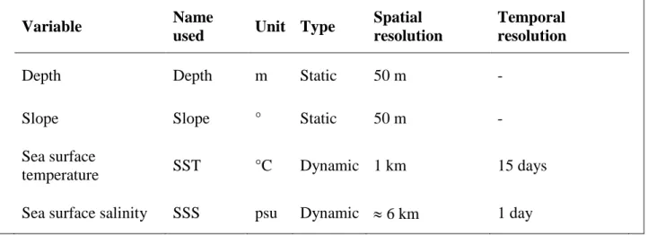
Table 1. Names, time periods and days used for the extraction of mean sea surface temperature over the 15 days previous to the sighting including survey date (SST15) and estimation of mean sea surface salinity on survey date (SSS1) for the five scenarios used to model assemblage membership for each 1 km cell of the prediction grid. ... 25 Table 2. Number of sightings and proportions (%) of sightings and individuals, mean group size and standard deviation (± SD) of encountered marine mammal species in the Lower St. Lawrence Estuary (LSLE). ... 32 Table 3. Pearson’s correlation coefficients (r) of environmental variables in the initial dataset. SST1, SST3, SST5, SST7 and SST15 stand for mean sea surface temperature over the 1, 3, 5, 7 and 15 days previous to the sighting including survey date. SSTc3 and SSTc5 stand for mean sea surface temperature averaged and centered on 3 and 5 d periods. SSTlag3, SSTlag5, SSTlag7 and SSTlag15 stand for mean sea surface temperature averaged and centered on a 3 d period with 3, 5, 7 and 15 d lags. SSS1 stands for mean sea surface salinity on survey date. ... 34 Table 4. Characteristics of the environmental variables selected for the analysis. ... 35 Table 5. Species richness, diversity and evenness for the four marine mammal assemblages within the Lower St. Lawrence Estuary (LSLE). ... 43 Table 6. Set of models explaining the occurrence of marine mammal assemblages. Variables included were mean sea surface temperature over the 15 days previous to the sighting including survey date (SST15), mean sea surface salinity on survey date (SSS1), depth and slope. Residual deviance is a measure of goodness of fit and AIC indicates the quality of models. For both measures, the highest number reflects the worst fit. ... 44 Table 7. Misclassification matrix. Columns represent the actual assemblage membership of marine mammal sightings. Lines represent the predictions of the model. Numbers on the diagonal represent the correct classification. ... 45
Table 8. Output of the multinomial logistic regression pertaining to the significance of environmental variables with the a) estimated coefficients, b) standard errors and c) Wald statistics. Assemblage 1 was used as the pivot category. Coefficients are relative to the pivot category and estimate the rate at which the log of the odd ratios of two assemblages changes as predictor variables change in ratio per unit. The generic equation of the MLR model is 𝑙𝑛(𝑃𝑟𝑜𝑏. 𝑌/𝑃𝑟𝑜𝑏. 1) = 𝛽0 + 𝛽1(𝑆𝑆𝑇15) + 𝛽2(𝑆𝑆𝑆1) + 𝛽3(𝐷𝑒𝑝𝑡ℎ) + 𝛽4(𝑆𝑙𝑜𝑝𝑒), where the response variable Y, i.e., the probability of sightings falling into a given assemblage in terms of the four environmental variables (X), are the log odds for all other assemblages (2, 3 or 4) relative to the pivot assemblage (1). Asterisks next to coefficients indicate significant estimated regression coefficients at P < 0.05. ... 46
LISTE DES FIGURES
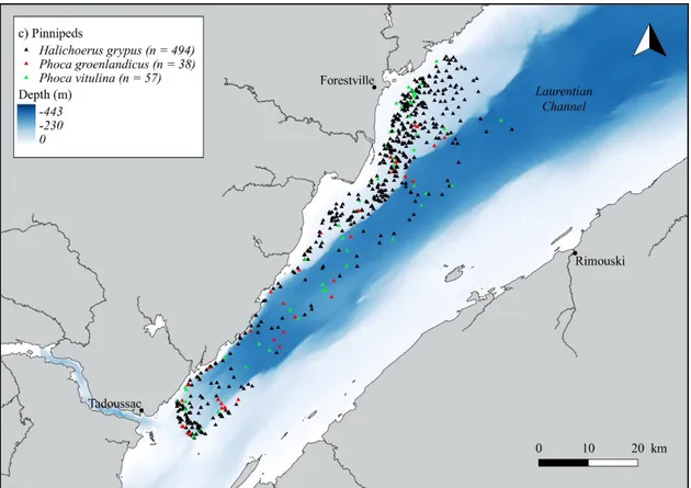
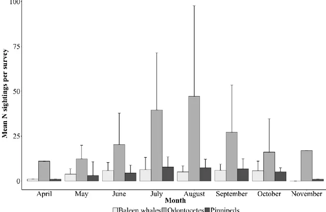
Figure 1. The Estuary and Gulf of St. Lawrence, Eastern Canada. The area where this study took place (in red) is located in the Lower St. Lawrence Estuary (LSLE). ... 17 Figure 2. Typical sampling design on a survey day in the Lower St. Lawrence Estuary (LSLE). The red line delineates the area in which surveys were done. The black line is an example of a track followed by the research vessel. Observers were on effort when surveying perpendicular to the coast; only opportunistic sightings were collected during transits between transects (parallel to the coast) and these were not included in the analysis. Depth data were obtained from a 50 m resolution raster created by interpolating data from the Canadian Hydrographic Service. ... 18 Figure 3. Bottom slope (in degrees) of the Lower St. Lawrence Estuary (LSLE) computed from depth data obtained from a 50 m resolution raster created by interpolating data from the Canadian Hydrographic Service. ... 20 Figure 4. Grid used for predicting probable assemblage distribution (1 km grid cell). ... 26 Figure 5. a) Number of surveys per month, and b) effort-corrected seasonal change in the number of sighted individuals (light grey bars) and sightings (dark grey bars) (± SD). ... 28 Figure 6. Spatial distribution of sightings of a) baleen whales (n = 549), b) odontocetes (n = 2,891) and c) pinnipeds (n = 589). ... 30 Figure 7. Seasonal change in the mean number of sightings per survey presented by species group (± SD). ... 31 Figure 8. Data distribution of a) mean sea surface temperature over the 15 days previous to the sighting including survey date (SST15), b) mean sea surface salinity on survey date (SSS1), c) depth and d) slope for each assemblage. Red dots and lines indicate the mean and standard deviation respectively; black crossed squares indicate the median. ... 37
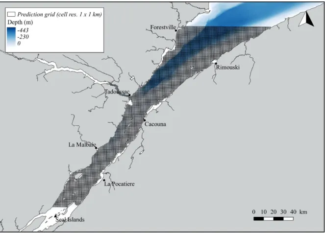
Figure 9. Distribution of the four marine mammal assemblages (k = 4) in the Lower St. Lawrence Estuary (LSLE). Assemblage 1 (n = 1,407) is shown in black, assemblage 2 (n = 1,175) in red, assemblage 3 (n = 993) in green and assemblage 4 (n = 437) in yellow. ... 39 Figure 10. Relative abundances of sightings (%) for assemblages 1 (n = 1,407), 2 (n = 1,175), 3 (n = 993) and 4 (n = 437). ... 40 Figure 11. Relative (grey bars) and cumulative (black curve) frequency (in %) of sightings for each species and assemblage. The dashed horizontal line indicates the number of species contributing to 80% of assemblages. ... 41 Figure 12. Proportions of sightings (%) of minke whales (n = 298), blue whales (n = 145), fin whales (n = 63), belugas (n = 631), grey seals (n = 492), humpback whales (n = 33), harp seals (n = 38), harbour porpoises (n = 2,255) and harbour seals (n = 57) in assemblages 1 (black), 2 (red), 3 (green) and 4 (yellow). ... 42 Figure 13. Predicted probabilities of assemblage membership of sightings estimated by multinomial logistic regression (MLR) for a) mean sea surface temperature over the 15 days previous to the sighting including survey date (SST15), b) mean sea surface salinity on survey date (SSS1), c) depth and d) slope. The x-axis of each plot represents the standardized values of variables (mean = 0, variance = 1). ... 47 Figure 14. Probable distribution of marine mammal assemblages based on the first (April) scenario of combined changes in mean sea surface temperature over the 15 days previous to the sighting including survey date (SST15) and mean sea surface salinity on survey date (SSS1). ... 49 Figure 15. Probable distribution of marine mammal assemblages based on the second (June) scenario of combined changes in mean sea surface temperature over the 15 days previous to the sighting including survey date (SST15) and mean sea surface salinity on survey date (SSS1). ... 50 Figure 16. Probable distribution of marine mammal assemblages based on the third (July) scenario of combined changes in mean sea surface temperature over the 15 days previous to the sighting including survey date (SST15) and mean sea surface salinity on survey date (SSS1). ... 51 Figure 17. Probable distribution of marine mammal assemblages based on the fourth (August) scenario of combined changes in mean sea surface temperature over the 15
days previous to the sighting including survey date (SST15) and mean sea surface salinity on survey date (SSS1). ... 52 Figure 18. Probable distribution of marine mammal assemblages based on the fifth (September) scenario of combined changes in mean sea surface temperature over the 15 days previous to the sighting including survey date (SST15) and mean sea surface salinity on survey date (SSS1). ... 53
INTRODUCTION GÉNÉRALE
La biodiversité à la base des services écosystémiques
La dégradation des écosystèmes naturels par l’homme menace de plus en plus la biodiversité des milieux terrestres et marins et met en péril leur équilibre fragile. À l’aube de 2020, pratiquement tous les écosystèmes de la planète ont été touchés par une ou plusieurs activités d’origine anthropique, et le déclin de centaines d’espèces a été enregistré dans la majorité des biomes (Butchart et al., 2010). L’utilisation excessive et la dégradation du territoire, les changements globaux, les espèces invasives, la surexploitation et la pollution sont les principales causes connues de ce déclin. L’importance de l’impact de ces vecteurs varie selon le type de vecteur, mais aussi en fonction des écosystèmes. Par exemple, la dégradation du territoire liée à la déforestation est le vecteur ayant le plus affecté les écosystèmes terrestres dans les dernières décennies, alors que la surexploitation liée aux pratiques de pêche mal ou non gérées a eu le plus grand impact sur les écosystèmes marins (Millennium Ecosystem Assessment, 2005). Confronté à l’une des plus grandes crises de la biodiversité qu’il ait connue, l’Homme n’a d’autre choix que de trouver des solutions, adaptées aux différents types d’écosystèmes, afin de préserver les richesses naturelles qui lui sont essentielles.
La biodiversité est à la base des services écosystémiques dont la race humaine dépend. Ces services relèvent de plusieurs catégories, allant de la production primaire à l’offre d’habitat, de l’approvisionnement en nourriture à la régulation du climat, etc. Une biodiversité élevée renforce la stabilité des écosystèmes. Les communautés biologiques présentant une biodiversité supérieure contiennent entre autres plus d’espèces clés ayant une influence positive sur la productivité des écosystèmes. À l’inverse, une perte de biodiversité peut réduire l’efficacité des communautés écologiques à capturer les ressources
biologiques essentielles, à produire de la biomasse et à décomposer et recycler les nutriments essentiels (Cardinale et al., 2012). La perte d’espèces diminue donc concrètement l’efficacité de fonctionnement d’un écosystème (Isbell et al., 2018).
Le milieu océanique et les préoccupations en matière de préservation de la biodiversité
Les écologistes terrestres reconnaissent depuis longtemps l’importance de la biodiversité comme indicateur de la santé et du bon fonctionnement des écosystèmes. La conservation des hotspots de biodiversité dans les écosystèmes terrestres est effectivement connue depuis longtemps comme un outil efficace de protection visant plusieurs espèces simultanément (Worm et al., 2003). Toutefois, à cause du peu d’attention accordée aux écosystèmes océaniques par rapport au milieu terrestre – ce dernier étant souvent plus accessible que son homologue marin, les connaissances sur la biodiversité marine sont largement incomplètes, ce qui fait que le lien entre la biodiversité et son incidence sur les écosystèmes marins est encore bien mal compris. Ceci empêche le développement de mesures de protection et de conservation crédibles et réellement efficaces. La nécessité de documenter davantage la diversité des espèces aquatiques devient urgente, surtout compte tenu des préoccupations liées au réchauffement climatique, à la dégradation des habitats et aux menaces anthropiques qui se révèlent de plus en plus complexes (Archambault et al., 2010).
L’importance des prédateurs apicaux en tant qu’outils de conservation
La biodiversité est une notion aussi vaste que complexe, et il est difficile de savoir comment s’y prendre pour la protéger. Mais, étant donné que les effets du déclin de la biodiversité sont au cœur d’un grand nombre de recherches depuis les 30 dernières années, plusieurs approches existent aujourd’hui afin de protéger la diversité biologique des écosystèmes (Cardinale et al., 2012). Certaines approches plus traditionnelles, par exemple,
sont centrées sur la protection d’espèces frôlant l’extinction et qui, de par leur profil dit plus « glamour », captent l’attention d’un plus grand nombre de gens (Scott et al., 1993). Mais en cette ère de défis de conservation grandissants, plusieurs s’entendent sur la nécessité d’adopter une vision plus globale afin de préserver la biodiversité sur une plus grande échelle. Une des alternatives possibles consiste à considérer plusieurs espèces à la fois, notamment les espèces dites représentatives. Celles-ci se retrouvent dans trois grandes catégories : les espèces fondamentales, indicatrices et parapluie. Les espèces fondamentales jouent un rôle essentiel dans la structure, le fonctionnement et la productivité d’un habitat. Leur rôle est souvent disproportionné par rapport à leur abondance. Les espèces indicatrices, elles, informent sur la santé ou la qualité d’un écosystème. Elles reflètent la présence d’autres espèces dans la communauté, mais reflètent également les changements dans l’environnement. Les espèces parapluie sont celles dont la protection entraîne aussi celle d’autres espèces qui fréquentent le même milieu (Simberloff, 1998). Le fait de concentrer les efforts sur ces espèces clés peut être bénéfique à la protection de la biodiversité, surtout si leur protection résulte par le fait même en la conservation d’un plus grand nombre de taxons (Walpole & Leader-Williams, 2002).
Les grands prédateurs apicaux – ces espèces situées aux plus hauts rangs du réseau trophique et qui, en général, se nourrissent principalement de vertébrés – ont toujours fasciné les humains. L’ours, le lion, le grand requin blanc et l’orque ne sont que quelques exemples d’animaux qui fascinent et inspirent le respect. Les scientifiques ont su exploiter la popularité de ces espèces comme levier d’action afin d’obtenir un support financier et accroître la sensibilisation du public. Mais le charisme de ces animaux n’est pas le seul facteur venant justifier leur protection : ces prédateurs peuvent réellement être considérés comme des espèces représentatives constituant des outils de conservation concrets et efficaces (Sergio et al., 2005). Sergio et al. (2008) ont publié une étude sur les liens entre les grands prédateurs et la biodiversité, et sur l’efficacité de leur protection en termes de bénéfices apportés aux écosystèmes. Selon eux, la présence de prédateurs dans un écosystème serait hautement susceptible d’entraîner une hausse de biodiversité en facilitant le flux de ressources et en déclenchant des réactions en chaîne causant une restructuration
des communautés. Et si la présence de prédateurs n’est pas toujours directement associée à une biodiversité accrue, elle semblerait au moins y être liée dans l’espace et dans le temps. Par exemple, la densité de carnivores terrestres (Carroll et al., 2001), de rapaces (Seoane et al., 2003; Sergio et al., 2003) et de prédateurs marins (Worm et al., 2003) a déjà été corrélée avec plusieurs paramètres de productivité écosystémique, qui eux, constituent des indicateurs de valeur de la diversité. De plus, les grands prédateurs sélectionnent généralement des habitats très complexes, où une forte biodiversité est favorisée par une combinaison de caractéristiques spécifiques. Les prédateurs apicaux sont également très sensibles aux perturbations de leur milieu (p. ex., pollution chimique, altération et fragmentation de l’habitat). Celles-ci sont susceptibles d’avoir un impact sur toute la communauté et donc sur la biodiversité de l’écosystème. Les prédateurs apicaux possèdent donc des qualités d’espèces fondamentales et indicatrices qui justifient leur protection, en raison, d’une part, de leur important rôle écosystémique, et d’autre part, de leur valeur en tant qu’espèces bioindicatrices. De plus, vu les exigences en termes de taille et d’interconnectivité de leurs aires d’alimentation et de reproduction, les grands prédateurs constituent d’excellentes espèces parapluie dont les besoins englobent ceux de plusieurs autres espèces (Roberge & Angelstam, 2004).
Le rôle des mammifères marins dans les écosystèmes océaniques
Les mammifères marins, groupe d’espèces englobant cétacés, pinnipèdes et siréniens, sont des organismes de grande taille hautement mobiles et vivant dans des environnements extrêmement dynamiques. Ils fréquentent tous les océans entre les deux pôles, et tous les types d’environnement, de côtiers à océaniques. Certains même se retrouvent dans les milieux d’eau douce. Ils occupent une large gamme de niches écologiques, ce qui leur confère une haute tolérance à un large éventail de conditions environnementales. Leur capacité de déplacement sur de longues distances, leur grande taille, leur abondance et leur taux métabolique élevé sont des facteurs qui contribuent à l’influence qu’ils exercent sur la
structure et le fonctionnement des écosystèmes marins (Harwood, 2001; Kiszka et al., 2015).
En raison de leur capacité à extraire d’énormes quantités de proies, ils ont une forte incidence sur la structure des communautés et la dynamique des populations qui se propage sur tout le réseau trophique (Bowen, 1997). À l’inverse, la grande taille des mammifères marins, en particulier de plusieurs espèces de cétacés, fait aussi d’eux des proies de choix pour plusieurs grands prédateurs, comme les épaulards ou les requins blancs par exemple, un détail important sachant que les ressources alimentaires en milieu océanique sont généralement dispersées et limitées (Roman et al., 2014). Les mammifères marins jouent également un rôle significatif dans le recyclage et le transfert horizontal et vertical de nutriments, et aident ainsi à maintenir la stabilité et la santé des océans. Lorsqu’ils plongent en profondeur pour s’alimenter et refont surface pour respirer, ils peuvent relâcher d’énormes panaches fécaux qui injectent dans les eaux de surface une quantité considérable de nutriments essentiels et limitants provenant des profondeurs. Cette facilitation de nutriments stimule la croissance du phytoplancton qui constitue la base du réseau trophique océanique (Roman & McCarthy, 2010).
Un grand nombre de mammifères marins, en particulier les cétacés, sont reconnus pour leurs longues migrations. Plusieurs espèces parcourent des milliers de kilomètres chaque année pour se déplacer entre les aires d’alimentation et les aires de mise bas, transportant ainsi de l’engrais, sous forme de fèces, d’endroits très productifs vers des endroits peu productifs. Le rôle de ces géants est également important après leur mort (Branch & Williams, 2006). Les carcasses de baleines, par exemple, constituent une source significative de détritus océaniques. Lorsqu’elles coulent au fond de l’océan, ces carcasses offrent une source de nourriture concentrée pouvant supporter une succession de communautés biologiques pendant plusieurs années voire décennies (Smith et al., 2015). Les ressources alimentaires étant très rares en haute mer, cet apport ponctuel fournit une partie importante de l’énergie nécessaire aux micro-organismes qui la réintroduisent ensuite dans le réseau trophique. Plus de 400 espèces, incluant charognards, détritivores et
bactéries, seraient associées à ces carcasses, et une trentaine de celles-ci seraient endémiques (Dahlgren et al., 2006; Smith & Baco, 2003). Pour toutes ces raisons, les mammifères marins contribuent à la bonne santé de leur environnement et constituent une composante essentielle des écosystèmes marins. La protection de ces grands prédateurs est fondamentale et essentielle à toute action visant à mieux préserver et favoriser la biodiversité de leur milieu.
Les mammifères marins et le Saint-Laurent
Le système hydrographique du Saint-Laurent représente une aire d’alimentation importante pour plusieurs espèces de mammifères marins du nord-ouest de l’océan Atlantique. La présence de nourriture abondante, stimulée par l’interaction favorable des conditions océaniques de l’estuaire du Saint-Laurent et de sa topographie accidentée, attire chaque année, de nombreuses espèces de poissons, d’oiseaux marins, et bien sûr, de pinnipèdes et de cétacés. La plupart de ces derniers effectuent d’importantes migrations annuelles, parcourant ainsi les dizaines de milliers de kilomètres qui séparent leurs aires de reproduction de leurs zones d’alimentation. Pour plusieurs, le Saint-Laurent représente une opportunité incontournable de s’approvisionner en nourriture et de reconstituer leur réserve de gras, indispensable pour le bon déroulement de leur cycle vital. Une vingtaine d’espèces de mammifères marins, incluant phoques, marsouins, baleines, rorquals et dauphins, sont recensées chaque année dans les eaux du Saint-Laurent, et près de la moitié sont fréquemment observées dans l’estuaire du Saint-Laurent, qui se trouve à plusieurs centaines de kilomètres de l’océan Atlantique.
Malgré cette impressionnante diversité d’espèces, les données quantitatives sur l’abondance et la distribution d’un grand nombre d’entre elles demeurent incomplètes, voire inexistantes. De plus, les sources d’information sont sporadiques, regorgent d’incertitudes et ne couvrent souvent qu’un secteur de l’estuaire ou du golfe du Saint-Laurent, ou une période restreinte de l’année (Gagné et al., 2013). Ce manque de
connaissances est entre autres lié aux divers défis posés par l’étude des espèces en milieu marin. En effet, les relevés visant la récolte de données sur les espèces marines sont souvent complexes et coûteux à organiser, en plus d’être grandement dépendants des conditions météorologiques. De plus, la grande variabilité dans les méthodologies utilisées entrave l’évaluation des tendances démographiques des espèces (Magera et al., 2013). Plus spécifiquement, les mammifères marins sont un des taxons de vertébrés les plus difficiles à étudier. Ils sont hautement mobiles et passent la majorité de leur temps sous la surface de l’eau. Certaines espèces sont solitaires, ce qui diminue grandement la probabilité de les détecter. De plus, l’environnement dans lequel elles vivent est vaste, et la plupart des espèces présentent des distributions qui s’étendent sur des milliers de kilomètres (Hunt et al., 2013).
L’insuffisance de données et de résultats interprétables représente un obstacle majeur aux prises de décision concernant la protection des mammifères marins de l’estuaire du Saint-Laurent, dont plusieurs espèces, notamment le béluga (COSEWIC, 2014) et le rorqual bleu (COSEWIC, 2012), qui ont un statut précaire. L’estuaire du Saint-Laurent est influencé par diverses pressions environnementales ou anthropiques; toutes les espèces de mammifères marins y passant une partie ou la totalité de leur cycle vital sont donc exposées à de multiples facteurs de stress (Williams et al., 2017). Ceux-ci incluent une importante navigation commerciale et récréotouristique, l’accumulation de contaminants industriels, la pêche commerciale, les changements climatiques et l’eutrophisation côtière (Dufour & Ouellet, 2007). Devant l’augmentation des activités humaines et leurs conséquences de plus en plus complexes sur les écosystèmes aquatiques, il devient urgent pour les organismes décisionnels de s’appuyer sur des connaissances et des avis scientifiques solides afin de limiter les dommages liés à ces activités (Savenkoff et al., 2017; Schloss et al., 2017).
Contexte, objectifs et hypothèses de l’étude
L’importance des mammifères marins pour le bon fonctionnement écosystémique de l’estuaire du Saint-Laurent est indéniable, mais mal comprise. Leur position dans le réseau trophique, leur rôle structurant ainsi que l’incidence positive qu’ils peuvent avoir sur la biodiversité de cet écosystème ne sont que quelques exemples qui poussent les scientifiques à recueillir un maximum d’informations sur ces espèces fondamentales afin de mieux les protéger, et par le fait même, de mieux protéger leur environnement. Ce projet de recherche constitue une pièce du casse-tête qu’est le concept de l’approche écosystémique, qui représente une solution possible aux problématiques de gestion liées à la détérioration des écosystèmes marins.
L’objectif principal de cette étude est de réaliser une analyse spatiale des assemblages de mammifères marins dans l’estuaire du Saint-Laurent. Plus précisément, il s’agit (1) d’approfondir nos connaissances sur la composition et la biodiversité des assemblages et (2) d’établir une corrélation entre leur distribution spatiale et les caractéristiques océanographiques de la zone d’étude, pour ensuite (3) générer un modèle prédictif et (4) produire des cartes de distribution des assemblages. Les analyses permettant d’exécuter ces étapes seront effectuées à partir d’une quantité considérable de données d’observations de mammifères marins recueillies lors d’une centaine de relevés systématiques effectués par bateau, et répétés dans une même zone d’étude et lors d’une même période de l’année et ce, pendant six saisons consécutives. Les cartes générées aideront à combler les lacunes causées par un manque de données important dans la région concernée. En effet, très peu de relevés, voire aucun, couvrent la totalité de l’estuaire, en particulier l’estuaire moyen, qui représente un habitat fréquenté par plusieurs espèces de mammifères marins, dont deux sont résidentes. Ceci limite notre compréhension de la distribution et de l’abondance de plusieurs espèces et freine le processus décisionnel en matière de gestion écosystémique.
L’hypothèse est que la distribution des assemblages de mammifères marins dans l’estuaire du Saint-Laurent est hétérogène et qu’elle est régie par certains paramètres environnementaux qui agissent étroitement sur la distribution et l’abondance des proies : la
température et la salinité de l’eau, la profondeur de l’eau et la topographie sous-marine. L’influence de l’environnement sur les espèces constituant les assemblages devrait être notée en examinant leur distribution, mais aussi en étudiant leur composition. Un faible chevauchement spatial entre les espèces est attendu, chevauchement qui devrait dépendre principalement d’espèces pélagiques peu motiles comme le zooplancton, d’espèces se nourrissant surtout de poissons pélagiques, et d’espèces se nourrissant essentiellement d’organismes démersaux. Les relations entre la composition des assemblages, la diète principale des espèces et les propriétés environnementales ayant une influence sut la distribution et l’abondance des proies des mammifères marins fréquentant l’aire d’étude devraient être suffisamment fortes pour prédire avec un degré de certitude relativement élevé la distribution spatiale des zones favorisant chaque type d’agrégation.
CHAPITRE 1:
SPATIAL ANALYSIS OF MARINE MAMMAL ASSEMBLAGES IN THE ST. LAWRENCE ESTUARY (CANADA)
1.1 INTRODUCTION
There is a well-documented loss of marine biodiversity worldwide, which is mainly due to human activities and their resulting pressures (Butchart et al., 2010; Jenkins & Van Houtan, 2016; Jones et al., 2007; McCauley et al., 2015; Tittensor et al., 2010; Worm et al., 2006). Human existence relies permanently on the oceans, and its impacts have increased over the past decades, mainly as a result of population growth, major developments in technology and numerous changes in land use (Halpern et al., 2008). Pressures on the oceanic environment are persistent and result from multiple usages and stressors, with the most notable ones including habitat degradation, overfishing and bycatch, toxic spills and climate change (Halpern et al., 2015). Marine mammals are threatened by all of them, directly or indirectly (Heithaus et al., 2008). Although accidental mortality through fisheries bycatch and vessel strikes are the two dominant threats, especially for species found in coastal areas, chemical pollution, noise, climate change and disease affect a great percentage of marine mammal populations (Schipper et al., 2008).
Marine populations and species are disappearing from ecosystems at a rapid pace as a result of pressures on the marine environment; in the case of marine mammals, at least 20% of species are currently considered at risk of extinction (IUCN, 2017). Marine mammals play a key role in ecosystems, shaping communities through predation and nutrient recycling (Bowen, 1997; Schipper et al., 2008; Smetacek & Nicol, 2005). Both cetaceans and pinnipeds are indeed important consumers occupying a variety of trophic niches. Their ecological significance is determined by their abundance and large body size, and is directly related to their potential to consume large quantities of prey (Kiszka et al., 2015). Marine mammals also contribute to nutrient cycling and enhance the productivity of ecosystems by feeding at depths and then defecating in the euphotic zone, and by
transferring nutrients downward to benthic communities through sinking of their carcasses after death (Lavery et al., 2014; Roman & McCarthy, 2010). Because of their generally important ecological role, the depletion of marine mammal populations can cascade into a series of effects on the ecosystem dynamics and structure (Harwood, 2001).
Less is known about marine ecosystem functioning when compared to terrestrial ecosystems, mainly as a result of logistical and financial constraints associated with research in this environment, where opportunities to conduct controlled experiments like those offered on land remain relatively rare (Archambault et al., 2010; Bowen, 1997). This has contributed to limiting our understanding of global patterns in species richness and their predictors (Tittensor et al., 2010). These data gaps, along with the challenges of implementing and enforcing conservation policies in the marine environment, likely contributed to the observed difference in protection levels between the two environments: oceans cover more than two thirds of the planet, yet less than 4% of the marine environment has received formal protection whereas 12% of the land is protected through national parks and reserves (Jenkins & Van Houtan, 2016). Data paucity is exacerbated in the case of marine mammals by their often wide-ranging movements, their vast distribution range, and the substantial amount of time they spend beneath the surface (Kaschner et al., 2011). In addition, some species are highly pelagic, spending their lives in offshore waters, away from the continents. As a result of these ecological factors, surveys dedicated to collecting data on marine mammal habitat use and distribution often cover only a fraction of their distribution range (Kaschner et al., 2006).
To effectively assess impacts of environmental pressures on marine mammals and aim for meaningful conservation efforts, the distribution of species in relation to their environment must be understood (MacLeod et al., 2008). With the development of high-speed computers and geographic mapping technology of the past decades, predictive ecological modeling became an inescapable research tool for quantifying species-environment relationships (Ovaskainen et al., 2017). Predictive distribution modeling is an associative method that relates occurrence or density data at known locations for a given
species (distribution data) to environmental characteristics of those locations (Gomez & Cassini, 2015). This geostatistical approach allows the interpolation or extrapolation of a few field observations to the entire potential range of a species and can be used for predicting the probability of species occurrence-based habitat suitability. It represents an attractive solution for getting around challenges related to data paucity (Rodriguez et al., 2007). Predictive modeling of species distribution exploits various methods and statistical techniques depending on the type of input data. Presence-absence data offer the greatest potential for robust model predictions. However, the widespread availability of presence-only data with no reliable information about absence locations has stimulated the development of methods exploiting this type of data (Pearce & Boyce, 2006). Predictive modeling serves two main purposes: identifying environmental drivers of species distributions and predicting distributions in hypothetical scenarios, assuming that the variables included in the model are relevant to species distribution and habitat use (Gomez & Cassini, 2015). Predictive modeling of distribution has a plethora of applications in conservation biology. In the absence of data, or in support of partial information on species habitat use and distribution, this approach has become an important research tool to assess the impact of environmental change on the distribution of species and to implement and prioritize conservation actions (Guisan & Thuiller, 2005). Maps generated by predictive modeling also help in forecasting where risk of interactions between human activities and species are likely to occur (Rodriguez et al., 2007). Modeling species responses to environmental predictors using presence-only data represents an appealing solution to the data paucity that is recurrently associated with wide-ranging or cryptic species such as marine mammals (Ready et al., 2010).
In general, species distribution modeling operates on a single-species basis, i.e., it assumes that species respond individualistically to changes in their environment (Bonthoux et al., 2013). However, the distribution of species is likely to be influenced by the distribution of other taxa, either through competition, predation or interspecific associations and relationships. These negative and positive associations between species can be captured by using level predictive modeling and may help better forecast
community-level responses and potential changes in biodiversity spatial patterns, especially at a finer scale (Elith & Leathwick, 2007). Species assemblages represent important features of an ecosystem that contribute to its structure, diversity and stability (Francis et al., 2002). They are also an important parameter in describing habitat diversity and richness that can help identify biologically and ecologically significant areas and inform management decisions (Chouinard & Dutil, 2011; Kenchington et al., 2011). Community-level predictive distribution modeling can be done using three broad strategies. The first one consists in grouping species into assemblages first, and then modeling the distribution of these assemblages. A second strategy consists in predicting the distribution of individual species first, and then grouping these species into assemblages. The third strategy involves joint modeling of individual species and species assemblages (Chapman & Purse, 2011). The first approach was used in this study since it allowed using all the sightings, including those of species rarely observed, and explicitly accounted for species occurrence or co-exclusion (Ferrier & Guisan, 2006).
Modeling of community or assemblage responses to environmental factors has been conducted for a variety of species including benthic organisms (e.g., Degraer et al., 2008; Moritz et al., 2013), birds (e.g., Hyrenbach et al., 2007; Woehler et al., 2003), fish (e.g., Chouinard & Dutil, 2011; Tamdrari et al., 2015), insects (e.g., Dufrêne & Legendre, 1997; Kremen, 1992), mammals (e.g., Ahumada et al., 2011; Hortal et al., 2008) and plants (e.g., Ackerly & Cornwell, 2007; Lortie et al., 2004). Many have explored the usefulness of species assemblages as indicators of biological diversity and integrity, but despite this increasing interest for community-based research, little has been done to study the distribution of marine mammal assemblages due to the difficulty of gathering sufficient data. Examples of studies about the structure of marine mammal communities include work from (Baumgartner et al., 2001) who examined the distribution of five cetacean species groups in the Gulf of Mexico, from (Hamazaki, 2002), who constructed a cetacean habitat model in the mid-west North Atlantic using sightings from 13 cetacean species, and from (Schick et al., 2011), who used community ecology analyses to uncover the structure of pelagic marine mammal communities in three different areas of the western North Atlantic.
The St. Lawrence Estuary (SLE) is a productive area in Eastern Canada, where several species of marine mammals are known to occur either year-round or on a seasonal basis (Savenkoff et al., 2017). It is located downstream of industrialized areas and represents the main waterway to central North America in addition to supporting a multimillion-dollar whale-watching industry. Human pressures are numerous in this environment, and could be cumulative (Schloss et al., 2017), leading to habitat degradation through noise and disturbance, chemical contamination, and for some species, reduced availability of food resources as a result of fishing or climate variability (DFO, 2014; Lesage et al., 2017; Simard et al., 2010; Williams et al., 2017). Habitat use by the various species of marine mammals occurring in the SLE is currently poorly described (Lesage et al., 2007).
The objectives of this study were to use marine mammal presence-only data obtained during systematic line transect surveys in the SLE in order to: (1) explore, using multivariate analyses, the composition and distribution of marine mammal assemblages in the SLE, (2) describe the relationship between the probability of occurrence of each assemblage using environmental factors and community-level predictive modeling, and (3) predict the probable distribution of assemblages over a larger area of the SLE using multinomial logistic regression and changes in distribution according to scenarios of varying temperature and salinity.
1.2 METHODOLOGY
1.2.1 Study area
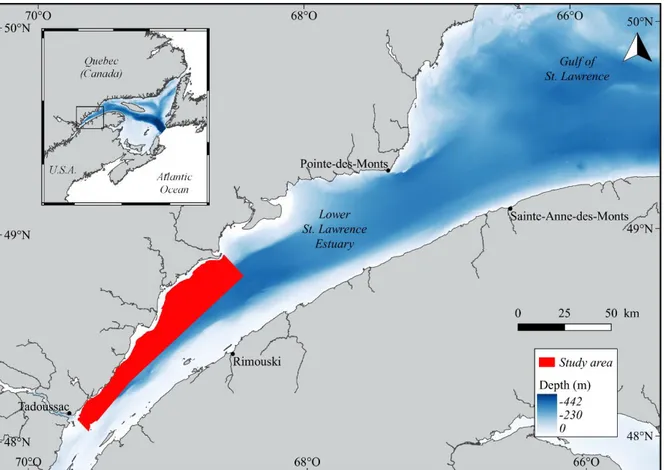
This study was conducted in the St. Lawrence Estuary, Canada, more specifically in the Lower SLE (LSLE), a 200 km long, 40 km wide body of water that extends from the mouth of the Saguenay Fjord, near Tadoussac, downstream to Pointe-des-Monts/Sainte-Anne-des-Monts, the western limit of the Gulf of St. Lawrence (GSL) (Figure 1). Due to its dimensions and major connections to oceanic waters, the LSLE is considered as a marine environment (El-Sabh & Silverberg, 1990). The Laurentian Channel (LC), a 350 to 450 m deep canyon that runs from the Atlantic Ocean off the continental shelf all the way through the LSLE, establishes a major link between the two environments, influencing the circulation, mixing and characteristics of water masses (Lavoie et al., 2000). The LC ends abruptly at the confluence of the Saguenay Fjord and the SLE, resulting in an upwelling of cold mineral-rich waters and enhanced productivity that attracts several marine species, including at least twelve species of marine mammals (Savenkoff et al., 2017). The beluga (Delphinapterus leucas) and the harbour seal (Phoca vitulina) are known residents of the SLE, although a portion of these populations seasonally migrate east into the GSL (Lesage et al., 2004; Mosnier et al., 2010).
Figure 1. The Estuary and Gulf of St. Lawrence, Eastern Canada. The area where this study took place (in red) is located in the Lower St. Lawrence Estuary (LSLE).
1.2.2 Surveys and marine mammal sightings
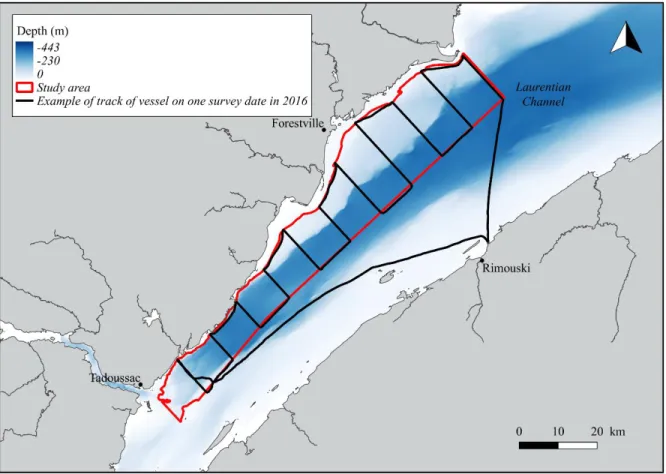
Vessel-based surveys of the northern portion of the LSLE, including the LC (Figure 2), were conducted weekly (weather permitting) between April and November of 2009 through 2014. Start and end dates of surveys in the spring and fall varied between years according to ice conditions. The survey platform was a 32 feet long rigid hull zodiac (the Cetus) equipped with a cabin and a flying bridge where two observers were posted. Surveys covered an area of approximately 980 km2 on average, and followed a systematic line transect design with a random start point for each survey. Transects were limited to waters 10 m deep or more. They were oriented across bathymetry gradients, were spaced by 7 km,
and were 13 km long on average. This sampling design afforded all points in the study area an equal probability of being sampled (Buckland et al., 2001).
Figure 2. Typical sampling design on a survey day in the Lower St. Lawrence Estuary (LSLE). The red line delineates the area in which surveys were done. The black line is an example of a track followed by the research vessel. Observers were on effort when surveying perpendicular to the coast; only opportunistic sightings were collected during transits between transects (parallel to the coast) and these were not included in the analysis. Depth data were obtained from a 50 m resolution raster created by interpolating data from the Canadian Hydrographic Service.
Observers varied between survey days and years, given the time span of this study. However, they were trained by experienced observers over multiple surveys before being considered as primary observers. All aquatic megafauna species encountered were recorded; sightings of sea turtles, sharks or tunas were highly infrequent and were not
considered here. Observers recorded information on audio tape recorders and searched for megafauna primarily with the naked eye, and periodically using binoculars. They noted the species, number of individuals (young and adults combined), time, relative angle of the sighting with respect to the heading of the vessel, and relative distance using primarily reticules in the binoculars, or naked eye when the sighting was within 50 m from the survey platform. Weather conditions (sea state, sun glare intensity, cloud cover and visibility) were also recorded at the beginning and at the end of each transect, or as they changed during transects. Information on relative distance and angle from the vessel were used to position each sighting. Only sightings of positively identified species were retained for the analyses.
1.2.3 Environmental data
When predicting the spatial or temporal distribution of wildlife, it is always best to rely on ecological parameters believed to be the driving forces of their distribution (Guisan & Zimmermann, 2000). Prey availability is the variable most likely to affect marine mammal distribution during the foraging season (Baumgartner et al., 2001). In the LSLE however, the near-absence of fishing activities has resulted in little scientific effort being steered toward monitoring invertebrate and fish abundance and distribution (Mosnier et al., 2016). While data exist for some species, there was a mismatch in the temporal and spatial resolutions of the available data on prey species distribution and abundance and the data on marine mammal occurrence collected during the systematic surveys. Because the aggregation and distribution of zooplankton and fish are often driven by physical environment properties, abiotic variables can be used as a proxy for prey distribution (Torres et al., 2008). For the subsequent analyses, such variables were selected considering their likely ecological significance for marine mammal occurrence as well as data availability (Correia et al., 2015).
Four environmental variables were gathered from different sources. Depth was obtained from a 50 m resolution raster created by interpolating data from the Canadian
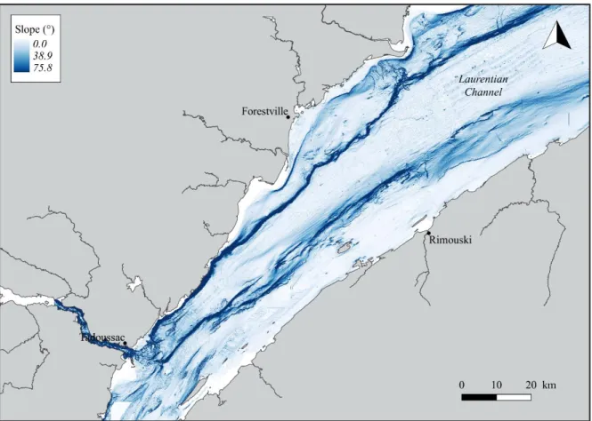
Hydrographic Service (Figure 2). Bottom changes in topography (slope) were derived from the same raster by calculating the maximum rate of change (in degrees) in depth between neighbouring cells (Figure 3). Data for these two variables were extracted and compiled for each georeferenced sighting recorded during the 2009 to 2014 observation period.
Figure 3. Bottom slope (in degrees) of the Lower St. Lawrence Estuary (LSLE) computed from depth data obtained from a 50 m resolution raster created by interpolating data from the Canadian Hydrographic Service.
Predictive models combining static (e.g., depth and slope) and dynamic variables (variables that change over the timeframe being modeled) tend to perform better than models based on static variables alone (Ballance et al., 2006). Therefore, sea surface temperature (SST) and salinity (SSS) were added because they may represent good proxies for species distribution in marine habitats (Correia et al., 2015; Redfern et al., 2006). These
parameters were not collected during the surveys, so other available sources, including remotely sensed data and models of oceanographic processes, were exploited. Data on SST were extracted from NOAA’s Advanced Very High Resolution Radiometer satellite images (~ 1.1 km resolution; available at ogsl.ca). Eleven different values of SST were considered: mean SST over the 1, 3, 5, 7 and 15 d previous to the sighting including survey date, 3 and 5 d means centered on the survey date, and 3 d means with a 3, 5, 7 and 15 d lag from the survey date. Collinearity among these variables was examined using Pearson’s correlation coefficients (r). SSTs with r > 0.5 were considered correlated and the SST value with the least amount of missing data was kept while the others were removed from the dataset. SSS at the sighting location was estimated (~ 6 km resolution) from an oceanographic model for each survey date (Saucier et al., 2009; Saucier & Chassé, 2000). Sightings with missing data on one or more environmental variables, which represented < 1% of the initial data, were eliminated from the dataset. Environmental variables (depth, slope, SST and SSS) were standardized (mean of 0, variance of 1) to avoid biases associated with discordant scales.
Other variables potentially useful for describing marine mammal habitats were not included in the analysis as they were limited in their spatial resolution and distribution, and would have resulted in the loss of a high number of sightings. These variables included surface and subsurface water properties (i.e., depth of thermocline, mixed layer and euphotic zone, sea surface dynamic height, frontal regions), water conditions or index of productivity (i.e., fluorescence, chlorophyll a, dissolved oxygen content, water color), bathymetry (i.e., distance to shelf edge, distance to shore) and prey availability (Dransfield et al., 2014; Redfern et al., 2006, 2017). Other variables, like depth of the cold intermediate layer and euphotic zone, sea level anomalies, oceanic fronts and sediment grain size were explored for inclusion in a previous study specifically examining beluga habitat but were discarded for various reasons (see Mosnier et al., 2016).
1.2.4 Statistical analysis and modeling framework
Species presence-only data were used to model assemblage distribution as opposed to species abundance. The presence of certain constraints regarding the size of the study area, the resolution of environmental layers used as background data, and the number of marine mammal sightings made presence-only data the optimal data to use in order to reach our research objectives. Results of occurrence models are still considered as good indicators of variations of species abundance, and these models do reflect environmental suitability, where more taxa should inhabit most suitable areas (Estrada & Arroyo, 2012).
Marine mammal assemblages in the LSLE were identified using a hierarchical cluster analysis performed on the environmental data and based on a dissimilarity matrix. Ward’s minimum variance agglomeration method (Ward, 1963) was preferred over other common linkage methods as it is less susceptible to be distorted by outliers (Blashfield, 1976; Hands & Everitt, 1987; Kuiper & Fisher, 1975). The Euclidean distance was chosen over non-Euclidean distances or dissimilarity measures such as the Bray-Curtis dissimilarity index, the Manhattan distance or the Jaccard index because the analysis was performed on the similarity of sightings (presence data) in relation to environmental variables that described them, and not on species abundances.
Three methods were used to identify the appropriate number of clusters for describing our dataset on marine mammal sightings. First, a static tree cut method was applied to define separate clusters as contiguous branches below a fixed height cut-off (Langfelder et al., 2008). Second, total within-cluster sum of squares was calculated for the k possible clusters, and k with the smallest sum of squares was selected as the appropriate number of clusters. Finally, the choice of the appropriate number of clusters was validated using Hubert’s statistic, a graphical method in which one searches for a significant peak of second differences, which corresponds to the relevant number of clusters in a dataset (Charrad et al., 2014; Hubert & Arabie, 1985).
An analysis of group similarities (ANOSIM) with 4,999 permutations was performed to verify that observations in the various clusters differed in their environmental characteristics, i.e., to determine whether the assemblages displayed different environmental characteristics. Between-cluster differences for each of the environmental variables were examined using univariate Kruskal-Wallis rank sum tests, and specific clusters differing in characteristics were identified using pairwise comparisons and Bonferroni-corrected post hoc Wilcoxon rank sum tests.
Clusters of observations, hereafter referred to as assemblages, were then described in terms of species composition, dominant species and biodiversity. The proportions and relative abundances of sightings (percentages of sightings of one species in each assemblage and percentages of sightings of the various species in a given assemblage, respectively) were considered. Variations in the proportion of sightings of each species within each assemblage were also tested with Pearson’s Chi-squared tests. Dominant species were assessed by comparing their relative abundances of sightings in each assemblage. Assemblage biodiversity was considered in three ways: species richness, diversity and evenness. Species richness (S) is the total number of species. Species diversity was measured using Shannon’s diversity index (H’), which considers the relative frequency of each species, as well as the number of individuals for each species. Species evenness, referring to how evenly the individuals are distributed across species, was measured using Pielou’s evenness index (J) to analyze the uniformity of assemblages (Magurran, 2004).
Multinomial logistic regression (MLR) was used to predict the probability of a sighting falling into a given assemblage given its characteristics in terms of the following four independent continuous variables (X): mean SST over the 15 days previous to the sighting including survey date (SST15), mean SSS on survey date (SSS1), depth and slope. MLR is an extension of a logistic regression, where the response variable (Y) is nominal, i.e., it has multiple categories (k > 2) that cannot be ordered in any meaningful way. When
k > 2, there are k * (k - 1) / 2 logit functions that can be formed, of which only (k - 1) are
response variable, where coefficients are estimated using maximum likelihood, as opposed to an ordinary least square estimator. The choice of the pivot category does not affect the estimated coefficients, calculated probabilities or significance of variables (Menard, 1995).
In our study, the outcome variable had four categories; therefore, there were three equations following the same generic structure, in which the log of the odds ratios were calculated for all other categories (assemblage 2, 3 or 4) relative to the pivot category (assemblage 1), resulting in a linear function of the predictors:
𝑙𝑛 (𝑃𝑟𝑜𝑏. 𝑌
𝑃𝑟𝑜𝑏. 1) = 𝛽0+ 𝛽1(𝑆𝑆𝑇15) + 𝛽2(𝑆𝑆𝑆1) + 𝛽3(𝐷𝑒𝑝𝑡ℎ) + 𝛽4(𝑆𝑙𝑜𝑝𝑒)
All models with a combination of one to all variables were tested. The multinom function from the nnet R package (Venables & Ripley, 2002) was used for MLR estimations. Selection of the model best predicting observations was based on the Akaike Information Criterion (AIC) where the best model was the one with the lowest AIC (Akaike, 1974). The relevance of each environmental variable was examined by leaving one variable out at a time and by comparing residual deviances of resulting models with the optimal model. The predictive performance of the selected model was tested by running the MLR on a “training” dataset composed of 3,212 randomly selected sightings from the main dataset, representing 80% of the sightings. The accuracy of predictions about assemblage membership was tested using the remaining 800 observations by comparing model predictions with the observed assemblage assignments and estimating classification error rates.
MLR makes no assumption about the relationship between the dependent and independent variables, the distribution of data, the errors or the variance. However, MLR makes the assumption of observation independency and may be sensitive to multicollinearity and to small sample size given that MLR uses maximum likelihood to estimate regression parameters (Quinn & Keough, 2002). Given that all assumptions can rarely be met in empirical data, validation of model predictions is often performed using an independent source of data.
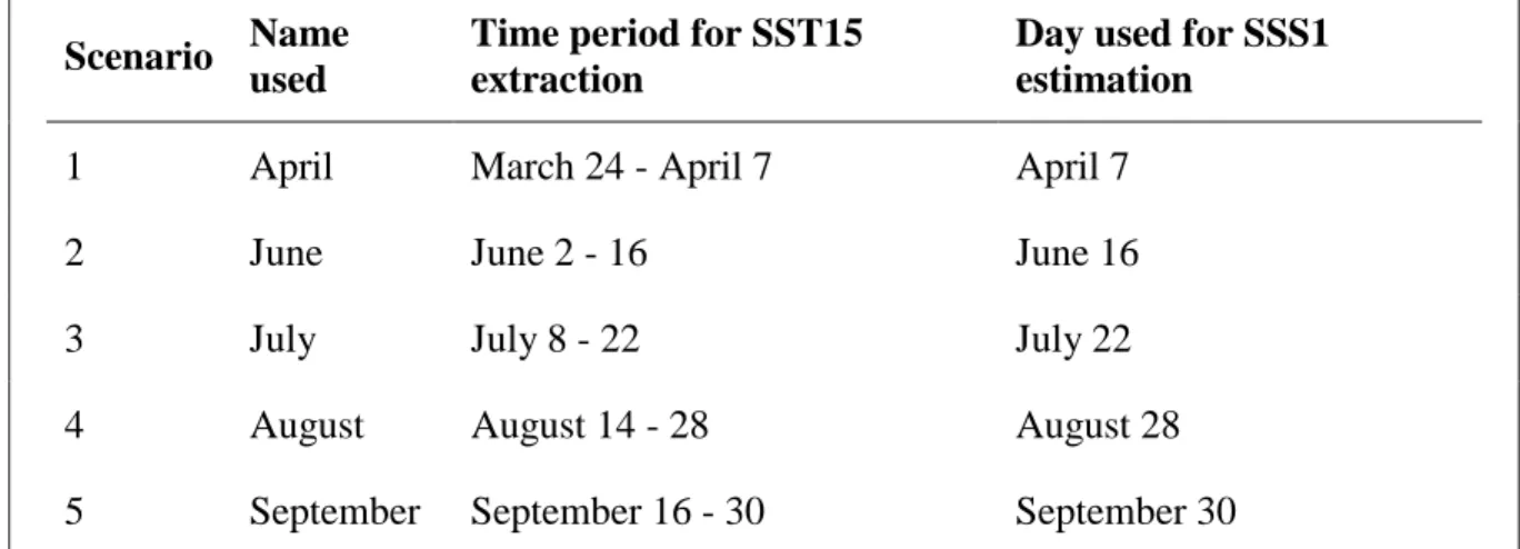
Model predictions, i.e., probability of a sighting being assigned to a given assemblage considering the selected environmental characteristics, were plotted on a 1 km grid cell covering the SLE from the area north of Seal Islands in the Upper SLE and Forestville in the LSLE (Figure 4). This was done for five scenarios, in which values of SST and SSS changed, to assess the effect of the variability in dynamic variables on model predictions. SST (15 d means) was extracted for five time periods in 2014 (Table 1). SSS (1 d means) of the last day of each time period was estimated using an oceanographic model (refer to section 1.2.3 for methodology on the extraction of SST and estimation of SSS). In each scenario, cells of the prediction grid were attributed the value of each predictor variable at the cell centroid. Cells with a centroid located on land were deleted from the prediction grid. Data were analyzed using R version 3.4.1 (R Core Team, 2017). Geographical distribution of marine mammal assemblages was mapped using ArcGIS software (version 10.2, ESRI Inc.).
Table 1. Names, time periods and days used for the extraction of mean sea surface temperature over the 15 days previous to the sighting including survey date (SST15) and estimation of mean sea surface salinity on survey date (SSS1) for the five scenarios used to model assemblage membership for each 1 km cell of the prediction grid.
Scenario Name used
Time period for SST15 extraction
Day used for SSS1 estimation
1 April March 24 - April 7 April 7
2 June June 2 - 16 June 16
3 July July 8 - 22 July 22
4 August August 14 - 28 August 28
1.3 RESULTS
1.3.1 Marine mammal sightings
Between 11 and 25 weekly surveys were completed each year between April and November, mainly between May and October, resulting in 100 surveys for the period of 2009 to 2014, and 4,029 sightings of nine marine mammal species (Figure 5a). Species included baleen whales [minke whales (Balaenoptera acutorostrata), blue whales (Balaenoptera musculus), fin whales (Balaenoptera physalus) and humpback whales (Megaptera novaeangliae)], odontocetes [belugas (Delphinapterus leucas) and harbour porpoises (Phocoena phocoena)], and pinnipeds [grey seals (Halichoerus grypus), harp seals (Pagophylus groenlandicus) and harbour seals (Phoca vitulina)] (Figure 6).
Figure 5. a) Number of surveys per month, and b) effort-corrected seasonal change in the number of sighted individuals (light grey bars) and sightings (dark grey bars) (± SD).
Figure 6. Spatial distribution of sightings of a) baleen whales (n = 549), b) odontocetes (n = 2,891) and c) pinnipeds (n = 589).
The number of sightings and individuals per survey shows a progressive increase in marine mammal occurrence in the LSLE from April through July and August, followed by a progressive decline from September through November (Figure 5b). This trend was mainly driven by odontocetes, which comprised the most abundant species group (see below), but also by pinnipeds (Figure 7). Baleen whales increased in mean occurrence per survey from April through June and remained present at constant levels until October after which their occurrence declined.
Based either on the number of sightings or sighted individuals, harbour porpoises were by far the most commonly observed species in the LSLE, followed by belugas and grey seals (Table 2). Humpback whales and harp seals were the least frequently observed
species. Mean group size differed among species, with harp seals and belugas being observed mostly in groups. Occasionally, groups of several tens of grey seals were encountered at sea, contributing to increase the variance in group size for this species. Harbour seals and minke whales were generally observed on their own.
Figure 7. Seasonal change in the mean number of sightings per survey presented by species group (± SD).