Science Arts & Métiers (SAM)
is an open access repository that collects the work of Arts et Métiers Institute of Technology researchers and makes it freely available over the web where possible.
This is an author-deposited version published in: https://sam.ensam.eu Handle ID: .http://hdl.handle.net/10985/10921
To cite this version :
Guillaume MARTIN, Etienne BALMES, Guillaume VERMOT DES ROCHES, Thierry
CHANCELIER - Review of model updating processes used for brake components - In: Eurobrake, Allemagne, 2015-05 - Eurobrake - 2015
Any correspondence concerning this service should be sent to the repository Administrator : [email protected]
EB2015-ADS-001
REVIEW OF MODEL UPDATING PROCESSES USED FOR BRAKE
COMPONENTS
1,3
Martin, Guillaume*; 1,3Balmes, Etienne; 1Vermot-Des-Roches, Guillaume ; 2Chancelier, Thierry
1
SDTools, France; 2Chassis Brakes International, France; 3Arts & Metiers ParisTech, France KEYWORDS – Model updating, Geometry errors, Modal Correlation, Material parameters, Contact properties
ABSTRACT - To be confident in the prediction capability of a model, verification and validation steps are classically performed. Verification checks that the model is properly solved. Since the model used are fairly standard, this is not issue for brake components. Validation checks the relation between model and experiments on actual structures. Here geometry measurements and vibration tests are considered. The study seeks to perform a systematic review of how test quality is evaluated, and models are correlated and then updated. This will give a solid basis to define clear and easily used validations protocols for brake components where prediction of modes and their stability in the manufacturing process is often deemed critical.
Updating the geometry before updating the material properties is shown to be very important: the residual error on frequencies is smaller and no bias is introduced in the estimated material properties. Proper pairing of modeshapes is important for broadband comparisons and the MAC criterion is used. Intermediate steps: experimental topology correlation using easy tools with accuracy evaluation, estimation of errors on test shapes, handling of mode crossing, are sources of errors that are analyzed.
For the updating of contact properties, where many parameters may need update, the use of model reduction is shown to allow a major speed-up of parametric studies.
INTRODUCTION
While the process of updating components then assemblies is fairly often proposed, it is not very often fully applied. The main motivation of this paper is a review of typical difficulties in the model updating process with a focus on illustrating each difficulty and analysing the sources of error on both the model and the test sides. The aim behind this study is to orient the development of an easy and accurate validation protocol for brake components which could then be more systematically applied.
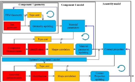
Validation and model updating has been decomposed in three steps, illustrated in Figure 1. Component geometry has been found to be critical and is first addressed. From a cloud of measured points, one either reconstructs a CAD geometry and remeshes or morphs the nominal FEM mesh (1). Once an accurate component geometry obtained, density is updated from weight measurements and elastic properties are adjusted from paired modal frequencies obtained through an experimental modal analysis. Once components updated, the next level is assemblies which are verified in multiple stages where different components are connected. The only parameters associated with assemblies are contact surfaces and/or contact stiffness, whose choice will be discussed. Assembly validation is performed by correlating numerical and test modeshapes of the assembly at a given stage.
Figure 1 : Updating protocol: component geometry, component properties, contact properties of assemblies.
The case of a drum brake plate, assembled with its fixed point and cable guide shown in Figure 2, will be used to illustrate the key issues of the proposed protocol. Section 1 illustrates the strong influence of geometry and thus the need of geometry updating by comparing
frequencies and modeshapes for the nominal CAD and a reconstructed geometry. Section 2 then focuses on the classical Young modulus updating using error on frequencies. It is in particular shown that skipping the geometry updating induces a bias in the estimated parameters.
While modal order may be sufficient to pair modes of a component and update its modulus, this is often wrong for assemblies and shape correlation is typically needed for a proper correlation of test and FEM modeshapes. Section 3 discusses topology correlation, the step in which FEM and modal test wire-frame geometries are matched to allow computation of the classical Modal Assurance Criterion (MAC). In the particular case of interest, tests are performed using 3D vibrometer testing which generates large sensor counts. It is thus shown how automated sensor set selection can be introduced and gives better accuracy in the correlation.
Section 4 finally addresses assemblies. Modelling strategies, where both contact surface and stiffness are considered, are illustrated for two contact surfaces present here: fixed point/plate and fixed point/cable guide. Reduced order models are used to allow fast computations of the evolution of correlation for variable contact parameters.
Figure 2 : Drum brake plate, cable guide and fixed point components to be updated
Plate
Cable guide
Fixed point
1. COMPONENT GEOMETRY UPDATING
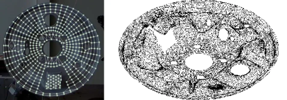
The updating of geometry is based on the measurement of a physical component which provides a very dense point cloud (see Figure 3). From this point cloud, two ways to rebuild a geometrically accurate model were considered. The first is to reconstruct a CAD geometry directly from the measured point cloud (no initial FEM needed here) and mesh the obtained volume. A second possibility is to mesh the nominal CAD geometry and then morph the mesh to have surface nodes on the point cloud. Both techniques have been applied with currently no clear winner and rapid evolutions of both. The objective here is to illustrate the need to use updated geometries.
Figure 3 : COMET Steinbichler 3D Structured Light Scanner
For the illustration, the nominal and reconstructed CAD are meshed using the same
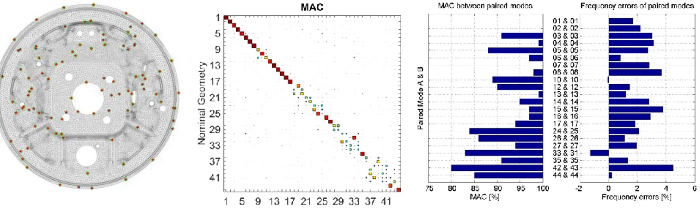
parameters (quadratic tetrahedra, minimum characteristic length of 2 mm and maximum of 3 mm). Using the same steel parameters, modes are computed and need to be compared. Since meshes are not compatible, the two geometries are superposed (see Section 3 for details) and the algorithm developed by Balmes et al. (2) is used to place representative points allowing accurate differentiation of modes of the nominal model. Figure 4 left shows the locations of these points.
Figure 4 middle shows that the MAC between the two modeshapes are well correlated until mode 17 (3200Hz) except for modes 9 and 11 which are below 70%. But since these modes are close in frequency, mode switching can be suspected. Above 3200 Hz, some modes are well correlated but many of them differ notably. The nominal FEM also has higher
frequencies (a mean of 2%), as shown in Figure 4 right.
Figure 4 : Nominal/Reconstructed modeshapes comparison: Compared locations (left), MAC between the two sets of modeshapes (middle), MAC and frequencies errors of paired modes (right)
These differences are quite significant and clearly illustrate the need to update the geometry before attempting any property update.
2. UPDATING OF COMPONENT MODEL PARAMETERS
Once the geometry updated, the next step is to adjust component parameters. The first step is to adjust the density. Since the volume is now properly known, a simple weighing is used. The second step is an adjustment of the elastic properties. In general for metallic parts, the Young modulus would be considered. If the component has a complex geometry, modeshape pairing may be needed and this will be discussed in section 3. But since component models are fairly accurate, simple modal ordering is often relevant at least in the low frequency range. For the case of the plate, collocated transfers were measured using an impact hammer and an accelerometer. As shown in Figure 5 left, points are chosen to allow proper identification of most modes.
Figure 5 : Collocated transfer identification (left) and mass shifting (right)
The right image, illustrates that mass loading due to the accelerometer is of importance for some modes. Here for mode 8 at 2005 Hz, one has frequency shifts of the order of 0.3 % for a bandwidth 0.12%. Measurements must thus be analysed separately thus introducing the difficulty of rematching modes in each measurement. Contactless methods such as laser vibrometers may be difficult to use in applications, where many components are tested in a plant. Automating the handling of mass shift effects is thus a requirement and error
evaluations tools (3) may be of interest.
Assuming paired mode and low mass loading, one defines a relative error on frequencies 𝐽(𝐸) = mean (|∆𝑓𝑖|
𝑓𝑖 (𝐸)) and updates the Young modulus to minimize this cost function.
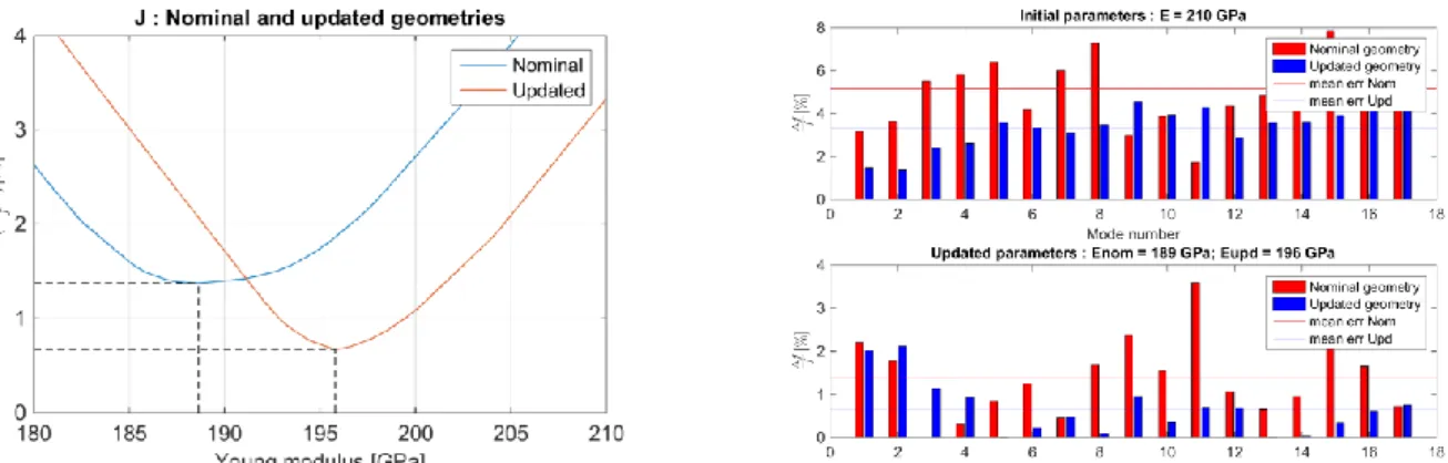
Figure 6 illustrates the evolution of the cost function for the nominal and updated geometries. Associated errors on frequencies are also detailed in the figure. First, it clearly appears that errors are notably smaller for the updated geometry. The mean error is 0.8% rather than 1.3%. The standard deviation of frequency errors is also lower (0.6% rather than 0.9%). Then, the example shows that skipping the geometry update would lead to a bias in the modulus estimate. One would find E=189 GPa rather than the more realistic 196 GPa.
Figure 6 : Cost function for nominal and updated geometries (left); Relative error of each modes before and after the young modulus updating
3. EFFICIENT MODESHAPE CORRELATION
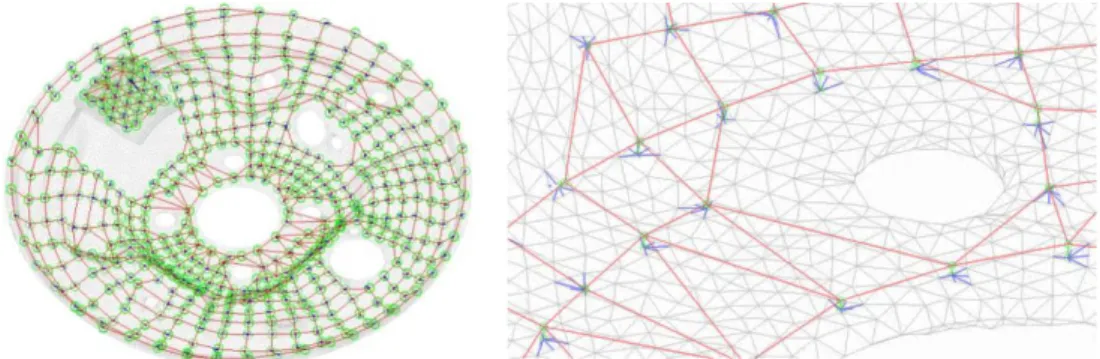
For assemblies, it is generally necessary to pair modes for proper comparison. Extracting and comparing test and FEM shapes is thus necessary. Experimental Modal Analysis (EMA) of brake components are, at CBI, typically performed with a 3D laser vibrometer equipped with a geometry scan unit which gives the topology of the scanned points, shown in Figure 7 left. On the FEM geometry, one only keeps the skin visible from the measurement point of view. This disables the possibility to match parts of the scan on undesired surfaces which can lead to local minimum in the optimization process.
Figure 7 : Test wireframe (left) and FEM geometry (right)
Because the superposition will be the result of an optimization, the first step is to initialize the relative position. To do so, one manually gives at least three corresponding points between the FEM geometry and the test wireframe. The distance between these paired points is minimized and an initial position is defined.
From this position, one uses an Iterative Closest Point algorithm, and more specifically, the point-to-surface variant to optimize the relative position. The advantages of the point-to-plane variant are that it converges faster than the point-to-point algorithm and can be linearized assuming small displacements (4) (5). Figure 8 shows at the left the initial relative position (with three paired points given). After the optimization with the ICP point-to-plane algorithm, one sees that the mean error and standard deviation is much lower, and the optimization process is quite fast: less than one second for 300 points in the test wireframe. To superpose the two FEMs geometries in Section 1 (the scan and the nominal geometry) which count about 200 000 nodes each, it only takes 10 seconds.
No optimization, 0.39 seconds mean error = 1.14 mm
std error = 0.88 mm max error = 5.34 mm
Optimization : 7 iterations in 0.69 seconds mean error = 0.82 mm
std error = 0.58 mm max error = 3.01 mm
Figure 8 : Superposition of the test Wireframe over the FEM geometry: initial state (left) and optimized position with ICP point-to-plane (right)
Once the optimized relative position is reached, one builds the observation matrix of the FEM to observe deformations at the location of sensors in the test wireframe. Each test wireframe node is projected on the closest FEM surface and deformations of the FEM modeshapes at these locations are obtained from interpolation using elements’ form-functions.
Figure 9 : Observability matrix building
With the use of the ICP algorithm, the step of superposition, which can be quite difficult and time consuming to do manually, is speeded-up and one has easily access to criterion on the quality of topology correlation. One has now two coherent sets of modeshapes that can be compared, classically with the Modal Assurance Criterion.
Modeshapes are identified from the Experimental Modal Analysis measurements, Numerical modeshapes are observed with the previously defined observability matrix and the MAC is computed (see Figure 10).
Figure 10 : MAC between EMA and Assembly modeshapes (left), Frequency errors of paired modes (right)
The quality of the match between the FEM model and the test wireframe is of great
importance to be confident on the correlation evaluation. Taking the two relative positions in Figure 8 (before and after the ICP optimization) and computing the observation matrix and the MAC, Figure 11 shows that the correlation is much better after the optimization.
Figure 11: MAC with and without ICP optimization
Using a 3D Laser gives the advantages of a non-contact measurement (no mass loading as with accelerometers) and a lot of points can be measured. Nevertheless, when the response of the structure is low, especially in in-plane directions, or in case of measurements on inclined surfaces, signals may be very noisy. Even if noise occurs mostly at small displacement locations, it is sometime not neglectable and can contribute to a poor correlation. To take this
into account, we want to create for each identified modeshapes a set of well identified sensors which will only be used to compute the MAC. To automatically create this sensor sets, we introduce the MAC-error criterion (3)
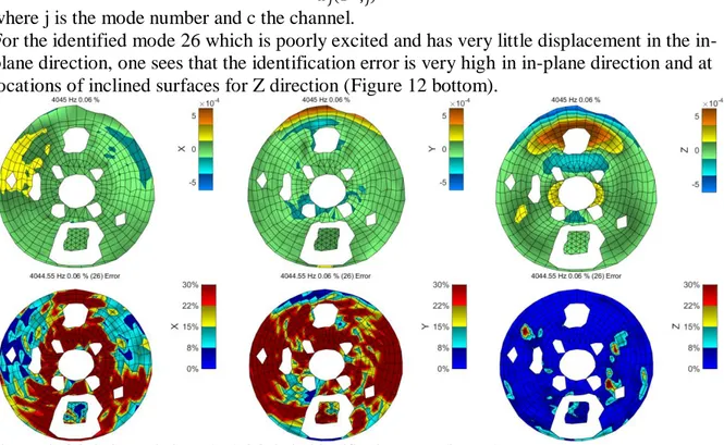
𝑒𝑗,𝑐 =∫ |𝐻𝑇𝑒𝑠𝑡,𝑐(𝑠) − 𝐻𝑖𝑑,𝑐(𝑠)| 2 𝜔𝑗(1+𝜁𝑗) 𝜔𝑗(1−𝜁𝑗) ∫𝜔𝑗(1+𝜁𝑗)|𝐻𝑖𝑑,𝑐(𝑠)|2 𝜔𝑗(1−𝜁𝑗)
where j is the mode number and c the channel.
For the identified mode 26 which is poorly excited and has very little displacement in the in-plane direction, one sees that the identification error is very high in in-in-plane direction and at locations of inclined surfaces for Z direction (Figure 12 bottom).
Figure 12 : Mode 26 modeshape (top), Mode 26 identification errors (bottom)
When removing sensors where the error is too high to consider measurements as relevant, Figure 13 shows an improvement of the correlation value. Here a threshold of 15% seems reasonable and gives a MAC of 59%. Accounting for identification errors thus appears as a necessary step for proper correlation.
Figure 13 : MAC evolution when removing sensors with error threshold
4. ASSEMBLY MODEL UPDATING : CONTACTS
The last step of the procedure is to update assembly properties. The key issue illustrated here is the influence of contact surfaces and its impact on modes.
To begin with, components are classically assembled using node to surface contact with a distance based tolerance. Figure 14 left shows the two contact surfaces between the cable guide, the fixed point and the plate. Using node to surface contact is easily compatible with geometry update, since the only requirement is proper placement of components. Since the
surfaces are not machined and the rivets used to hold the assembly induce low pressure, it is fairly obvious that the actual contact surface is sensitive to geometric defects. Vermot et al. showed in (6) that the actual contact surface has a significant effect on the frequency of the the cable guide bending mode as shown in Figure 14 right.
Figure 14 : Contact definition (left) and cable guide bending mode (right)
The first step to study the impact of contact surfaces is to introduce a parametrization of the surface. The method implemented here is to use a fairly soft connection, and for a mode of interest (here the cable guide bending) use the observed gaps (relative displacement between master nodes and slave surfaces), to set surface thresholds. The resulting levels are shown in Figure 15, where red patches define areas with no contact. The relatively irregular progression of the contact surface is associated with the use of exact geometries and improvements of the procedure are being considered.
Figure 15 : Contact definition evolution; left low contact to right full contact.
Given an ordered set of contact surfaces, the evolution of modal frequencies can be computed (Figure 16). In the present case, some modes show very small variations, while other change significantly. A different approach is to define a contact stiffness of increasing amplitude. The transitions, shown in Figure 16 right, are clearly much smoother and mode crossing can be more easily viewed. The markers on the curve are frequencies computed with the different contact surfaces. It thus clearly appears that if a proper transformation of the horizontal axis is applied (relation between contact surface and contact stiffness), the two results are nearly identical. It is worth noting that varying the contact surface involves full FEM computations at each step while the stiffness variation can be constructed with just two using multi-model reduction.
The next step is to correlate test and the model with updated geometry and properties and use this correlation to estimate contact properties. In the present case, the contact is most ly influent on for the cable guide mode #6 in the test, shown in Figure 17 left. From a
comparison in frequencies in Figure 16, it appears that a proper frequency can be found for a Kc/Kmax close to 3e-3 and the associated mode shown in Figure 17 right has a very close shape.
Figure 17 : Experimental modeshape #6 (left), Numerical modeshape with the chosen stiffness (right)
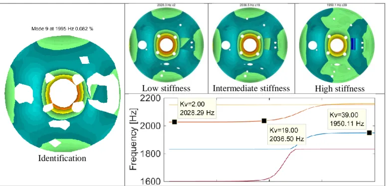
As a second illustration of mode crossing, test mode #9 where the main hole is deforming a lot (see Figure 18) had an initial MAC value of 77% (full contact surface, mode at 1950Hz). Within the range of contact stiffness, the results can be very significantly improved with intermediate (leading to a MAC above 90%) or low contact stiffness.
A non-trivial trend is that the frequency of this mode decreases for a high contact stiffness as shown in Figure 18 bottom right. For low stiffness, the cable guide mode is below in
frequency and thus for the considered plate mode has an out of phase cable guide contribution. This leads to a lower apparent mass and thus a higher frequency. For high stiffness, the cable guide mode moves in phase and the frequency is lower. As expected, until the cable guide mode frequency comes above the test frequency of the plate mode, the
frequency does increase with contact stiffness. It is the crossing that leads to the frequency drop.
Identification
Low stiffness Intermediate stiffness High stiffness
Figure 18 : Identified modeshape (left), Modeshape evolution with stiffness (top right) and Frequency evolution with stiffness (bottom right).
CONCLUSION
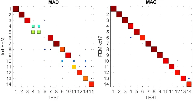
The paper illustrated the correlation and model updating processes used at CBI. The use of exact geometries was first shown to be critical particularly at higher frequencies. For material properties, it was shown that updating without first correcting the geometry leads to bias in the estimated properties. Finally for assemblies, modeshape correlation is typically needed and unknowns in the contact properties can lead to very significant variations of modal properties. Strategies to handle the unknown contact surface were proposed and proved to be very efficient for the considered test case.
Figure 19 : Initial MAC (left) and MAC with the updated FEM in geometry, material properties and contacts (right)
REFERENCES
(1) LAUWAGIE, T., VAN HOLLEBEKE, F., PLUYMERS, B., et al, “The impact of high-fidelity model geometry on test-analysis correlation and FE model updating results”, Proceedings of the international seminar on modal analysis, 2010.
(2) BALMES, E., et al, “Orthogonal Maximum Sequence Sensor Placements Algorithms for modal tests, expansion and visibility”, January, 2005, vol. 145, p. 146.
(3) MARTIN, G., BALMES, E., CHANCELIER, T., “Improved Modal Assurance Criterion using a quantification of identification errors per mode/sensor”, Proceedings of the international seminar on modal analysis, 2014.
(4) RUSINKIEWICZ, S., LEVOY, M., “Efficient variants of the ICP algorithm”, Proceedings. Third International Conference on IEEE, 2001, pp. 145-152.
(5) LOW, K.-L.. Chapel H., “Linear least-squares optimization for point-to-plane icp surface registration”, University of North Carolina, 2004.
(6) Vermot-Des-Roches, G., Rejdych, G., Balmes, E., Chancelier, T. , “The component mode tuning (CMT) method, a strategy adapted to the design of assemblies applied to industrial brake squeal”, Proceedings of EuroBrake, 2014.