Statistical identification of geometric parameters for high speed train catenary

Science Arts & Métiers (SAM)

is an open access repository that collects the work of Arts et Métiers Institute of Technology researchers and makes it freely available over the web where possible.

This is an author-deposited version published in: https://sam.ensam.eu

Handle ID: .http://hdl.handle.net/10985/8596

To cite this version :

Olivier VO VAN, Etienne BALMES, Jean-Pierre MASSAT - Statistical identication of geometric parameters for high speed train catenary - In: International Conference on Noise and Vibration Engineering, Belgium, 2014-09-15 - Proceedings ISMA - 2014

Any correspondence concerning this service should be sent to the repository Administrator : [email protected]

Statistical identification of geometric parameters for high

speed train catenary

O. Vo Van1,2, E. Balmes2,3, J.-P. Massat1

1

SNCF research department,

40 Avenue des Terroirs de France, 75611 Paris Cedex 12, France e-mail: olivier.vo [email protected]

2

Arts & Metiers ParisTech, PIMM

157 boulevard de l’hopital, 75013 Paris, France

3

SDTools

44 rue Vergniaud, 75013 Paris, France

Abstract

Pantograph/catenary interaction is known to be strongly dependent on the static geometry of the catenary, this research thus seeks to build a statistical model of this geometry. Sensitivity analyses provide a selection of relevant parameters affecting the geometry. After correction for the dynamic nature of the measurement, pro-vide a database of measurements. One then seeks to solve the statistical inverse problem using the maximum entropy principle and the maximum likelihood method. Two methods of multivariate density estimations are presented, the Gaussian kernel density estimation method and the Gaussian parametric method. The results provide statistical information on the significant parameters and show that the messenger wire tension of the catenary hides sources of variability that are not yet taken into account in the model.

1

Introduction

Development of numerical models is a main focus of current research in pantograph-catenary interaction. As shown in the benchmark led by S. Bruni [1], software modeling this interaction are becoming very accurate. Simultaneous improvement of simulation speeds makes the use of parametric or statistical studies possible. An important trend of studies performed at SNCF is to introduce variability into the deterministic parameters in order to make the model more robust to the high variability of experimental conditions. Moreover, a statistical approach is envisioned to allow revised maintenance policies which are known to usually be too restrictive on the controlled parameters.

A study by RTRI [2] analyzed the static geometry of the contact wire and showed, as our study [3], that the catenary geometry had a significant influence on current collection quality. The RTRI study highlights the criteria on the geometry most relevant to identify installation error. This gives information on the kinds of irregularities which significantly impact current collection quality, but does not give indications on which part of the catenary is the source of these irregularities.

The current paper seeks to solve the inverse problem. From a set of measured contact wire heights, one seeks to identify the probability distribution of influent parameters. After identifying sensitive parameters that will be considered as random and correcting measurements to provide a reference database for statistics, the method to solve the inverse stochastic problem is exposed. The last section analyses the results.

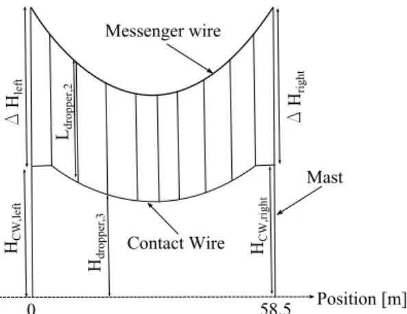
D H left Ldr oppe r,2 Hdr oppe r,3 Position [m] 0 58.5 Messenger wire Contact Wire Mast D H right HCW ,left HCW ,right

Figure 1: Parameters defining static geometry of a span

2

Case study

A catenary is divided into sections of about 1 km long. But every section is different. The largest standard structure of a catenary is thus a span, which for which one will seek to generate a statistical description. The two most used types of spans in the French catenaries for high speed trains are of 58.5m and 54m long, respectively named N2 and N3 (N for nominal). N2 is used for statistics of this paper, leaving the N3 for future verifications of conclusions.

One will first perform a sensitivity analysis to select random parameters and clarify the procedure used to obtain reference data from measurements.

2.1 Sensitivity analysis

Figure 1 illustrates the different parameters that can control the static geometry of the catenary (only tension and gravity are applied). These parameters are described below:

• HCW,lef tandHCW,rightare the height of the contact wire respectively at the left and right steady arm

of the span

• Hdrop,iis the height of the contact wire under theithdropper of the span

• ∆Hlef tand∆Hrightare the distance between the contact wire and the messenger wire respectively at

the left and right mast of the span

• Ldrop,iis the length of theithdropper of the span

• TCW andTM W are respectively the tensions in the contact wire (CW ) and in the messenger wire

(M W )

• The bending stiffness is negligible compared to the tensions applied in both cables and quick

para-metric studies have shown that a very large variation is needed to be able to see a variation on static deflection.

Figure 2 shows the impact of a variation of ±20% on the contact wire height. One observes that the variation ofTCW has a negligible impact compared to that created by the variation ofTM W. This is expected since

the conducting wire is mostly flat, while the messenger curvature is needed for to support the weight. In the light of this result,TCW can be removed from the list of stochastic parameters.

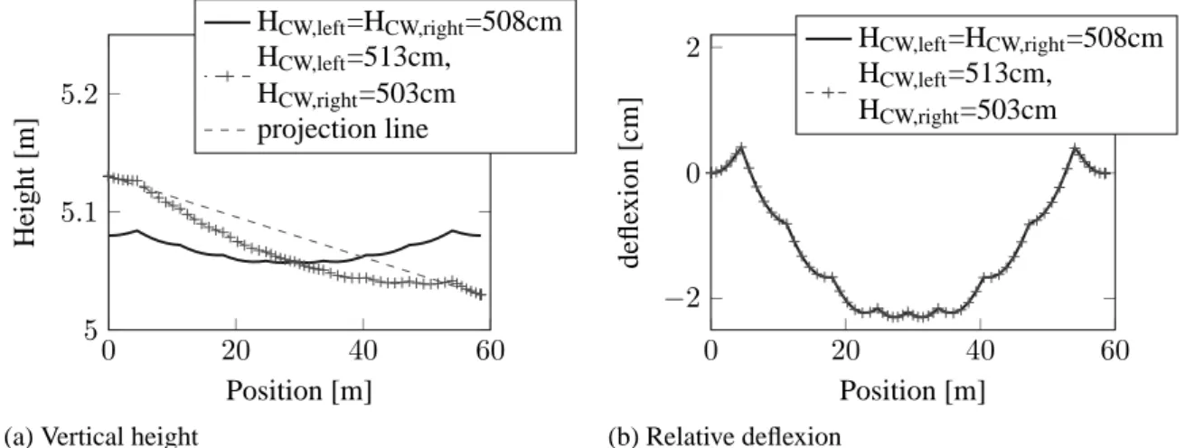
Figure 3a shows the contact wire height in two conditions. The nominal case withHCW,right= HCW,lef t= 508cm and a second configuration where the left mast has been raised of 5cm, while retaining the contact

0 20 40 60 5 5.05 5.1 5.15 5.2 Position [m] H eig h t [m] TCW=20800 TCW=26000 TCW=31200

(a) Contact wire

0 20 40 60 5 5.05 5.1 5.15 5.2 Position [m] H eig h t [m] TMW=16000 TMW=20000 TMW=24000 (b) Messenger wire

Figure 2: Variation of ±20% in TCW (left) and inTM W (right)

wire and the messenger wire is distance of140cm, and similarly the right mast has been lowered by 5cm in

order to amplify the potential variation of the deflection. The deflection after projection on the line linking the two steady arms, shown in 3b, is nearly identical in both cases. One can thus clearly say thatHCW,right

andHCW,lef thave no influence onCW deflection if ∆Hright and∆Hlef t do not change. Consequently,

these parameters will not be taken into account in the following.

0 20 40 60 5 5.1 5.2 Position [m] H eig h t [m] HCW,left=HCW,right=508cm HCW,left=513cm, HCW,right=503cm projection line

(a) Vertical height

0 20 40 60 −2 0 2 Position [m] d efl ex io n [c m] HCW,left=HCW,right=508cm HCW,left=513cm, HCW,right=503cm (b) Relative deflexion

Figure 3: Variation of+5cm for HCW,lef tand −5cm for HCW,right

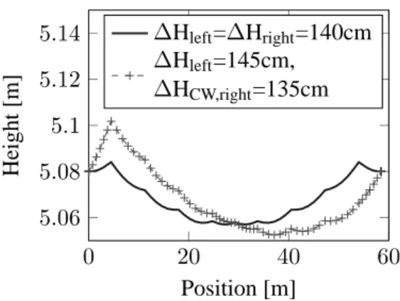
Finally figure 4 shows that∆H impacts the sag in a non-symmetric way. This parameter is thus retained.

After sensitivity analysis,11 parameters are retained and assumed independent: the 9 dropper lengths Ldrop,i,

the messenger wire tensionTM W and the distance between the contact wire and the messenger wire at the

mast∆H.

2.2 Available measurements

The measurements used were obtained on the catenary between Paris and Strasbourg (LN6). The measuring equipment is a pantograph keeping contact with the contact wire by applying a vertical force on it of approx-imately36N . The pantograph is fixed on a 40km/h moving train. These experimental conditions appeared

to have a significant impact on the measured sag. The data were thus corrected through an iterative scheme before which one built the model of each catenary on which the measure is complete, with the exact stagger and distances between spans. The nominal height is then defined by using dropper tables [4] and fixing

0 20 40 60 5.06 5.08 5.1 5.12 5.14 Position [m] H eig h t [m] ∆Hleft=∆Hright=140cm ∆Hleft=145cm, ∆HCW,right=135cm

Figure 4: Variation of+5cm for ∆Hlef tand −5cm for ∆Hright

contact wire height at steady arm to 5.08m and height of contact wire at masts 1.4m above. The process

applied is follows the steps shown in figure 5.

Reference sag

Static sag at iteration n

Dynamic simulation

36N and 40km/h

Uplift under pantograph (simulation of measure)

±

Real uplift

from measurement Gap

Hdrop,n+1 = Hdrop,n + Gap Inverse static Stop - + pP Gap2 > 1mm pP Gap2 _{< 1mm}

Figure 5: Parameters defining static geometry of a span 2

One first computes the static sag of the nominal catenary model, then runs a dynamic simulation correspond-ing to the measurement conditions, that is to say a pantograph applycorrespond-ing a36N mean-force on a train going at 40km/h. From this dynamic simulation, one can get the uplift under the pantograph. This value is what the

equipment assumes to be the static sag, but should more appropriately be called dynamic sag. The difference between the measured and simulated dynamic sags then gives an estimate of the geometry error. This gap is assumed to be representative of the error on the static sag, so that one seeks to correct the static geometry accordingly.

Obtaining a geometry that matches the target sag is an inverse static problem. The method applied here is to let only dropper lengths vary. This leads to a well posed problem that has a unique solution. The updated geometry can then be used at stepn + 1.

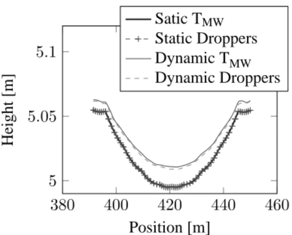
380 400 420 440 460 5 5.05 5.1 Position [m] H eig h t [m] Satic TMW Static Droppers Dynamic T_MW Dynamic Droppers

Figure 6: Comparison of impact ofTM W andLdrop,ion the dynamic correction applied

convergence is observed after2 iterations with a normpP Gap2 _{< 1mm.}

While using this method, two assumptions are made

• The bias corrected is significantly higher than the remaining measurement uncertainty and the model

uncertainty,

• The correction made only with dropper length variation leads to an equivalent solution as the one

which would have been found with the combination of all variations.

This second assumption can be verified by comparing the dynamic sag of two similar static sag obtained by different ways. While settingTM W to16kN for one model, one build another model with the same sag

with TM W = 20kN by modifying dropper lengths only. The figure 6 shows that the difference is lower

than2mm which is the order of magnitude of the measure resolution. Besides, one sees how important the

correction is by comparing the dynamic and static sag. This observation thus strengthens the first hypothesis too.

For the database of measurements, a set of 117 N2-span deflections were obtained. Each had different heights at masts but as seen in seen in section 2.1, height of the contact wire at mast has no impact on the deflection. In order to remove these parameters from measurements, projections are done as in figure 3.

The reference data is thus a set ofνexp = 117 experimental observations (Wobs,expi )1_<=i<=ν

exp considered as independent realizations of a random vector(Wobs,exp_i ) of size 9.

3

Methods for stochastic inverse problem solving

In this section, one defines the methods chosen to solve the stochastic inverse problem. The global framework used is explained in [5] and follows the steps detailed here.

The input parameters chosen in 2.1 are assembled in a random vector X defined in (1). Each of them is

supposed an independent random scalar.

X = [(Ldrop,i)1_<=i<=9, T_{M W}, ∆H] (1)

One first defines a parametric distribution for each element ofX following the maximum entropy principle

and tensions cannot be negative. The maximum entropy method thus leads to the same gamma distribution whose probability density function (p.d.f.) is given by

pX(x) = xk−1_{exp (−x/θ)} θk_Γ(k) (2) with Γ(k) = Z ∞ 0 e−x xk−1dx (3)

In order to get more readable results and a good conditioning, these p.d.f. are characterized by their expec-tations and standard deviations:

µ = kθ and σ =√kθ2

(4) One then callss the vector of hyper-parameters, gathering together the µiandσiof each scalarXifromX. s is a 24-length vector whose initial value s0 is set consistently with measurement magnitudes. This value

enables to get samples ofX of size Nigenerated by a specific sampling method, which is used to compute

the deflection of the contact wire.

LetWobs_{be the output random vector defined by thed}

Wobs = 9 non independent heights of the contact wire under droppers.

Four sample draws Xi,1<=i<=4 of X of size N1 = 103, N2 = 104, N3 = 105 and N4 = 106

were generated. As all marginal input distributions are supposed independent, the sampling method chosen is the Latin Hypercube Sampling method (LHS). Once the 4 corresponding samplesWobs_i computed, the distribution ofWobsis estimated using two different methods:

• Parametric estimation : one uses a gaussian distribution in order to represent the random vector Wobs. This method displays a quick1/√N convergence but can introduce a bias if the parametric

distribu-tion chosen is not fitted

• Non-parametric estimation: one uses the multivariate gaussian kernel density estimation method (called

KS for Kernel Smoothing). This method is slower with aN−1/(dW obs+4) convergence but does not introduce any bias.

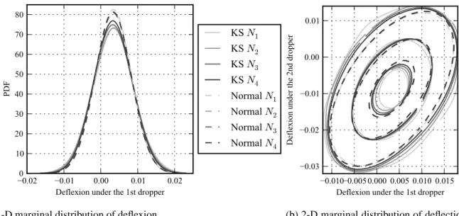
The theoretical convergence speed of the two methods is significantly different. For example, if one supposes a mean deflection under the 5th dropper of -2.5cm with a standard deviation of 1cm (approximately the mag-nitude observed), the estimation of the mean with a sample of size 1000 will have 95% of probability to be in the interval_{[−2.438cm, −2.562cm] with the parametric estimation method and [−1.348cm, −3.652cm]} with the non-parametric estimation method. One thus wants to check if the bias introduced is important. To this end, figure 7 compares the two methods for thei samples computed. On both figures, one sees that solid

lines (i.e. non-parametric estimation) get closer to the dashed lines (i.e. parametric estimation), which seems to have already converged with a 1000-sized sample. Moreover, usings0 as initial hyper-parameters, the

output samples all succeed in the Henze-Zirkler’s multivariate normality test. One thus chooses to use the parametric estimation method and verify if the result does still succeeds the normality test.

Callingpprior

Wobs, the estimation of the output distributionWobswith selected hyper-parameterss, one com-putes the likelihood

J (s) = ln(pprior_Wobs(W

obs,exp

1 ; s) + ... + ln(pprior_Wobs(W

obs,exp

νexp ; s). (5)

The maximum likelihood principle is an optimization problem given by

sopt = arg max J (s) (6)

In the implementation, the optimization is solved with the Nelder-Mead simplex algorithm available in the

−0.02 −0.01 0.00 0.01 0.02 Deflexion under the 1st dropper 0 10 20 30 40 50 60 70 80 PD F

KS

KS

KS

KS

Normal

Normal

Normal

Normal

(a) 1-D marginal distribution of deflexion

under the1st_dropper

−0.010−0.0050.000 0.005 0.010 0.015 Deflexion under the 1st dropper −0.03 −0.02 −0.01 0.00 0.01 D efl exi on unde r t he 2nd droppe r

(b) 2-D marginal distribution of deflection

under the1st_and2nd_droppers.

Iso-contours at level 100, 1000 and 3000

Figure 7: Comparison between parametric (dashed) and non-parametric (solid) estimation methods for sam-ples of sizesNi

To summarize, one choses 11 independent gamma distributions for input parameters, which creates a vector

of hyper-parameters to be defined. One uses the LHS method to compute a sample of Wobs which is estimated by a Gaussian multivariate parametric method in order findsoptwhich maximizes the likelihood ofpprior

Wobsregarding theνexpexperimental observations(W

obs,exp

i ).

4

Results

The statistical identification was motivated by the observation of the results obtained by the variation of dropper lengths only. The first part of this section thus shows these observations and their limits, the next analyses the final identification results.

4.1 Droppers only

When maintaining fixed every parameters but the dropper lengths, the inverse problem is well posed as explained in section 2.2. The problem is thus quick to solve and results are obtained in a few minutes. The 117(Wobs,exp_i ) thus lead to 117 sets of Ldrop,ion which statistical observation can be performed.

Table 1: Dropper length moments

H H H H H s X

Ldrop,1 Ldrop,2 Ldrop,3 Ldrop,4 Ldrop,5 Ldrop,6 Ldrop,7 Ldrop,8 Ldrop,9 µ − Lnom[cm] 0.64 -0.45 -0.68 -0.6 -0.34 -0.36 -0.08 0.19 0.95

σ[cm] 0.33 0.81 1.43 1.83 1.83 1.81 1.50 0.98 0.41

Table 1 shows that the expectation of dropper lengths is higher than the nominal value at the extremities and lower in the center of the span with a gap of almost1cm for some cases. Moreover, the standard deviation

is very high at the center of the span and low at extremities.

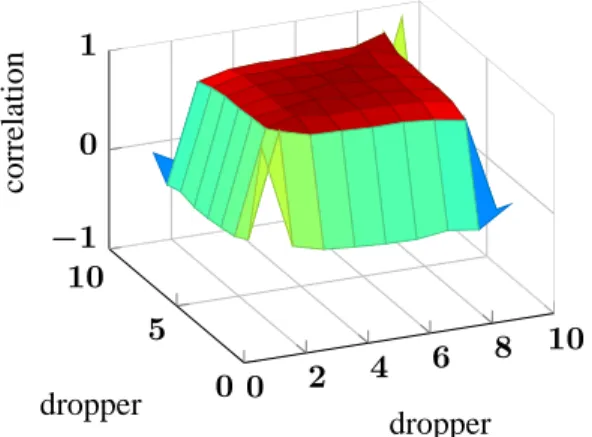
Figure 8 displays the Pearson matrix correlation which shows a very strong correlation of almost 1 between every droppers but those at the extremities. The high disparity of dropper lengths, the high gap between

0 2 4 6 8 10 0 5 10 −1 0 1 dropper dropper co rr ela tio n

Figure 8: Pearson correlation matrix of dropper lengths

nominal length and expectations obtained, and the strong correlation between dropper lengths leads to the conclusion that other parameters not taken into account have a non-negligible variability, which impacts the contact wire deflection.

4.2 Statistical identification

Taking parameters discussed in section 2.1, the whole inverse stochastic problem is solved under python with OpenTURNS [7] module while the static problem is solved by OSCAR[8] parallelized on 40 nodes. Each single static computation lasts around 2s, which leads to an evaluation of J (s) in around 80s. One

converged to the result after 2300 iterations with 3300 evaluations ofJ (s) in 3 days.

A first optimization led to high mean values of dropper lengthsLdrop,icompensated by a high mean value

ofTM W. These incoherent results have been solved by fixing the mean values ofLdrop,i which are the

only measured quantity during maintenance and consequently the most relevant quantity to maintain fixed. The resultingsoptis displayed in Table 2

Table 2: Optimal statistical parameterssopt

H H H H H s X

TM W ∆H Ldrop,1 Ldrop,2 Ldrop,3 Ldrop,4 Ldrop,5 Ldrop,6 Ldrop,7 Ldrop,8 Ldrop,9 µ[SI] 20575 1.388 1.244 1.098 0.998 0.945 0.934 0.945 0.998 1.098 1.244

σ[SI] 818 0.0065 0.0067 0.0050 0.0045 0.0045 0.0038 0.0044 0.0035 0.0034 0.0070

Table 2 shows thatTM W has a standard deviation of around 818N, which is a very large value since this

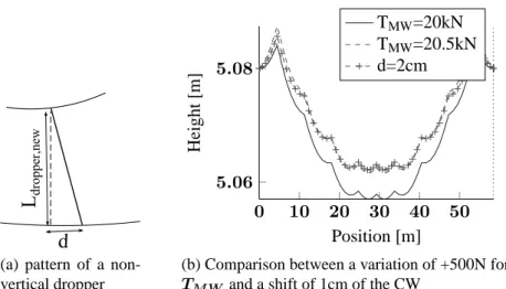
tension is regulated by masses installed at the forward and after ends of the catenary. One thus has to investi-gate the reason of this large variation, which can be observed in a single catenary. An possible explanation is the global shifting of the contact wire relatively to the messenger wire due to the creep or thermal expansion. Figure 9 shows that a shifting of 2cm can induce a variation of deflection as high as an increase of 500N of

TM W.

While in the model taken, heights of the contact wire at the steady arms have been fixed in order to get the chosen∆H, the real height is variable, but depends on several parameters. For example, the dropper lengths

of droppers close to the steady arm and the lengths of the two spans linked by the steady arm seem to have a significant influence. ∆H is thus not independent of some Ldrop,ias one has supposed before. The model

could thus be improved taking into account this information.

During the manufacturing of droppers, the measurement accuracy on their length is1cm. The Ldrop,ifound

L

oppe

r,new

d

(a) pattern of a non-vertical dropper 0 10 20 30 40 50 5.06 5.08 Position [m] H eig h t [m] TMW=20kN TMW=20.5kN d=2cm

(b) Comparison between a variation of +500N for

TM W and a shift of 1cm of the CW

Figure 9: Impact of a shift of the CW on the deflection

0 20 40 60 −6 −4 −2 0 2 ·10−2 Position [m] D efl ex io n

[m] Confidence region associated

with probability level 0.98

Wexp,obs

Mean computational model

Figure 10: Deflection of the contact wire at dropper positions along the span

twice higher variation around the extremities of the span. This issue can be due to the link with∆H not taken

into account or to a bias induced by either measurement or model which have been mixed while correcting measurements.

Figure 10 shows the confidence region in which the deflection has a98% of probability to be, considering

the input gamma distributions chosen with hyper-parameterssopt. One observes a large area which is mainly due to the method applied to maximize uncertainty (maximum entropy principle).

5

Conclusion

This paper illustrated the possibility to use statistical inverse problems to characterize the distribution of catenary geometries based on a few sensitive parameters. While the method was eventually found to be quite efficient, the initial analysis ignored the key parameter of messenger wire tension and led to inconsistent results. This highlights the importance of initial parameter choice and the presence of strong bias when this choice is not properly made.

In the end, it appears global shifting of the contact wire relatively to the messenger would have an impact similar to that of variations in the tension and that one should not ignore the correlation of certain parameters like wire distance at mast and nearby dropper lengths.

method to estimate the posterior probability distribution frompprior,opt_Wobs = p

prior

Wobs(sopt) [9, 5].

In the near future, this statistical geometric model will be used to generate random geometries and use them as input for dynamic simulations, thus resulting in statistics on the pantograph contact force, which is the key parameter of interest. Adjusting maintenance rules will be possible if a clear relation between statistics on geometry and contact force can be obtained.

References

[1] S. Bruni et al. “The pantograph-catenary interaction benchmark”. In: Proceeding of the 23rd

Interna-tional Association for Vehicle System Dynamics Symposium (2013). Ed. by Z. Shen.

[2] M. Aboshi and M. Tsunemoto. “Installation Guidelines for Shinkansen High Speed Overhead Contact Lines”. In: QR of RTRI 52.4 (2011), pp. 230–236.

[3] O. Vo Van, J.-P. Massat, and E. Balmes. “Introduction of variability into pantograph-catenary dynamic simulations”. In: Proceeding of the 23rd International Association for Vehicle System Dynamics

Sym-posium (2013). Ed. by Z. Shen.

[4] IGTE. Dropper table for normal and special spans. Tech. rep. 21411/310545. SNCF, 2010.

[5] C. Soize. “Stochastic modeling of uncertainties in computational structural dynamics - Recent theoret-ical advances”. In: Journal of Sound and Vibration 332.10 (2013), pp. 2379–2395.

[6] E. T. Jaynes. “Information theory and statistical mechanics. II”. In: The Physical Review 108.2 (1957), pp. 171–190.

[7] EDF, EADS, and PhiMeca. Reference Guide Open TURNS version 1.1. Tech. rep. EDF EADS -PhiMeca, 2013.

[8] E. Balmes, J.-P. Bianchi, and J.-P. Massat. OSCAR 1.0 user’s guide. Tech. rep. SNCF and SDTools, 2011.

[9] J. L. Beck and L. S. Katafygiotis. “Updating models and their uncertainties. I: Bayesian statistical framework”. In: Journal of Engineering Mechanics 124.4 (1998), pp. 455–461.