Science Arts & Métiers (SAM)
is an open access repository that collects the work of Arts et Métiers Institute of
Technology researchers and makes it freely available over the web where possible.
This is an author-deposited version published in: https://sam.ensam.eu Handle ID: .http://hdl.handle.net/10985/16559
To cite this version :
Bessam ZERAMDINI, Camille ROBERT, Guénaël GERMAIN, Thomas POTTIER - Numerical simulation of metal forming processes with 3D adaptive Remeshing strategy based on a posteriori error estimation - International Journal of Material Forming - Vol. 12, n°3, p.411-428 - 2018
Any correspondence concerning this service should be sent to the repository Administrator : [email protected]
1
Numerical Simulation of Metal Forming Processes with 3D Adaptive Remeshing strategy
based On A Posteriori Error Estimation in Large Deformation Finite Element Analysis
Bessam Zeramdini
1, a), Camille Robert
1, b), Guenael Germain
1, c)and Thomas Pottier
2, d)1LAMPA, Arts et Métiers ParisTech at Angers
2 Boulevard du Ronceray, BP 93525, F-49035 Angers cedex 01, France 49100 Angers
2Ecole Nationale Supérieure des Mines d’Albi
Mines d’Albi-Carmaux, Campus Jarlard 81013 Albi
Abstract. In this work, a fully automated adaptive remeshing strategy, based on a tetrahedral element for 3D metal
forming processes, was proposed in order to solve large deformation problems associated with the severe mesh distortion that occurs during the computation. The main idea is to use the h-type adaptive mesh in combination with an a-posteriori error estimator measured (by the energy norm) on each mesh elements to locally control the mesh modification-as-needed. Once a new mesh is generated, all history-dependent variables must be carefully transferred between subsequent meshes. Therefore, several transfer techniques are described and compared; and special attention is given to restore the local mechanical equilibrium of the system. Finally, after presenting the necessary adaptive remeshing steps, some 3D analytic and numerical results using the proposed adaptive strategy are given to demonstrate the capabilities of the equilibrated approach and to illustrate some practical characteristics of our remeshing process.
Keywords. 3D metal forming processes, Automatic adaptive remeshing, A-posteriori error estimator, Transfer
techniques, Equilibrated process
1 INTRODUCTION
For a large class of problems such as metal forming process like forging, rolling, cutting, etc., the use of the finite element method is still a challenging problem. It can typically involve high strain localization, large inelastic deformations and high temperature problems. Often in these types of application, mesh becomes unacceptable due to severe distortion or complex workpiece-die contact occurring which induces errors in the key internal variables (plastic strains and stresses) [Hamel 00]. As consequence, the ability to achieve a proper analysis with reasonable CPU cost is entirely dependent on the FE mesh spacing. Indeed, optimal mesh configuration changes continuously throughout the metal forming process. Consequently, the final results obtained with the use of a fixed mesh are unreliable and may give a rise to severe numerical difficulties and may even make it impossible to pursue the calculations any further because of severe element distortion. In order to overcome these difficulties and continue the simulation for large deformation cases, successive mesh adaptation is needed during the numerical simulation in order to obtain an optimal discretization according to the geometrical shape or/and physical solution. The main ingredients in any adaptive procedure are a posteriori error estimation and a mesh generator [Diez 07]:
(i) The a posteriori error estimation is required to decide if the previous FEM calculation must be stopped, to locate the critical zones of the domain where the new elements need to be concentrated or to be coarsened and to
2
determine the size of optimal mesh. An overview of different a posteriori error estimation technique is provided
by [Ainsworth 97, Verfurth 99].
(ii) The mesh generator produces the new spatial discretization with the desired element density at prescribed locations in the deformed configuration, as determined after the error assessment. While the spatial discretization changes between subsequent mesh, the global topology of the piece is conserved. In the approach presented here, unstructured tetrahedral elements with local h-adaptive strategy guided by error indicators and geometric approximation are used. The advantages of their use are discussed by Lo [Lo 91, 91a].
Once a new mesh is generated, two approaches are possible: either the simulation is totally recomputed, or all the state variables and history-dependent variables at the end of the previous load step must be transferred from the degenerated old mesh to the reconstructed new one, in order to continue the simulation. Owing to the fact that the optimal mesh configuration and the boundary conditions changes continuously throughout the numerical simulation, the second approach will be implemented step by step in order to adapt to this change. This is a delicate issue because if the new field variables are not adequately determined, the simulation accuracy can be severely affected
[Dureisseix 06]. Different techniques exist to transfer the history variables; basically all these methods can be
categorized into two types: direct transfer (weighted average method [Habraken 90], diffuse approximation method
[Hamel 00], closest point technique [Srikanth 00], etc ) and indirect transfer (such as least squares smoothing, average
values [Peric 96], the superconvergent patch recovery (SPR) technique [Zienkiewicz 92],etc ).
In the present paper, after a concise review of error estimation and the alternative mesh refinement criteria in Section 2, different Patch Recovery Techniques such as average values technique (Avg), superconvergent patch recovery (SPR) and the modified of Zienkiewicz and Zhu technique (SPR-P) will be described in Section 3. Then in Section 4 these recovery methods will be compared with analytics function in order to select the best techniques to transfer the data state variables between two successive meshes. In Section 5, the global flowchart of the proposed 3D adaptive remeshing algorithm is detailed. In Section 6, the efficiency of algorithm here proposed and the equilibrated approach are validated through various examples including the shear test as well as the forging process. Finally some conclusions are drawn in Section 7.
2 ERROR ESTIMATORS
The error estimation is the first and one of the most important procedures in adaptive FE analysis. Because it’s indicates the quality of elements, quality of the solution, and if necessary new element density. Among the very numerous proposals that were, and still are available, three groups can be classified, depending on whether they are based on: the estimators based on residuals analysis, introduced by Babuska and Rheiboldt [Babuška 78], the estimators based on the concept of error in constitutive relation, initiated by Ladvéze et al. [Ladevèze 86], and the estimators based on smoothing techniques developed by Zienkiewicz et Zhu [Zienkiewicz 87].Although the approach of the residual estimator proposed by Babuška and Rheinbold [Babuška 78] is mathematically rigorous, its extension to 3D nonlinear problems is facing some major challenges. Indeed the efficiency of this estimator depends on the mesh quality and regularity of the solution, which makes it less suitable for large deformation problems. In the literature, the majority of applications are presented in the context of 1D and 2D academic problems. The key point of the proposed estimator by Ladevèze et al. [Ladevèze 86] is the construction of admissible displacement-stress pair. For the sake of simplicity, in the context of FE method with compressible material, the displacement field can be considered as admissible. Conversely, the stress field is not statically admissible. In the literature, Sever method can be used to calculate this admissible stress [Fraeijs 65, Ladevèze 97]. In spite of its remarkable efficiency, this technique has been rarely used in FE simulation software because of the cost of its implementation. In this work, the estimator based on smoothing techniques is used due to its cost effectiveness and reliability to estimate errors and for its simplicity of implementation. The main idea of the smoothing techniques is based on the construction of a recovered stress tensor field σ̃, more accurate than the finite element solution σh. This recovered stress tensor field σ̃, can be constructed by
3
a variety of projection techniques, such as: least squares smoothing, average values and the superconvergent patch recovery (SPR) technique.
In the following part, the average values technique, the SPR error estimator in its almost standard form and the modified Zienkiewicz and Zhu technique (SPR-P), will be studied.
2.1 A posteriori error estimation
We suppose that the FE solution (𝑢ℎ, 𝜎ℎ) is an approximation of the exact solution (𝑢, 𝜎) in the considered finite element space Ω. The displacement error 𝑒𝑢 is the difference between the exact displacement solution and the FE displacement solution:
𝑒𝑢= 𝑢 − 𝑢ℎ (1) The stress error 𝑒𝜎 is the difference between the exact stress field and the FE stress field:
𝑒𝜎= 𝜎 − 𝜎
ℎ (2) Dealing with problems of metal forming process and mechanical structure, the element error is generally given, according to the norm of energy [Boussetta 04, 06]. It expresses the difference between the exact stress σ and the FE ones 𝜎ℎ:
‖𝑒𝜎‖
𝑒𝑙= ‖𝜎 − 𝜎ℎ‖𝑒𝑙 = (∫(𝜎 − 𝜎ℎ) ∶ (𝜀 − 𝜀ℎ) 𝑑𝜔)1/2 (3) To evaluate the quality of the approximate error norm it is more logical to use a relative value, given as:
𝜃𝑒𝑙 = ‖𝑒𝜎‖𝑒𝑙
(∫ 𝜎:𝜀 𝑑𝜔Ω )1/2 (4) Practically, it is not possible to compute the exact error 𝑒𝜎. The exact solutions (𝜎, 𝜀) are further approximated by smoothed stress distribution ones (𝜎̃, 𝜀̃), which are computed from the FE solutions using Patch Recovery Techniques presented thereafter. Therefore, the stress error modelling is given by:
𝑒𝜎̃= 𝜎̃ − 𝜎ℎ (5) Dealing with problems of metal forming process and mechanical structure, the element error norm will be defined by:
‖𝑒𝜎̃‖
𝑒𝑙 = ‖𝜎̃ − 𝜎ℎ‖𝑒𝑙= (∫(𝜎̃ − 𝜎ℎ) ∶ (𝜀̃ − 𝜀ℎ) 𝑑𝜔)1/2 (6) Then, the global error 𝜃 ̃ over the whole structure Ω is calculated by summing the errors of all the elements.
‖𝑒𝜎̃‖2 Ω= ∑ ‖𝑒𝜎̃‖ 2 𝑒𝑙 𝑒𝑙∈Ω (7) 𝜃̃ = (∑ (𝜃̃𝑒𝑙)2 𝑒𝑙∈Ω ) 1/2 (8) 𝜃̃𝑒𝑙 = ‖𝑒𝜎̃‖ 𝑒𝑙 (∫ 𝜎̃:𝜀̃ 𝑑𝜔)1/2 (9)
The dependability of the estimate is measured by its effectivity index ξ defined, in each element of the mesh, as the ratio between the predicted error and the exact error as measured respectively in expression (6) and expression (3). Thus:
ξ =‖eσ̃‖el
‖eσ‖el (10) An error estimator is considered as asymptotically exact when its efficiency index tends to 1, in other words when the size of items tends to zero [Zienkiewicz 92b, Ainsworth 97, Boussetta 06].
4
2.2 Size map for adaptive strategies
After estimating the element error, an establishment of a relation between this error and the element size is needed afterwards. Usually, this relation can be established with the using either of the following two strategies: The first allows us to calculate an optimal mesh for a prescribed accuracy, while the second seeks to optimize a mesh under the constraint of a number of degrees of freedom attached. One may refer to [Boussetta 04, 06] for more details, which used a combination of them. The first strategy is used to compute an optimized new mesh. Then, if the number of elements exceeds the prescribed number of degrees of freedom the new mesh will be computed with the second strategy. Many others authors [Coorevits 04, Bellenger 05] propose other similar optimization strategies that aim to control the size of the problem studied. They seek maximum accuracy to reach for a fixed size memory or CPU time for a given calculation. In the present work, only the first strategy will be studied because the goal of this paper is to evenly distribute the error over all the elements.
Optimal mesh for prescribed accuracy
𝜃
𝑖𝑚𝑝According to finite element convergence theorem, the local element error is directly related to its characteristic length ℎ𝑒𝑙 and its rate of convergence 𝑝. In three-dimensional case, p is equal to 1 for the linear tetrahedron element
[Ciarlet 78].
𝜃̃𝑒𝑙 = 𝑂(ℎ𝑒𝑙𝑝) (11) Assuming that the rate of convergence of the FEM is uniform throughout the entire domain Ω, the optimal size of each element must be computed by:
𝜃̃ 𝑒𝑙opt 𝜃̃𝑒𝑙 = ( ℎ𝑒𝑙opt ℎ𝑒𝑙) 𝑝 (12) Where ℎ𝑒𝑙 and ℎ𝑒𝑙𝑜𝑝𝑡 denote respectively the current characteristic size of an element el and the optimal characteristic size of the new one. 𝜃̃𝑒𝑙 and 𝜃̃𝑒𝑙optrepresent the predicted and optimal element error to the current mesh and the optimal one, respectively.
𝜃̃ = (∑ (𝜃̃𝑒𝑙)2 𝑒𝑙∈Ω ) 1/2 (13) 𝜃𝑖𝑚𝑝= (∑ (𝜃̃ 𝑒𝑙𝑜𝑝𝑡)2 𝑒𝑙∈Ω ) 1/2 (14)
In three-dimensional case, the optimal number of elements is given by: 𝑛𝑒𝑙𝑡𝑜𝑝𝑡 = ∑ (ℎ𝑒𝑙𝑜𝑝𝑡 ℎ𝑒𝑙) −d 𝑛𝑒𝑙𝑡 𝑒𝑙 (15)
Where nelt is the total number of elements within the domain Ω and d is the number of degrees of freedom. The optimality condition of the expected mesh leads to uniform the error θuni on the new elements, which gives:
∀el , (θ̃elopt)2= (θuni)2(helopt
hel) −d
(16) From (equation14) and (equation 16), the target error θinp accepted by the user is given by:
(θinp)2= (θuni)2∑ (helopt
hel) −d nelt
el (17) Then, a new element size factor can be computed from (equation 12) and (equation 16)
5
helopt hel = ( θuni θ̃el) 2 2p+d (18) The final expression of the resize coefficient is written as a function of the estimated error, the target error and the convergence rate p: helopt hel=
(θinp)1/p (θ̃el) 2 2p+d(∑ (θ̃el)2p+d2d nelt el ) 1 2p(19)
3 PATCH RECOVERY TECHNIQUES
The transferring approach strongly depends on the kind of state variables which needs to be transferred [Khoei 07]. At least, when transferring the nodal variables (such as displacements, velocity and temperature) a direct interpolation from old nodes to the new ones may be used via the finite element shape function. However, the transfer of the element variables (such as stress, strain and internal variables) is a very difficult problem. This problem has been addressed by many authors [Hochard 95, Peric 96, Khoei 07].
Here, the nodal displacement data is already present in the updated geometry of the problem because the remeshing strategy is done in the deformed configuration. In fact, only integration point variables need to be transferred. It should also be noted that in the case of a thermo-dynamic test, also the temperature must be transferred from the old node to the new ones. In order to study the compatibility of the element state transfer with the initial field and the numerical diffusion solution, numerical result using three recovery methods will be compared in the next part with analytic and numerical problems.
3.1 Average values (Avg)
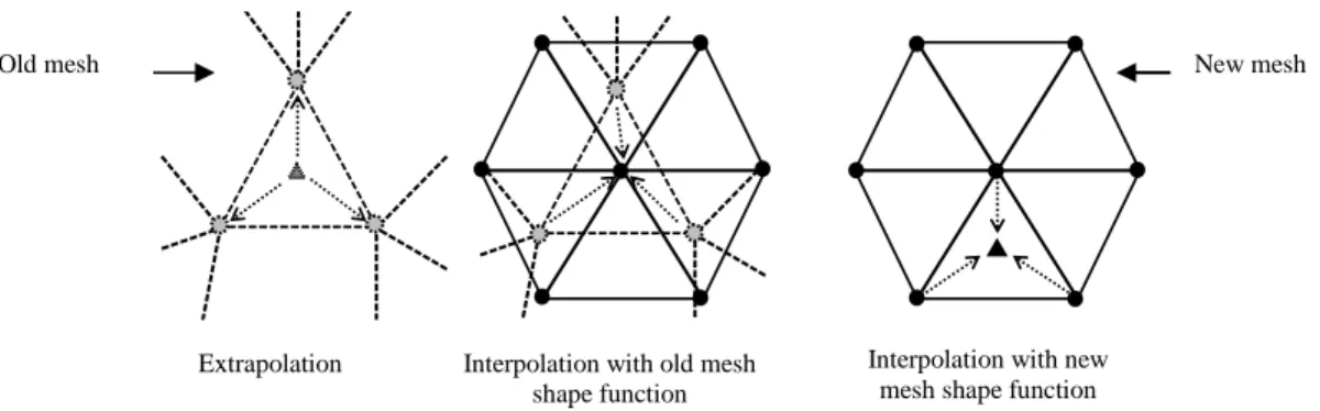
In each element patch Ωk, the Average values procedure for transferring element fields is splitted into three steps which are summarized in fig.1. First the average values are projected from the old Gauss point g to the old nodes k. Such that an element patch Ωk represents a union of elements containing the vertex node k (fig.3):
∀ k ∈ Ωoldk , σ̃k= 1 ∑ ∑g∈ elωg el∈ Ωoldk ∑ ∑ ωg g∈ el σe el∈ Ωoldk (20)
Where ωg and ωe are the volume contribution associated to Gauss point g and to element el, respectively.
Then, as mentioned in [zeramdini 16], the values at the new nodal points can be computed by simple interpolation of the old nodal values using the local interpolation functions such as the finite element shape function.
∀ k ∈ Ωold, σ̃x= ∑nntk∈ Ωold σ̃k Nold(ξ(x)) (21) Where nnt is the total number of node in each element, ξ(x) are the local coordinates of the new node x in the old mesh and Nold are the old FE shape functions used to interpolate the nodal variables.
Finally, the history dependent values at the integration points of the new mesh can be achieved by using local shape function of the new elements.
∀ x ∈ Ωnew, σ̃ = ∑nnt σ̃x Nnew
x∈ Ωnew (ξ(g)) (22) Where ξ(g) are the local coordinates of the new Gauss point in the new mesh and Nnew are the new FE shape functions.
6
Figure 1. A tree-step procedure illustrating the indirect element field transfer
This method has the advantage of being applicable easily to any type of complex three-dimensional case by not having to consider the discretization of the two meshes involved. But its first extrapolation step constitutes an important source of numerical diffusion. In order to limit this diffusion, many other advanced techniques have also been proposed such as the Super-convergent Patch Recovery proposed by Zienkiewicz et Zhu in 1992 [Zienkiewicz
92].
3.2 Super-convergent patch recovery (SPR) technique
The FE approximation of a one-dimensional linear function can be locally very different from the exact solution, as shown in Fig.2. However, at certain points in the elements, the results are nearly correct. These super-convergent points are located in the center of the elements witch correspond to the element Gauss points. This prediction is proposed by Zienkiewicz and Zhu [Zienkiewicz 92] and recommended by Babuska et al. [Babuška 94] through numerical investigations.
Figure 2. Approximated values and exact solution
To compute the recovered stress field σ̃ of each element (represented in equation 24), the following expression is generally used for each patch. Such that an element patch Ωk represents a union of elements containing the vertex node k (fig.3): ∀ k ∈ Ωoldk , σ̃ = ∑ σ̃ k nnt k=1 Nk(x, y, z) = ∑ P. ak Nk(x, y, z) nnt k=1 (23)
Figure 3. Two-dimensional superconvergent patch recovery (SPR)
Interpolation with new mesh shape function Interpolation with old mesh
shape function Extrapolation
7
The equation 23 is valid only over the old element patch Ωold, Where NG is the total number of Gauss points in the patch, N𝑘 are the FE shape functions used to interpolate the nodal variables, σ̃k is the recovered solution at node k computed by considering a polynomial expansion P and a is a vector of unknown parameters. For a three-dimensional problem and for linear tetrahedral elements, we have:
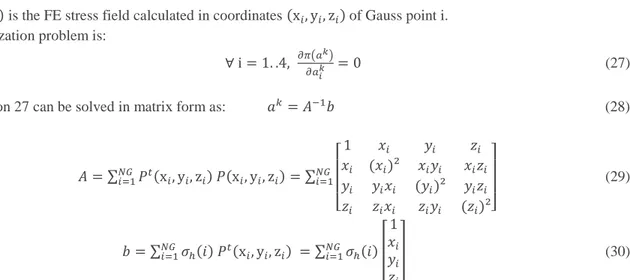
P = (1, x, y, z) (24) a𝑘= (a1𝑘, a2𝑘, a3𝑘, a4𝑘)𝑡 (25) The determination of the coefficients 𝑎𝑖𝑘 for each component of the stress tensor consists of minimizing the following functional: 𝜋(𝑎𝑘) = ∑ (𝜎 ℎ(𝑖) − σ̃ (𝑖)) 2 = ∑ (𝜎ℎ(𝑖) − P(x𝑖, y𝑖, z𝑖). ak N𝑘(x, y, z)) 2 𝑁𝐺 𝑖=1 𝑁𝐺 𝑖=1 (26)
Where 𝜎ℎ(𝑖) is the FE stress field calculated in coordinates (x𝑖, y𝑖, z𝑖) of Gauss point i. The minimization problem is:
∀ i = 1. .4, 𝜕𝜋(𝑎𝜕𝑎𝑘)
𝑖
𝑘 = 0 (27)
The equation 27 can be solved in matrix form as: 𝑎𝑘= 𝐴−1𝑏 (28) Where: 𝐴 = ∑𝑁𝐺𝑃𝑡(x𝑖, y𝑖, z𝑖) 𝑃(x𝑖, y𝑖, z𝑖) 𝑖=1 = ∑ [ 1 𝑥𝑖 𝑦𝑖 𝑧𝑖 𝑥𝑖 (𝑥𝑖)² 𝑥𝑖𝑦𝑖 𝑥𝑖𝑧𝑖 𝑦𝑖 𝑦𝑖𝑥𝑖 (𝑦𝑖)² 𝑦𝑖𝑧𝑖 𝑧𝑖 𝑧𝑖𝑥𝑖 𝑧𝑖𝑦𝑖 (𝑧𝑖)²] 𝑁𝐺 𝑖=1 (29) 𝑏 = ∑𝑁𝐺𝜎ℎ(𝑖) 𝑃𝑡(x𝑖, y𝑖, z𝑖) 𝑖=1 = ∑ 𝜎ℎ(𝑖) [ 1 𝑥𝑖 𝑦𝑖 𝑧𝑖 ] 𝑁𝐺 𝑖=1 (30) Finally, the elements smoothed stress distribution σ̃ is then computed at the node k (center of the patch) by inserting its coordinates in equations 23, where:
σ̃k= P(x𝑘, y𝑘, z𝑘) ak (31) The history dependent values at the integration points of the new mesh can be achieved by interpolating the obtained
nodal recovered solution σ̃k from old node to the new one using equations 21, then from old Gauss point to the new one using equations 22.
Figure 4. Recovery of 2D boundary nodes
Particularly, the superconvergent patch recovery (SPR) technique is often preferred by several authors because it is robust and simple to use [Boussetta 04, 06]. However, for borders nodes (Fig. 4), in the majority of cases the number of integration points is insufficient to determinate the coefficients of the polynomial expansion [Wiberg 94, Kumar 15]. In fact, the matrix A (equation 29) is non-reversible. For a border node, Zienkiewicz and Zhu [Zienkiewicz 92(a,b)]
8
propose to calculate the value of σ̃k from a topological patch centered on an internal node closest to extern node. Thus σ̃𝑘𝑒𝑥𝑡gets the neighbor value σ̃𝑘𝑖𝑛𝑡.
3.3 The Liszka-Orkisz variant of SPR (SPR-P)
In order to solve the boundary nodes problems the concept of the extended patch (see Fig. 5) introduced by Liszka-Orkisz’ and al.[Liszka 80, 84] can be used, where the nodal variables can be regarded as first (or second) order Taylor series expansion over the extended topology 𝑃 in the element patch Ωk. For linear constraints, a Taylor series expansion to the first order of the FE stress at the Gauss points can be given as:
∀ k ∈ Ωk, σ̃
k= P(xk, yk, zk) ak (32) (1st order) = a1k+ a2k(x − x
k) + ak3(y − yk) + a4k(z − zk) (33) Then, the minimization problem is:
𝜋𝑘𝐹𝐷(ak) = ∑ ( σg−(a1k+a2k(xg−xk)+a3k(yg−yk)+a4k(zg−zk))
∆𝑟𝑔2 ) 𝑔∈Ωk 2 = ∑ 𝑂((∆𝑟𝑔) 2 ) ∆𝑟𝑔4 𝑔∈Ωk (34) With: ∆𝑟𝑔2= (𝑥𝑔− 𝑥𝑘)2+ (𝑦𝑔− 𝑦𝑘)2+ (𝑧𝑔− 𝑧𝑘)2 (35) And similar to the standard form SPR the equation 34 can be solved in matrix form as: 𝑎𝑘 = 𝐴−1𝑏 (36) Where: 𝐴 = ∑ ∆𝑟1 𝑔4𝑃 𝑡(x 𝑔, y𝑔, z𝑔) 𝑃(x𝑔, y𝑔, z𝑔) 𝑁𝐺 𝑔=1 = ∑ ∆𝑟1 𝑔4 [ 1 ∆𝑥𝑔 ∆𝑦𝑔 ∆𝑧𝑔 ∆𝑥𝑔 (∆𝑥𝑔)² ∆𝑥𝑔∆𝑦𝑔 ∆𝑥𝑔∆𝑧𝑔 ∆𝑦𝑔 ∆𝑦𝑔∆𝑥𝑔 (∆𝑦𝑔)² ∆𝑦𝑔∆𝑧𝑔 ∆𝑧𝑔 ∆𝑧𝑔∆𝑥𝑔 ∆𝑧𝑔∆𝑦𝑔 (∆𝑧𝑔)² ] 𝑁𝐺 𝑔=1 (37) 𝑏 = ∑𝑁𝐺𝑔=1𝜎ℎ(𝑔) 𝑃𝑡(x𝑔, y𝑔, z𝑔) = ∑ 𝜎ℎ(𝑔) [ 1 ∆𝑥𝑔 ∆𝑦𝑔 ∆𝑧𝑔] 𝑁𝐺 𝑔=1 (38) With: ∆𝑥𝑔= 𝑥𝑔− 𝑥𝑘; ∆y𝑔= 𝑦𝑔− 𝑦𝑘 ; ∆z𝑔= 𝑧𝑔− 𝑧𝑘 (39) The weighting term ∆𝑟1
𝑔4 allows to varying the weight of the contributions of neighbors in the patch. This weight is
even important if the corresponding Gauss Point g is closer to the central node k of the patch. However in the SPR technique all the neighbors have the same weight.
9
4 ANALYTICAL RESULTS
4.1 Efficiency of the adaptive remeshing strategies
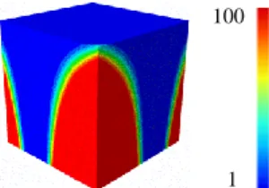
In this section, an analytical function f1(x, y, z)is used to check the sensitivity of the described a posteriori error estimation (section: Size map for adaptive strategies) for detecting the presence of significant error localization and to test the capabilities of the presented adaptive remeshing strategies (section: Patch Recovery Techniques) in the presence of various levels of pollution error.
f1(x, y, z) = 100 ∗ √tanh( 3(x − 0,3)7∗ (y − 0,3)7∗ (z − 1,3)5+ 1) (40) x: [−1. .1]
y: [−1. .1] z: [−1. .1]
Figure 6. The analytic values of the function 𝒇𝟏(𝒙, 𝒚, 𝒛)
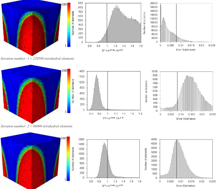
The adaptive procedure starts approximately with 21000 uniformly distributed elements. A target error in the adaptive process of 0.008% was adopted. The results are shown in Fig.7, where each row corresponds to a remeshing step taking the mesh in the previous row as the initial mesh. In practice, the elements size can’t respect perfectly the target error; hence, the sizes of elements can be very small or very large, especially in the high gradient zones. The main cause of this non respect is the obligation to insert a midcap mesh in these zones in order to create a better evolution of the mesh size map. To evaluate the efficiency of the different used processes, global and local checks can be used: a first check is undertaken to simply calculate the average error of the new discretization. If this error is not close to the desired precision, it is certain that the built mesh is not optimal. However, even if the overall error is close to the desired one, this does not prove the optimality of new mesh. The main idea of the local check is to verify the error of the entire domain Ω for each element. In fact, if the element size is optimal, the procedure of successive adaptation must give change coefficients close to 1. According to [Ladevèze 01], the size of the elements is considered satisfying in all areas where we have:
23 ≤ R𝑒≤ 3
2 , R𝑒 = hnew
hold (41)
As shown in fig.7, after each remeshing steps the density of element will increase or decrease in some zones in order to respect the target error. The evolution of the number of element in the histograms plot showed a concentration rise of elements numbers around the target error after each meshing step. For this analytic function four iterations
Initial mesh ≈ 20900 tetrahedral elements
100
1
100
10
Iteration number: 1 ≈ 229500 tetrahedral elements
Iteration number: 2 ≈ 86000 tetrahedral elements
Iteration number: 4 ≈ 10500 tetrahedral elements
Figure 7. Iso values of the tested analytical function 𝒇𝟏(𝒙, 𝒚, 𝒛), mesh size coefficient 𝑹𝒆, and local error estimation for each
remeshing step
can be considered as satisfactory because the modification coefficients of element size is 90%, close to 1 in overall domain. In thereafter examples this coefficients of element size criteria will be used in order to define the ideal number of iteration for each FEM problem.
4.2 Selection of the best Recovery Techniques
In order to select the best Patch Recovery Techniques to transfer the data state variables between two meshes, several analytical functions (linear and nonlinear) are considered (Table1). Here, we measure the exact error value, since the true solution is known. The approximated solution is made by using the smoothing techniques. The accuracy and convergence of each technique is examined with two different L2 error norms which are volumetric norm (equation 42) and surface norm (equation 43). These L2 error norms measure the error between the recovered field values and the exact analytic solution.
100
1
100
11
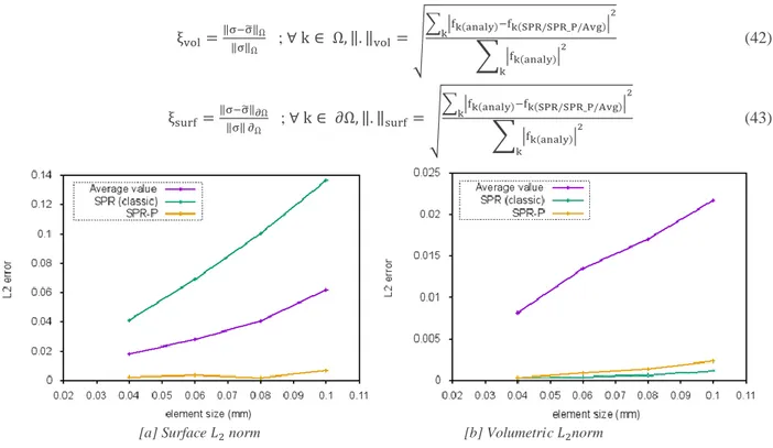
ξvol=‖σ−σ̃‖Ω ‖σ‖Ω ; ∀ k ∈ Ω, ‖. ‖vol= √ ∑ |fk(analy)−fk(SPR/SPR_P/Avg)| k 2 ∑ |fk(analy)|2 k (42) ξsurf=‖σ−σ̃‖∂Ω ‖σ‖ ∂Ω ; ∀ k ∈ ∂Ω, ‖. ‖surf= √ ∑ |fk(analy)−fk(SPR/SPR_P/Avg)| k 2 ∑ |fk(analy)|2 k (43)[a] Surface 𝐿2 norm [b] Volumetric 𝐿2norm
Figure 8. Comparison between some indirect transfer operators for function 𝑓2(𝑥, 𝑦, 𝑧) = 𝑥 ∗ 𝑦 ∗ 𝑧
Fig. 8 presents the volume and surface error values for SPR, SPR-P and Average recovery operator obtained for the linear function 𝑓2(𝑥, 𝑦, 𝑧) for several meshes with uniformly decreasing element sizes.
Figure8-a and 8-b, shows how the SPR technique values represent an improvement with respect to the analytic values inside the domain, in comparison with the other techniques; but this improvement is not enough to ensure a good surface error prediction. This verdict is well known when the standard SPR technique is applied to boundary points, especially for coarse meshes. In order to reduce the surface error booth, SPR-P and Average recovery technique can be used. Also, we can note that the error estimation both on surface and inside the domain illustrates better results with SPR-P recovery compared to the Average recovery technique. Similar conclusions are drawn using others analytic functions, such as quadratic, trigonometric and exponential. The corresponding comparison can be seen in Table 1.
For this work and in order to combine the advantage of these methods the SPR technique will be used to transfer the variables inside the domain and the SPR-P technique will be used to transfer the surface ones.
Tab 1.The slope of SPR-P and Average recovery operators with linear, quadratic, trigonometric and exponential functions
5 ADAPTIVE REMESHING METHODOLOGY
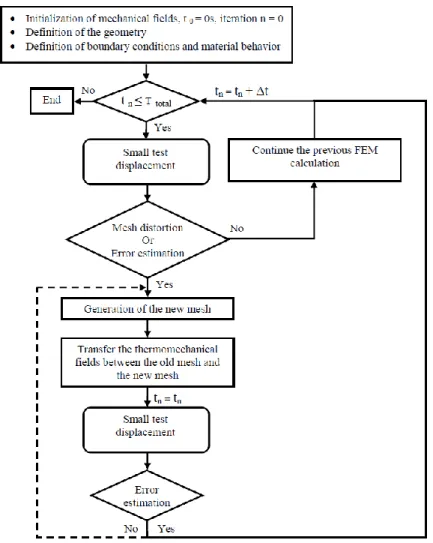
The proposed automatic adaptive remeshing strategy is presented in fig.9 and tested by solving two numerical examples under large inelastic deformations and high strain localization. The purpose of these examples is to illustrate the efficiency of the adaptive remeshing scheme adopted to optimize the mesh according to the aimed
12
prediction and to improve a good quality of elements in each step-time. In this work and similar to [Zeramdini 16], an element is classified as being distorted if one of his dihedral angles is larger than 160° or smaller than 10°, or if the ratio of element edges is smaller than 0.2.
Figure 9. Flow chart of the FE-simulation for 3D remeshing module
Only for the first step, the initial finite elements discretization using a tetrahedral element is provided. Then, for each time step an ABAQUS/Explicit FE calculation is performed with a small test displacement, and the resulting simulation is analyzed through a posteriori error estimators and element quality. If the estimated elementary error and / or the number of distorted elements does not exceed a given threshold, the previous FE simulation will be continued. Else, the mesh is then modified automatically (refined and / or coarsened) according to the constantly changing physical fields and geometrical shape and a new solution for this loading sequence is computed. For each time step, this process is repeated many times until the mesh no longer changes and/or the error level has been reached. Finally, all field variables are transferred from the old mesh to the new one and the simulation is restarted from the previous time step. It should also be noted that after each time step, the boundary and loading conditions are generated according to the old step modification.
6 NUMERICAL RESULTS
6.1 Shear test
First, a shear test is used in order to validate the proposed methodology and study some numerical aspects. Then, a metal forming process of a complex geometry will be tested. In each case, both the tool and the parts are discretized
13
with tetrahedral elements C3D4T with thermomechanical coupling taken from ABAQUS element library. The mesh of the tools is selected before the first step and remains unchanged. However, the initial mesh of the work piece is a regular coarse mesh and will be automatically adapted during the FE process. In the adaptive process the smallest hmin and largest hmax element sizes are respectively 0.1mm and 1mm. The contact interface between the tools and the
parts is modelled by the classical Coulomb model with a constant friction coefficient η=0.2. Finally, material subroutine Vumat is implemented to predict the Johnson-Cook model [Johnson 85] at each Gauss point for titanium alloy Ti17. The mechanical properties are similar to those reported in Reference [Ayed 16].
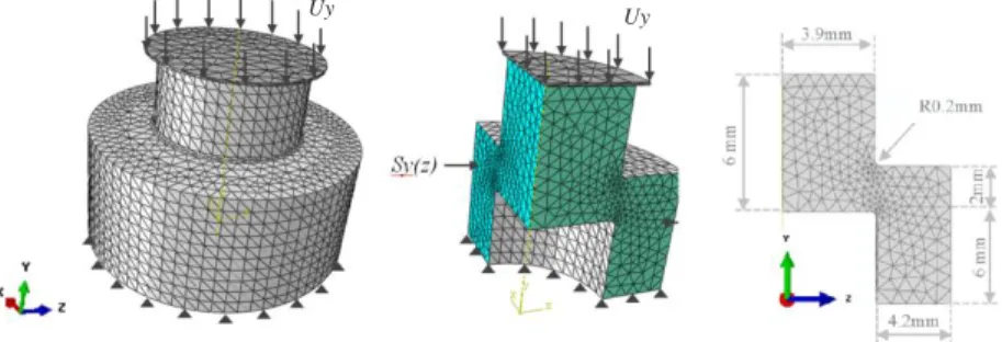
Figure 10. Geometry and boundary conditions of the specimens used in shear test
For the shear test, the geometry dimensions and boundary conditions are given in Fig.10. According to the symmetry conditions in a 3D configuration, only one quarter of the workpiece is modeled. To illustrate the efficiency of the adaptive strategy under large inelastic deformations and high strain localization, two uniform displacements of the rigid tool has been analyzed. All the adaptive procedure starts with 2493 uniformly distributed elements (Fig.11-a). Also, in order to attend the convergence of the FE solution and to study the influence of the element size on the stability of load, three target errors of 1%, 0.1%, and 0.03% have been used in the adaptive process. In this adaptive process, the smallest hmin and largest hmax element sizes are 0.1mm and 1mm respectively.
[a] Initial coarse mesh; 2493 tetrahedral elements
[b] u=0 mm [c] u=0.06 mm [d] u=0.014 mm Figure 11. Meshes at different instants with different targets errors
Target Error 1% Target Error 0.03% Target Error 1% Target Error 0.03% Target Error 1% Target Error 0.03% 1 6 0 0 tetr a h ed ra l elem en ts 1 0 6 7 0 0 tetr a h ed ra l elem en ts 1 6 6 0 tetr a h ed ra l elem en ts 9 4 5 7 2 tetra h ed ra l elem en ts 842 tetra h ed ra l elem en ts 9 7 8 5 7 tetra h ed ra l ele me n ts Uy Uy
14
Fig.11-b shows the final mesh obtained after four adaptive remeshing loops that can be compared with the initial one Fig11-a. This adaptive remeshing loop is adopted at every time step taking the adaptive deformed mesh in the previous step as the initial mesh. It can be observed how the adapted mesh concentrates additional elements in the critical zones whereas the number of elements in the rest of the domain remains practically unaltered or decreased. We can note that the element size increases and the number of elements decreases with increasing the imposed target error.
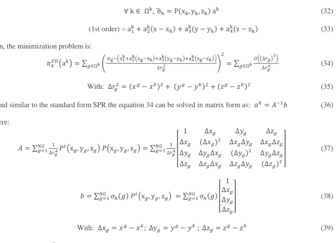
Figure 12. Comparison of load–displacement curves of mechanical tests using different deformation rate: 1mm/s and 100 mm/s
The comparison between the numerical load–displacement curves and published experimental data [Ayed 16] with different deformation rate 1 mm/s and 100 mm/s are shown in Fig12. At Fig.12-a, it can be shown that the smallest target error 0.03% is much more efficient in terms of convergence and accuracy of the FE solution in comparison with the large values 0.1% and 1%. However, even with this small target error 0.03% the system is not in mechanical equilibrium anymore. In fact, the numerical curves show a small fluctuation in the load-displacement response after each remeshing step which can be caused by a small degree of numerical diffusion during the transfer of variables between subsequent meshes. Also, we can note that the level of fluctuation decreases with the decease of the target error used in the adaptive process. This non-smooth pattern fluctuation is also observed using various others approaches such as average values, closest point technique [Zeramdini 16], Superconvergent Patch Recovery (SPR) [Khoei 07] or the unique element method (UEM) [Hu 98].
In Fig.12-b, we consider the same shear test as previously presented in Fig.12-a, but the shear test is performed under a high deformation rate of 100 mm/s. We can note that more critical results of mechanical instability load– displacement curves results are given under high deformation rate in comparison to the low one.
6.2 Equilibrium process
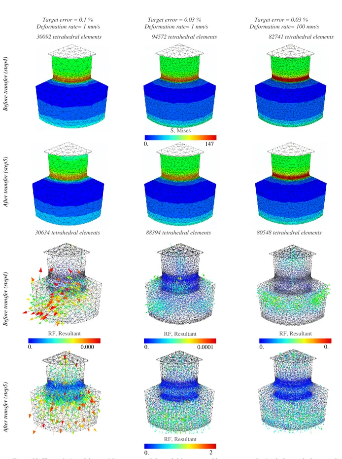
In order to solve the problem of this numerical instability, the results obtained before and after data transfer process between two successive meshes are compared. In Fig.13, the first row and the second one show the distribution of the von Mises stress components at integration points in each element; the third row and the fourth one show the value of internal forces at tetrahedral element nodes (equation 44).
𝑓𝑖𝑛𝑡= [ 𝑓𝑥𝑖𝑛𝑡1 𝑓𝑦𝑖𝑛𝑡1 𝑓𝑧𝑖𝑛𝑡1 ⋮ 𝑓𝑥𝑖𝑛𝑡𝑛𝑛𝑡 𝑓𝑦𝑖𝑛𝑡𝑛𝑛𝑡 𝑓𝑧𝑖𝑛𝑡𝑛𝑛𝑡] = ∫ 𝐵𝑇 𝜎̃ 𝑑𝑉 𝑉 = 1 6∫ ∫ ∫ 𝐵 𝑇 𝜎̃ 1 −1 𝑑𝑒𝑡[𝐽] 𝑑𝜉 𝑑𝜂 𝑑𝛿 = 1 −1 1 −1 1 6𝐵 𝑇 𝜎̃ det[J] ∫ ∫ ∫ dξ dη dδ1 −1 1 −1 1 −1 (44)
Where B and J are the spatial derivatives and the Jacobian matrix of the FE shape function, respectively.
15
Target error = 0.1 % Target error = 0.03 % Target error = 0.03 % Deformation rate= 1 mm/s Deformation rate= 1 mm/s Deformation rate= 100 mm/s 30092 tetrahedral elements 94572 tetrahedral elements 82741 tetrahedral elements
30634 tetrahedral elements 88394 tetrahedral elements 80548 tetrahedral elements
Figure 13. The evolution of the von Mises stress and the nodal force caused by stress smoothening before and after transfer at the same displacement u= 0.08 mm
0.000 5 0. 0 RF, Resultant 0.0001 4 0. 0 RF, Resultant 0. 5 0. 0 RF, Resultant Af te r t ra n sf er (s te p 5 ) Be fo re tra n sf er (s te p 4 ) Af te r tr a n sf er (s te p 5 ) Be fo re t ra n sf er ( st ep 4 ) 2 0 0. 0 RF, Resultant 147 3 0. 0 S, Mises
16
The second row in Fig.13 show a good continuous evolution of the von Mises stress after the transfer, due to the stress smoothening. However, only with small target error test, very small smooth diffusion can be seen. Before meshing, the nodal forces in the old mesh are very small since the explicit solver is used as shown in the third row and equation 45. However, it is not the case after remeshing specially in highly stain regions as shown in the fourth row. At this stage the main cause of the unbalanced system is due to the non-equilibrated forces at element nodes caused by stress smoothening in element. These nodal forces were self-equilibrated before transfer of state variables because the previous converged state was valid only for the old mesh (equation 45), but became external forces after transfer and are no longer in self-equilibrium with the new equilibrium equations (equation 46).
div (σoldel ) − moldn . γoldn = 0 (45) div (σnewel ) − mnewn . γnewn ≠ 0 (46) From fig.12 and fig.13, it can be construed that if the rate deformation or the elements size used during the numeric simulation is sufficiently small, mechanical equilibrium can be established again at small time increment, because the transfer error is too small. However, in these two cases, the CPU cost will increase. In the case of high rate deformation, the remeshing process must not be used because the numerical instability will be amplified (fig.14) even if the transfer error is too small. That is, the non-equilibrated forces at element nodes caused by stress smoothening are too small (third row in fig.13).
So, to restore equilibrium with the new boundary conditions the unbalanced internal forces must be removed. However, if they are eliminated at once, often the following iterations are found in mechanical imbalance,especially for coarse meshes. Analogy example of Spring-mass system can be helpful to solve the equilibrium problem. In fact, when a spring is stretched or compressed by a mass, the spring develops a restoring force. Only if this restoring force is small or relaxed the Spring-mass system can easily reach back to equilibrium. From this idea, a relaxation procedure has been implemented during the next step where these unbalanced nodal forces are removed successively by series of analytic function with decreasing coefficients. Note that only the values of dynamic nodal force mnewn . γnewn are kept. Where mnewn is the nodal mass of the new mesh discretization and the new acceleration values at the nodal points γnewn are computed by an interpolation of the old nodal acceleration via the FE shape function. The obtained results are presented in fig.14.
It is obvious in fig.14 that the equilibrium recovery proposed in this work allows to restore equilibrium after each meshing step. In terms of convergence under high and low rate deformation, the computed load/displacement responses obtained with equilibrium process give a good approximation of the experimental solution compared to the one obtained by only direct transfer.
17
Figure 14. Comparison of load–displacement curves of mechanical tests before and after equilibrium
From these results, it can be concluded that the use of adaptive mesh process coupled with the proposed equilibrium recovery has the better results compared to the use of standard one, for which the equilibrium recovery process is not imposed.
6.3 Metal Forming Processes
The metal forging is simulated with Abaqus 6.13 software. The half of geometry and boundary conditions are shown in fig. 15.According to the symmetry conditions, only an eighth workpiece is modeled.
Figure 15. Geometry, boundary conditions, and initial finite elements discretization.
In order to demonstrate the interest and efficiency of adaptive remeshing at a more complex geometries level, the same metal forging simulation is carried out with the presented mesh adaptation strategy (adaptive case) and without mesh adaptation (standard case). One of the critical ingredients in any FEM process is the mesh discretization. In fact, a severe mesh distortion can occur during the standard simulation especially with constant coarse mesh. However, it is not the case with the adaptive test because the mesh is automatically adapted according to the constant change (physical fields and geometrical shapes). That’s why the initial mesh of the standard test must be optimized in some critical zones as shown in fig. 16. This comparison can improve a first advantage of using the adaptive process to avoid excessive mesh refinement, and present a good filling of the die matrices.
The numerical results presented in fig. 16 show the efficiency of the adaptive remeshing process. In fact, from the beginning of the simulation to the end, a good quality of elements is proved with the adaptive strategy. However, a severe mesh distortion is observed without mesh adaptation. With the adaptive process, the simulation ends with zero element distortion compared to 6325 distorted elements without remeshing.
18
With mesh adaptation Local element quality without mesh adaptation
85178 tetrahedral elements; u= 0 mm 85178 tetrahedral elements; u= 0 mm
105799 tetrahedral elements; u= 0.75 mm 85178 tetrahedral elements; u= 0.75 mm
142783 tetrahedral elements; u= 1.6 mm 85178 tetrahedral elements; u= 1.6 mm
90515 tetrahedral elements; u= 1.85 mm 85178 tetrahedral elements; u= 1.85 mm
Figure 16. Meshes at different tool displacement in the left with mesh adaptation and in the right without mesh adaptation
215 0 0. 0 S, Mises 1 2 1 2 1 2 2 1
19
As it was noted above, each element size can be considered as optimal only if the procedures of successive mesh adaptation give modification coefficient are close to 1. So, the remeshing iteration is repeated many times until the total number of optimal elements does not exceed a given threshold. For this metal forging simulation, the target threshold of optimal elements number is selected as 75% and more strict area of modification coefficient is chosen
3
4≤ R
e≤5
4 compared to the reference coefficient proposed by Ladevèze [Ladevèze 01] which is 2
3≤ R
e≤3 2 .
Figure 17 shows that the both simulations start with the same number of optimal elements. With the standard process, the percentage of optimal element decrease after each load displacement step until the end of simulation. In this stage, only 23% of elements are conformed to the target error. However, with the adaptive process if the percentage of optimal element is above the given threshold 75%, the previous FE simulation will be continued. Else, the mesh is then modified automatically according to the constant change of physical fields and geometrical shape. Another strong point of the presented process is that for each time step, the number of remeshing-iterations is not fixed, but it is automatically adapted, as shown in fig. 17. This characteristic can avoid the useless iteration and reduce time cost. For example for the first meshing step four iterations are performed; for the second and third meshing step two iterations; for the fourth meshing step only one iteration is used.
Figure 17. The evolution of the percentage of optimal Figure 18. Comparison of load–displacement curves of element with and without mesh adaptation forming tests with and without mesh adaptation
The evolution of numerical load–displacement curves with and without adaptive remeshing is compared in fig. 18. At the beginning of simulation both EF simulations give similar results. However, it is not the case at the end of test. This difference may be caused by the presence of excessive mesh distortion in the standard test (without adaptive remeshing). As can be seen in figs 16 and 19, these mesh distortions favors the displacement of elements in the second direction compared to the first one. In other words, the contact area between the rigid tool and the workpiece will not be the same especially in the second zone (II), which have a strongly effect on the normal load.
With mesh adaptation u= 1.6 mm without mesh adaptation u= 1.6 mm
Figure 19. The effect of mesh-distortion onthe geometry of the workpiece
(1) (2) Zone (I) Zone (II) Zone (I) Zone (II)
20
7 CONCLUSION
In this paper, an automatic adaptive remeshing method based on local mesh modification has been presented to simulate various 3D metal forming processes in large elastoplastic deformations. This process has been implemented with a small test displacement step by step in order to adapt automatically to the constantly changing physical fields and geometrical shapes. At each time-step, the remeshing iteration is repeated many times until the total number of optimal elements does not exceed a given threshold. This characteristic can avoid the useless iteration and reduce time cost. To avoid numerical diffusion during the mapping of variables, data transfer error is examined using analytical functions such as linear, quadratic, trigonometric and exponential with volumetric L2 error norms and surface one. The results show that these techniques illustrate different efficiency. So, in order to combine the advantage of these methods the SPR technique will be used to transfer the variables inside the domain and the SPR-P technique will be used to transfer the surface ones. Without equilibrate process, the numerical load-displacement curves under large displacement and/or high deformation rate show that after each remeshing step the system is not in mechanical equilibrium anymore. In fact, the numerical curves show a small fluctuation in the load-displacement response after each remeshing step. But with the proposed equilibrated process a good agreement with experimental data has been observed and the imbalance fluctuations are reduced significantly. Also, a good quality of elements is proven with the adaptive strategy, but a severe mesh distortion is observed without mesh adaptation which can significantly reduce the efficiency of numerical result. Finally, the overall results are very encouraging and show the efficiency and robustness of the proposed strategy to avoid mesh distortion and to simulate more complex geometry levels with a better filling of the die matrices compared to the standard approach. However, several points can be improved such as damage evolution. Moreover, it’s important to taking into account the contacts management between the piece and rigid tool to avoid any interpenetration.
REFERENCES
1. [Ainsworth 97] M. Ainsworth and J. T Oden, « A posteriori error estimation in finite element analysis ». Computer Methods in Applied Mechanics and Engineering, Vol. 142, pp.1-88, 1997.
2. [Ayed 16] Y. Ayed, G. Germain, A. Ammar and B. Furet, « Thermo-mechanical characterization of the Ti17 titanium alloy under extreme loading conditions ». The International Journal of Advanced Manufacturing Technology, Springer-Verlag London 2016.
3. [Babuška 78] I. Babuška and W. C. Rheinbildt, « A posteriori error estimates for the finite element method ». International Journal For Numerical Methods In Engineering, Vol. 12, pp. 1597-1615, 1978.
4. [Babuška 94] I. Babuška, T. Strouboulis, C. S. Upadhyay, S. K. Gangaraj and K. Copps, « Validation of a posteriori error estimators by numerical approach ». International Journal For Numerical Methods In Engineering, Vol. 37, pp. 1073-1123, 1994.
5. [Boussetta 04] R.Boussetta and L.Fourment, « A Posteriori Error Estimation And Three‐dimensional Adaptive Remeshing: Application To Error Control Of Non‐Steady Metal Forming Simulations ». AIP Conference Proceedings, pp.712-2246, 2004.
6. [Boussetta 06] R.Boussetta, T.Coupez and L.Fourment, « Adaptive remeshing based on a posteriori error estimation for forging simulation ». Computer Methods in Applied Mechanics and Engineering, Vol. 195, pp 6626–6645, 2006. 7. [Ciarlet 78] P.G. Ciarlet, « The Finite Element Method for Elliptic Problems». North-Holland Publishing Company,
Amsterdam, New York, pp, 534, 1978.
8. [Diez 07] P. Diez a, G.Calderon, « Remeshing criteria and proper error representations for goal oriented h-adaptivity ». Computer Methods in Applied Mechanics and Engineering, Vol. 196, pp. 719–733, 2007.
9. [Dureisseix 06] D. Dureisseix and H. Bavestrello, « Information transfer between incompatible finite element meshes: Application to coupled thermo-viscoelasticity». Computer Methods in Applied Mechanics and Engineering, Vol. 85, pp. 6523-6541, 2006.
10. [Hochard 95]Ch. Hochard, D. Peric, M. Dutko and D.R.J. Owen, « Transfer operators for evolving meshes in elasto-plasticity ». Proceeding of Computational Plasticity Fundamentals and Applications, Barcelona, pp. 2331-2339, 1995. 11. [Hu 98] Y. Hu and M.F. Randolph, « H-adaptive FE analysis of elasto-plastic non-homogeneous soil with large
deformation ». Computers and Geotechnics. Vol. 23, pp. 61-83, 1998.
21
13. [Khoei 07] A.R. Khoei, S.A. Gharehbaghi, A.R. Tabarraie and A. Riahi, « Error estimation, adaptivity and data transfer in enriched plasticity continua to analysis of shear band localization ». Applied Mathematical Modelling. Vol. 31, pp. 983-1000, 2007.
14. [Kumar 15] S.Kumar, L.Fourment and S.Guerdoux, « Parallel, second-order and consistent remeshing transfer operators for evolving meshes with superconvergence property on surface and volume ». Finite Elements in Analysis and Design, Vol. 93, pp 70–84, 2015.
15. [Ladevèze 86] P. Ladevèze, G. Coffignal and J. P. Pelle, « Accuracy of elastoplastic and dynamic analysis ». In I. Babuška. O. C. Zienkiewicz, J. Gago and E. R. de A. Oliveira, « Accuracy Estimates and Adaptive Refinements in Finite Element Computations ». John Wiley & Sons Ltd (1986) Chap. 11, pp. 181-203.
16. [ladvèze 01] Pierre Ladevèze and Jean-Pierre Pelle, « Mastering Calculation in Linear and Nonlinear Mechanics ». Publisher Springer 2004,
17. [Liszka 80] T. Liszka and J. Orkisz, « The finite differences method at arbitrary irregular grids and its application in applied machanics ». Computer & Structure, Vol. 11, pp. 83-95, 1980.
18. [Liszka 84] T. Liszka, « An interpolation method for an irregular net of nodes ». International Journal for Numerical Methods in Engineering, Vol. 20, pp. 1599-1612, 1984.
19. [Lo 91] S. H. Lo, « Volume discretization into tetrahedra-1. Verification and orientation of boundary surfaces ». Computers & Structures, Vol. 39, pp. 493-500, 1991.
20. [Lo 91a] S. H. Lo, « Volume discretization into tetrahedra-II. 3D triangulation by advancing front approach ». Computers & Structures, Vol. 39, pp. 501-511, 1991.
21. [Peric 96] D. Peric, Ch. Hochard I, M. Dutko and D.R.J. Owen, « Transfer operators for evolving meshes in small strain elasto-placticity ». Computer Methods in Applied Mechanics and Engineering, Vol. 137, pp. 331–344, 1996.
22. [Verfurth 99] R. Verfurth, « A Review of A Posteriori Error Estimation Techniques for Elasticity Problems ». Computer Methods in Applied Mechanics and Engineering, Vol. 176, pp. 419–440, 1999.
23. [Wiberg 94] N-E. Wiberg, F. Abdulwahab and S. Ziukas, « Enhanced Superconvergent Patch recovery incorporating equilibrium and boundary conditions ». International Journal for Numerical Methods in Engineering, Vol. 37, pp. 3417-3440, 1994.
24. [zeramdini 16] B. Zeramdini, C. Robert, G. Germain, and T. Pottier, « Simulation of metal forming processes with a 3D adaptive remeshing procedure ». AIP Conference Proceedings 1769, 200018, 2016.
25. [Zienkiewicz 87] O. C. Zienkiewicz and J. Z. Zhu, « A simple error estimator and adaptive procedure for practical engineering analysis ». International Journal For Numerical Methods In Engineering, Vol. 24, pp. 337-357, 1987. 26. [Zienkiewicz 92] O. C. Zienkiewicz and J. Z. Zhu, « The Superconvergent Patch Recovery (SPR) and adaptive finite
element ». Computer Methods in Applied Mechanics and Engineering, Vol. 101, pp.207-224, 1992.
27. [Zienkiewicz 92a] O. C. Zienkiewicz and J. Z. Zhu, « The Superconvergent Patch Recovery and a posteriori error estimates. Part 1: The recovery technique ». International Journal For Numerical Methods In Engineering, Vol. 33, pp. 1331-1364, 1992.
28. [Zienkiewicz 92b] O. C. Zienkiewicz and J. Z. Zhu, « The Superconvergent Patch Recovery and a posteriori error estimates. Part 2: Error estimates and adaptivity ». International Journal For Numerical Methods In Engineering, Vol. 33, pp. 1331-1364, 1992.
![Figure 12. Comparison of load–displacement curves of mechanical tests using different deformation rate: 1mm/s and 100 mm/s The comparison between the numerical load–displacement curves and published experimental data [Ayed 16] with differen](https://thumb-eu.123doks.com/thumbv2/123doknet/7427117.219501/15.918.111.792.232.476/comparison-displacement-mechanical-different-deformation-comparison-displacement-experimental.webp)