is an open access repository that collects the work of Arts et Métiers Institute of Technology researchers and makes it freely available over the web where possible.
This is an author-deposited version published in: https://sam.ensam.eu Handle ID: .http://hdl.handle.net/10985/10197
To cite this version :
Ion LEAHU-ALUAS, Farid ABED-MERAIM - A proposed set of popular limit-point buckling benchmark problems - Structural Engineering and Mechanics - Vol. 38, n°6, p.767-802 - 2011
Any correspondence concerning this service should be sent to the repository Administrator : [email protected]
A proposed set of popular limit-point buckling
benchmark problems
Ion Leahu-Aluas1,2 and Farid Abed-Meraim*1
1LEM3, UMR CNRS 7239, Arts et Métiers ParisTech, 4 rue A. Fresnel, 57078 Metz Cedex 03, France 2Georgia Tech Lorraine, Georgia Institute of Technology, 2-3 rue Marconi, 57070 Metz, France
Abstract. Developers of new finite elements or nonlinear solution techniques rely on discriminative benchmark tests drawn from the literature to assess the advantages and drawbacks of new formulations. Buckling benchmark tests provide a rigorous evaluation of finite elements applied to thin structures, and a complete and detailed set of reference results would therefore prove very useful in carrying out such evaluations. Results are usually presented in the form of load-deflection curves that developers must reconstruct by extracting the points, a procedure which is often tedious and inaccurate. Moreover the curves are usually given without accompanying information such as the calculation time or number of iterations it took for the model to converge, even though this type of data is equally important in practice. This paper presents ten different limit-point buckling benchmark tests, and provides for each one the reference load-deflection curve, all the points necessary to recreate the curve in tabulated form, analysis data such as calculation time, number of iterations and increments, and all of the inputs used to obtain these results.
Keywords: finite element; nonlinear analysis; limit-point buckling benchmarks; post-buckling; path-following strategy; large rotations.
1. Introduction
For the past two decades, many finite element programs have been developed with the aim of simulating, as efficiently and as accurately as possible, various kinds of mechanical and coupled problems. These in-house or commercial software packages usually incorporate different libraries of finite elements and make use of diverse nonlinear solution techniques. There is a widely recognized need for testing and comparing the above-mentioned formulations and strategies. The performance of newly developed finite elements is commonly assessed based on a variety of test problems, ranging from linear analyses to geometric as well as material nonlinear benchmarks. A carefully designed set of standard linear test problems was proposed for such evaluations by MacNeal and Harder (1985). These benchmarks have proven to be very useful and have been used extensively to decide whether a proposed formulation is free from the most important weaknesses that affect accuracy and efficiency; namely spurious mechanisms (also known as rank deficiencies) and locking phenomena. Subsequent publications (Hitchings et al. 1987, Prinja and Clegg 1993) by the *Corresponding author, Professor, E-mail: [email protected]
UK’s National Agency for Finite Element Methods and Standards (NAFEMS) confirmed that finite element validation has become a matter of primary concern. More recently, Sze et al. (2004) proposed a detailed set of popular benchmark problems, for the specific case of geometric nonlinear analysis of thin structures.
The purpose of the current work is to provide developers of new finite element models or new nonlinear solution methods the numerical reference solutions for the most commonly used limit-point buckling benchmark tests. The plots and tables provided in this article are the converged mesh solutions, obtained by the careful analysis of several accurate and reliable shell elements. This information may therefore be used with confidence as a reference for the aforementioned benchmark tests. This implies that the given curves are the ABAQUS state of the art in terms of limit-point buckling simulations. No experimental results are presented in this article. Finally, for each test, two curves are given; the converged mesh and the mesh refined by a factor of two in the relevant directions when compared to the converged mesh. This is done in order to show that the converged mesh density is sufficient. Eight out of the ten benchmark tests have already been studied in the literature, and two of them are new. These new proposed benchmark tests deal with elastic-plastic limit-point buckling.
Since most authors provide results in terms of load-displacement curves, the interested developers and researchers have to extract the data points from these curves and then recreate them in order to be able to test their new finite element models or nonlinear solution methods. This is not only a tedious task, but more importantly, it is often an inaccurate one. Therefore, one of the goals of this article will be to eliminate this intermediate step by providing the results in tabulated form, together with the load-deflection curves. The points provided in the tables are all of the points needed to recreate the original curve.
The load-displacement results by themselves do not suffice when comparing new finite element models or nonlinear solution methods. The computing time, number of iterations, number of increments, and number of cutbacks are also needed in order to compare the speed and relative ease of convergence of the new versus the old techniques. Therefore this type of analysis data is provided in the article as well, which corresponds to the convergence criterion taken equal to its default value (see the detailed documentation in ABAQUS (2007) and the discussion in Section 4.3). To put the calculation times into perspective, all the tests were run on a Dell Precision 380 personal computer with a 2.4 GHz Intel Xeon CPU and 2 GB of RAM. The nonlinear solution method used was a modified path-following Riks method, implemented in ABAQUS. The inputs for the modified Riks method are also reported so that the reader has all the information necessary to recreate the benchmark tests.
2. General comments on limit-point buckling
Typical thin structures are prone to instability phenomena that may occur prior to their conventional strength limit. Such structural instabilities are known as buckling, which in theory is characterized by a sudden deflection of a structure (usually thin) when subjected to compressive loads. Such failure modes occur when the compressive load reaches a critical value. In practice, this phenomenon involves significant changes in the shape of the structure with geometric nonlinear effects. Besides the well-known sensitivity of buckling to geometric imperfections, it is also known to be very sensitive to boundary conditions. It is also well-known that critical points are classified
into limit points and bifurcation points. Over the last three decades, considerable effort has been devoted to the detection of such singular points and the associated post-buckling behavior. Various criteria and efficient algorithms have been developed to deal with this issue as demonstrated by the comprehensive literature in this field (see, for example, Koiter 1945, Timoshenko and Gere 1961, Hutchinson and Koiter 1970, Thompson and Hunt 1973, Budiansky 1974, Abed-Meraim 1999, Abed-Meraim and Nguyen 2007).
Limit-point buckling, also called snap-through buckling, is the type of buckling whereby there is a sudden large movement (jumping) in the direction of the loading, as opposed to bifurcation buckling, where the bifurcated branch intersects the fundamental path (branching), inducing significant changes in the shape of the structure (see Fig. 1). In this work, our attention is focused on limit-point buckling. As stated earlier, the modified path-following Riks method, which is the algorithm implemented in ABAQUS for solving this type of problem, is the method used to obtain the load-deflection curves. Before the benchmark tests are presented, it is important to understand how this algorithm works and how the different inputs affect the way the simulation is carried out. The discussion below is a brief, simplified introduction to the parameters important for the modified Riks algorithm, as implemented in ABAQUS (2007). For further information, the reader is invited
Fig. 1 Schematic representation of bifurcation-type buckling versus limit-point buckling
Fig. 2 (a) Typical load-displacement curve for through, (b) typical load-displacement curve for snap-back
to consult the ABAQUS documentation and articles by Riks (1979), Crisfield (1981) and Ramm (1981).
In order to capture the complex load-displacement response, which can exhibit a decrease in load and/or displacement as the solution evolves (see Fig. 2), the equilibrium path is computed by including the load magnitude as an additional unknown in the formulation of the problem. The result of this is proportional loading, as all load magnitudes then vary with a single scalar parameter, called the load proportionality factor. For some of the benchmark cases, the results are given in terms of this load proportionality factor, which is given by ABAQUS as a history output. The method described here is also called an arc-length method because the equilibrium path in the new space, defined by the nodal variables and the loading parameter, is determined by using this so-called arc-length. The arc-length itself multiplies the load by a load factor, allowing both the load and the displacement to vary throughout the time step.
Due to the nature of this technique, the loading applied to the structure is only used as an indication of the direction of loading. The actual load applied in the first increment is the product of this load and the initial arc-length, which is one of the inputs of this procedure. If an increment converges easily, the arc-length in the subsequent increment will be increased by a factor of 1.5. In cases of snap-back, it is possible that by the time the snap-back region is reached, the arc-length is so large that the next point found is further along on the equilibrium path than this snap-back region. In this case, the algorithm will respond by erroneously skipping over this region. This hazard is avoided by limiting the maximum arc-length (whose default value is 1036). It is often necessary to first run a model with the default value and then reduce it gradually to see how the resulting curve is affected. If a small maximum arc-length value is used from the beginning, it is possible that more points will be calculated on the equilibrium path than necessary to trace the curve, which could significantly increase the calculation time.
The number of increments, the number of iterations and the number of cutbacks are all indicators of the relative ease of convergence of a problem. The number of cutbacks is especially useful, as it shows how many times the size of the increment had to be reduced due to the inability of the solver to find a solution for the given increment size. This analysis data depends obviously on the tightness of the convergence criterion, the latter is left to its default value, specified in the ABAQUS documentation (2007), throughout the paper, unless explicitly specified otherwise (see Section 4.3 for more details).
The stopping criterion used is also different from other solution techniques. There are in fact three different ways for a simulation to come to completion. The analysis is terminated when it reaches either an imposed node displacement, an imposed load proportionality factor, or when the (predefined) maximum number of increments is reached. In certain cases, the end point of the load-displacement curve will surpass the imposed stopping criterion. This is because the arc-length for the last segment may be very large. ABAQUS will continue the analysis until the last point is equal to or greater than the stopping criterion, which is to say that ABAQUS will not adjust the final arc-length in order to exactly meet the stopping criterion. The final important point is that the ABAQUS keyword ‘NLGEOM’, which stands for “nonlinear geometry,” must be used for all these analyses in order to take second order effects into account.
All of the previously discussed parameters were considered and optimized for these benchmark tests, in order to guarantee that the solutions obtained are the best ones possible and that the reader can use them with confidence.
3. Benchmark tests
Ten limit-point buckling benchmark tests, which cover a wide range of structures, boundary conditions, and loadings, are presented in this section. These include deep and shallow arches of various cross-sections, thin and thick cylindrical sections, beams, and frames. Hinged and clamped boundary conditions, as well as concentrated, pressure, and inclined loadings are investigated. Elastic-plastic behavior is also treated in the two new benchmark tests proposed at the end of this section. All of these benchmark problems exhibit some common features such as nonlinear pre-buckling and unstable pre-buckling behavior.
As expected, shell elements were found to be the best suited for this type of application and, in most cases, the converged meshes for the three shell elements tested gave the same load-deflection curve. The results stated for each benchmark test are therefore those corresponding to the most efficient element, i.e., the fastest one. Evidently, the accuracy of the solution always prevails over the speed of the calculation. The obtained results were always compared with other literature results in order to understand which element performed the best. Whenever the final result was found different from the one given in the literature, careful investigations of accuracy and convergence were performed with more expensive high-order elements. An analytical solution is available for several cases, however, the reader must keep in mind that all analytical solutions make use of one or more simplifying assumptions. Since much care was taken to arrive at the best numerical solution, a mismatch with a given analytical solution is probably due to one of the assumptions used to derive the latter solution over-simplifying the problem. Another important point regarding numerical solutions drawn from the literature is the fact that the results might be an average of results computed by several different pieces of software, which could introduce deviations to the load-displacement curve.
The nomenclature given below is employed throughout this article. Furthermore, the important features of all the ABAQUS elements tested are given in Table 1.
3.1 Clamped shallow circular arch subjected to pressure loading
The geometry of this test is shown in Fig. 3. Since the arch, the loading, and the boundary conditions are symmetric, only half of the geometry is modeled. An analytical solution for this problem is given by Schreyer and Masur (1966), and numerical solutions were also developed, notably by Sharifi and Popov (1971). The ABAQUS manual (2007) gives the numerical solution
Nomenclature and naming conventions
u Displacement length (l) Longest side of the structure
R Radius width (w) Side perpendicular to the loading direction P Applied load thickness (t) Side parallel to the loading direction E Elasticity modulus
ν Poisson’s ratio The mesh naming convention is length×width(×thickness) I Area moment of inertia
Table 1 Important features of the S4R, S4 and S4R5 shell elements, of the C3D8, C3D8I and C3D8R continuum elements, and the SC8R continuum-shell element
S4R S4 S4R5
Number of nodes 4 4 4
Integration points 1×n* 4×n* 1×n*
Degrees of freedom 6 (3 displacements, 3 rotations)
6 (3 displacements, 3 rotations)
5 (3 displacements, 2 rotations) Hourglass treatment Default stabilization Not applicable Not applicable
Applicable strain Finite Finite Small
Intended thickness Thin/thick Thin/thick Thin only
C3D8 C3D8I C3D8R SC8R
Number of nodes 8 8 8 8
Integration points 8 8 1 1×n*
Degrees of freedom 3 (displacements) 3 (displacements) 3 (displacements) 3 (displacements) Hourglass treatment Not applicable Not applicable Default stabilization Default stabilization
Applicable strain Finite Finite Finite Finite
Intended thickness Thin/thick Thin/thick Thin/thick Thin/thick *an arbitrary number (n) of integration points can be used through the thickness (the default value is five).
Fig. 3 Clamped shallow circular arch subjected to pressure loading, (a) geometric, material, and loading data, (b) initial and deformed configuration under maximum load, (c) solutions drawn from the literature and from the ABAQUS manual
obtained with beam elements. These solutions, given in terms of pressure versus normalized displacement (u/R), are shown in Fig. 3(c). This figure shows that the literature does not provide a complete picture of the post-buckling behavior. The results obtained with the ABAQUS linear beam element (B21) are very close to those given by Schreyer and Masur (1966), with the only slight differences occurring before buckling. Since this benchmark test deals with a 3D structure, one cannot assume that the correct results can be calculated using beam elements. Shell, continuum, and
Table 2 Riks analysis inputs for the clamped shallow circular arch subjected to pressure loading
Stopping criterion Initial arc-length Minimum arc-length Maximum arc-length Maximum load proportionality
factor of 0.4 0.05 10-5 0.1
Fig. 4 Load-displacement curves for the clamped shallow circular arch subjected to a pressure load. The plotted displacement is the vertical displacement of the pole of the arch
Table 3 (a) Results for the clamped shallow circular arch subjected to pressure loading, (b) analysis data (a)
−uy/R P [MPa] −uy/R P [MPa] −uy/R P [MPa] −uy/R P [MPa]
0.0000 0 0.0199 996 0.0449 717 0.0664 1418 0.0019 231 0.0243 958 0.0487 732 0.0697 1714 0.0039 431 0.0286 895 0.0525 781 0.0729 2075 0.0070 671 0.0329 828 0.0561 869 0.0112 883 0.0370 771 0.0596 1001 0.0155 982 0.0410 731 0.0630 1182 (b)
Element Mesh CPU time [sec] Number of increments Number of iterations
S4R 14×1 1.24 20 53
continuum-shell ABAQUS elements were therefore tested to obtain the reference solution. The Riks analysis inputs used to set up the ABAQUS simulation are summarized in Table 2.
The results obtained using shell elements are very close to the analytical solution. Fig. 4 shows the plot of pressure versus normalized displacement of the arch apex. Table 3 shows tabulated results as well as analysis data such as calculation time for the S4R element, which was the fastest out of the three ABAQUS linear shell elements tested.
3.2 Clamped-hinged deep circular arch subjected to a concentrated load
The characteristics of this test are presented in Fig. 5. One end of the arch is hinged, and the other one is clamped. DaDeppo and Schmidt (1975) provide the analytical solution for this problem, and it is also considered in the ABAQUS manual (2007). The solution is given in terms of normalized force (PR2/EI) versus normalized displacement (u/R), where (I = wt3/12). The displacement is given
Fig. 5 (a) Geometric, material, and loading data for the clamped-hinged deep circular arch subjected to a concentrated load, (b) evolution of the structure shape and of the load location, (c) DaDeppo and Schmidt (1975) analytical solution
for both the x and the y directions. Due to the asymmetry of the boundary conditions, the buckling will be asymmetric as well. Table 4 summarizes the Riks analysis inputs used for this test.
The results obtained with shell elements came closest to the analytical solution. Fig. 6 shows the plot of normalized load versus normalized displacement. Table 5 provides results in tabular form as Table 4 Riks analysis inputs for the clamped-hinged deep circular arch subjected to a concentrated load
Stopping criterion Initial arc-length Minimum arc-length Maximum arc-length Maximum central point displacement of
120 mm in the negative y direction 0.5 10-5 default value
Fig. 6 Load-displacement curves for the clamped-hinged deep circular arch subjected to a concentrated load Table 5 (a) Tabulated displacement and load results for the clamped-hinged deep circular arch subjected to a
concentrated load, (b) analysis data (a)
-ux/R -uy/R PR2/EI -ux/R -uy/R PR2/EI -ux/R -uy/R PR2/EI
0.000 0.000 0.000 0.513 0.774 7.042 0.612 1.140 9.024 0.023 0.031 0.869 0.543 0.869 7.581 0.619 1.158 8.972 0.065 0.083 1.956 0.569 0.967 8.171 0.626 1.172 8.818 0.132 0.159 3.060 0.590 1.057 8.705 0.633 1.184 8.542 0.216 0.257 4.016 0.594 1.075 8.809 0.639 1.192 8.120 0.336 0.417 5.101 0.599 1.093 8.897 0.644 1.198 7.557 0.436 0.590 6.054 0.605 1.118 8.993 0.646 1.200 7.237 (b)
Element Mesh CPU time [sec] Number of
increments Number of iterations Number of cutbacks S4R 48×1 3.99 33 168 3 S4R 96×1 6.56 36 195 7
well as analysis data such as calculation time.
3.3 Hinged thin cylindrical section subjected to a central concentrated load
This is a very popular benchmark test that has been considered by multiple authors (Crisfield 1981, Ramm 1981, Cho et al. 1998, Eriksson et al. 1999, Kim and Kim 2001, 2002, Sze and Zheng 2002, Areias et al. 2003, Boutyour et al. 2004, Sze et al. 2004, Kim et al. 2005, Alves de Sousa et al. 2006, Wardle 2006, 2008). The geometry of this test is presented in Fig. 7, while Table 6 gives the basic simulation inputs for the path-following algorithm. The lateral, straight sides are hinged, while the two other curved sides are free. Only numerical results are available for this particular test, given in terms of load versus displacement at the middle point of the structure, where the load is applied. Fig. 7 also provides a plot of the results obtained by several authors. Notice that Eriksson et al. (1999) and Alves de Sousa et al. (2006) obtained slightly different solutions than the other authors. Despite the symmetry of the problem, the geometry was modeled in its entirety because some authors (Wardle 2006, 2008) noticed that this particular test could also exhibit a bifurcation
Fig. 7 Hinged thin cylindrical section subjected to a central concentrated load, (a) geometric and loading data, (b) deformed configuration under maximum load, (c) solutions drawn from the literature
solution. This aspect will be further discussed in Section 4.
The three shell elements used here gave the same results, which were very close to those drawn from the literature. The S4R5 element had the fastest computation time. Fig. 8 shows the plot of load versus displacement, and Table 7 gives tabular results as well as relevant analysis data.
Table 6 Riks analysis inputs for the hinged thin cylindrical section subjected to a central concentrated load Stopping criterion Initial arc-length Minimum arc-length Maximum arc-length Maximum central point displacement of
30 mm in the negative y direction 0.1 10-5 0.2
Fig. 8 Load-displacement curves for the hinged thin cylindrical section subjected to a central concentrated load
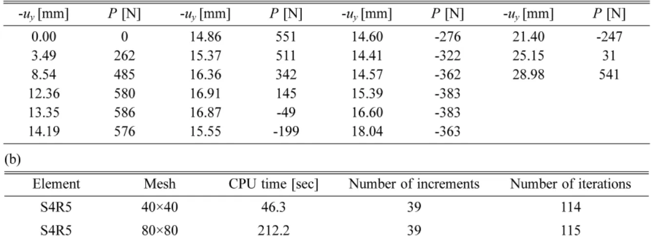
Table 7 (a) Displacement and load results for the hinged thin cylindrical section subjected to a central concentrated load, (b) analysis data
(a) -uy [mm] P [N] -uy [mm] P [N] -uy [mm] P [N] -uy [mm] P [N] 0.00 0 14.86 551 14.60 -276 21.40 -247 3.49 262 15.37 511 14.41 -322 25.15 31 8.54 485 16.36 342 14.57 -362 28.98 541 12.36 580 16.91 145 15.39 -383 13.35 586 16.87 -49 16.60 -383 14.19 576 15.55 -199 18.04 -363 (b)
Element Mesh CPU time [sec] Number of increments Number of iterations
S4R5 40×40 46.3 39 114
3.4 Hinged thick cylindrical section subjected to a central concentrated load
This test is the same as the previous one with the exception of the thickness, which is now twice as large (t = 12.7 mm). Several authors have examined this test (Klinkel and Wagner 1997, Sze and Zheng 2002, Legay and Combescure 2003, Sze et al. 2004, Kim et al. 2005). Only numerical results are available for this particular test, given in terms of load versus displacement at the middle point of the structure, where the load is applied. Fig. 9 and Table 8 give the important characteristics and input data used for this test.
Despite the symmetry of the problem, the entire geometry is again meshed according to the previous, similar-but-thin case. The results obtained with shell elements come closest to the
Fig. 9 Hinged thick cylindrical section subjected to a central concentrated load, (a) geometric and loading data, (b) deformed configuration under maximum load, (c) solutions drawn from the literature
Table 8 Riks analysis inputs for the hinged thick cylindrical section subjected to a central concentrated load Stopping criterion Initial arc-length Minimum arc-length Maximum arc-length Maximum central point displacement of
literature results. Fig. 10 shows the load versus displacement plot. Tabulated results as well as analysis data are provided in Table 9.
3.5 Lee’s frame
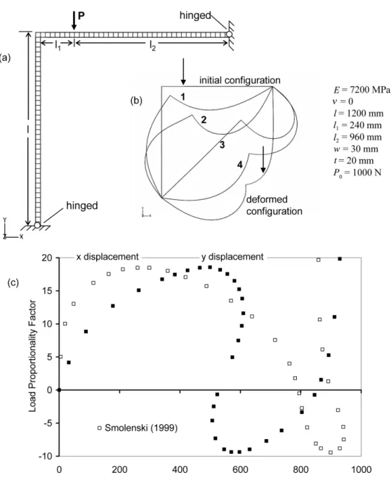
This benchmark test is named after S.L. Lee, who was the first to look at this problem (Lee et al. 1968). The problem has subsequently been examined by several authors (Smolenski 1999, Planinc and Saje 1999). The geometry and loading (concentrated load) are shown in Fig. 11. The input data for the Riks algorithm is given in Table 10. The results are given in terms of load proportionality factor (LPF) versus displacement in the x and the y directions at the point where the load is applied. Fig. 10 Load-displacement curves for the hinged thick cylindrical section subjected to a central concentrated
load
Table 9 (a) Tabulated displacement and load results for the hinged thick cylindrical section subjected to a central concentrated load, (b) analysis data
(a) -uy [mm] P [N] -uy [mm] P [N] -uy [mm] P [N] -uy [mm] P [N] 0.00 0 5.14 1562 15.07 1542 22.82 883 0.25 99 7.21 1939 15.80 1255 24.77 1378 0.50 194 9.07 2149 16.54 976 26.90 2134 0.88 332 10.70 2220 17.37 738 29.18 3192 1.43 528 12.10 2172 18.37 573 31.58 4594 2.25 796 13.27 2028 19.61 518 3.44 1145 14.25 1809 21.09 609 (b)
Element Mesh CPU time [sec] Number of increments Number of iterations
S4R5 20×20 7.62 25 69
Fig. 11 Lee’s frame, (a) geometric, material, and loading data, (b) initial and deformed configurations up to the maximum load, (c) results drawn from Smolenski (1999)
Table 10 Riks analysis inputs for Lee’s frame
Stopping criterion Initial arc-length Minimum arc-length Maximum arc-length Maximum load point displacement of
The results obtained with the shell elements match the solution in Lee et al. (1968) exactly. Fig. 12 shows the plot of load proportionality factor versus displacement. Tabulated results as well as analysis data such as calculation time are also provided in Table 11. For this geometry the same number of elements was used on the vertical and on the horizontal side. In Fig. 12, the first number stated for the mesh is the number of elements along one side (vertical or horizontal), and not along the entire structure.
3.6 Hinged deep circular arch subjected to a concentrated load
The geometry of this test is presented in Fig. 13. This test is very similar to the previous deep Fig. 12 Load-displacement curves for Lee’s frame benchmark test
Table 11 (a) Tabulated displacement and load proportionality factor results for Lee’s frame, (b) analysis data (a) ux [mm] -uy [mm] LPF ux [mm] -uy [mm] LPF ux [mm] -uy [mm] LPF 0.00 0.00 0.00 474.75 588.26 16.01 906.42 587.37 -9.51 0.96 20.45 2.99 572.42 607.41 13.45 932.10 639.13 -8.86 10.06 73.00 8.02 670.61 605.74 9.84 944.00 694.11 -7.52 43.76 178.49 12.85 763.93 563.63 3.88 942.23 748.80 -5.74 120.32 326.87 16.57 789.47 533.69 0.59 928.26 800.94 -3.50 226.02 451.60 18.47 808.96 509.16 -3.63 889.87 872.05 2.02 285.31 499.16 18.59 831.17 514.39 -6.63 862.06 916.49 12.91 378.73 552.82 17.78 869.72 543.60 -8.92 (b)
Element Mesh CPU time [sec] Number of increments Number of iterations
S4R 20×1 6.02 66 253
circular arch; however, in this particular case, the cross-section has different dimensions and both ends are hinged. Boutyour et al. (2004) provide a numerical solution in terms of load proportionality factor versus displacement. The entire geometry was modeled in this test as well; the Riks analysis parameters used are reported in Table 12.
The results obtained with the shell elements are the closest to the solution in the literature. Fig. 14
Fig. 13 (a) Geometric, material, and loading data for the hinged deep circular arch subjected to a concentrated load, (b) intermediate and final deformed configurations, (c) load-displacement curve drawn from the literature
Table 12 Riks analysis inputs for the hinged deep circular arch subjected to a concentrated load
Stopping criterion Initial arc-length Minimum arc-length Maximum arc-length Maximum load point displacement of
shows the plot of load proportionality factor versus displacement. The results as well as relevant analysis data are provided in Table 13.
3.7 Hinged shallow circular arch subjected to an inclined load
The geometry of this test is presented in Fig. 15. This test is set apart from the others by the fact that an inclined load is applied. This leads to asymmetric buckling despite the fact that symmetric boundary conditions are prescribed. Kim and Kim (2001) provide a numerical solution in terms of load proportionality factor versus radial and circumferential displacement. The loading is applied at the apex of the 90° arch, for which the straight edges are hinged while the curved edges are free. Table 14 gives the numerical parameters used in the Riks algorithm.
Fig. 14 Load-displacement curves for the hinged deep circular arch benchmark test
Table 13 (a) Tabulated displacement and load proportionality factor results for the hinged deep circular arch subjected to a concentrated load, (b) analysis data
(a) -uy [mm] LPF -uy [mm] LPF -uy [mm] LPF -uy [mm] LPF 0.00 0.00 60.79 7.46 143.80 7.99 201.56 -1.39 10.37 2.29 71.21 8.10 157.21 6.38 206.96 -2.36 21.26 3.91 82.29 8.68 169.23 4.51 212.42 -3.31 27.14 4.60 93.99 9.14 177.85 2.99 218.00 -4.26 34.25 5.34 106.46 9.42 184.68 1.74 223.77 -5.21 42.22 6.06 119.25 9.38 190.62 0.63 51.09 6.77 131.42 8.93 196.16 -0.40 (b)
Element Mesh CPU time [sec] Number of increments Number of iterations Number of cutbacks
S4R5 48×1 3.09 29 144 0
The results obtained with the shell elements match the literature solution exactly. Fig. 16 and Fig. 17 show the plots of load proportionality factor versus radial displacement and circumferential displacement, respectively. Tabulated results as well as analysis data such as calculation time are also provided in Table 15.
Fig. 15 (a) Geometric, material and loading data for the hinged shallow circular arch subjected to an inclined load, (b) evolution of deformation and load location, (c) solution drawn from Kim and Kim (2001) Table 14 Riks analysis inputs for the hinged shallow circular arch subjected to an inclined load
Stopping criterion Initial arc-length Minimum arc-length Maximum arc-length Maximum load
Fig. 16 Load-radial displacement curves for the hinged shallow circular arch subjected to an inclined load
Fig. 17 Load-circumferential displacement curves for the hinged shallow circular arch subjected to an inclined load
Table 15 (a) Tabulated displacement and load proportionality factor results for the hinged shallow circular arch subjected to an inclined load, (b) analysis data
(a) -ux [mm] -uy [mm] LPF -ux [mm] -uy [mm] LPF -ux [mm] -uy [mm] LPF -ux [mm] -uy [mm] LPF 0 0 0.00 68 172 5.83 150 538 4.28 -40 1198 -1.24 1 13 0.92 91 201 5.98 138 597 3.80 -60 1291 -2.00 3 25 1.70 111 230 6.01 124 656 3.31 -69 1386 -2.75 6 44 2.65 128 261 5.95 99 745 2.55 -57 1468 -3.35 11 71 3.70 146 310 5.76 71 834 1.79 1 1570 11.72 23 105 4.70 157 365 5.49 42 924 1.03 1 1583 28.13 37 130 5.26 160 422 5.14 13 1015 0.27 52 152 5.62 157 480 4.73 -15 1106 -0.49
3.8 Cantilever channel section beam
The geometry of this test is presented in Fig. 18, and some numerical input parameters are listed in Table 16. This is an interesting test due to the out-of-plane or lateral deflection that is taking place, a characteristic phenomenon for these particular geometries that has not been seen in the previous tests. Several authors have looked at this problem (Chroscielewski et al. 1992, Betsch et Table 15 Continued
(b)
Element Mesh CPU time [sec] Number of increments Number of iterations Number of cutbacks
S4R5 30×4 6.79 41 210 4
S4R5 60×8 15.16 29 151 1
Fig. 18 Cantilever channel section beam, (a) geometric, material, and loading data, (b) evolution of deformation and load location, (c) solutions drawn from the literature
al. 1996, Klinkel and Wagner 1997). The numerical solutions are given in terms of load versus vertical displacement at the load point. This test exhibits relatively large differences between the different results found in the literature. Our calculations indicate that this is probably due to different mesh densities used.
The results obtained with the shell elements were the closest to the results found in the literature. There were some differences with the literature, however, that we find are most likely due to mesh Table 16 Riks analysis inputs for the cantilever channel section beam
Stopping criterion Initial arc-length Minimum arc-length Maximum arc-length Maximum load point displacement of
3 mm in the negative y direction 0.1 10-5 default value
Fig. 19 Load-displacement curves for the cantilever channel section beam
Table 17 (a) Tabulated displacement and load results for the cantilever channel section beam, (b) analysis data (a) -uy [mm] P [N] -uy [mm] P [N] -uy [mm] P [N] -uy [mm] P [N] 0.00 0.0 0.17 94.7 0.33 111.6 1.41 96.1 0.02 18.8 0.23 109.5 0.39 108.1 1.81 96.6 0.04 31.4 0.26 114.6 0.54 102.2 2.26 97.7 0.07 48.1 0.28 114.7 0.77 98.2 2.64 98.9 0.12 74.8 0.29 113.9 1.06 96.4 3.05 100.5 (b)
Element Mesh CPU time [sec] Number of increments Number of iterations Number of cutbacks
S4 108×12×6 345.8 55 284 0
refinement. The S4 element performed the best. The plot of load versus vertical displacement is shown in Fig. 19 and results as well as analysis data are provided in Table 17.
3.9 Elastic-plastic case: Hinged thin cylindrical section subjected to a central concen-trated load
All of the cases previously studied were elastic. Plasticity is investigated by looking at how the load-displacement curves of the cylindrical section test cases are affected by various choices of plastic parameters, while keeping all of the previous inputs the same. Voce’s saturating type nonlinear isotropic hardening model (Voce 1948) is available in ABAQUS, defining the yield stress σ0 as a function of the equivalent plastic strain
(1) where is the initial yield stress of the material, while and b are hardening parameters corresponding to the saturation value and saturation rate of hardening, respectively. Two sensitivity studies were carried out, the first one to investigate the effect of initial yield stress on the buckling response and the second to investigate the effect of the hardening saturation value on the buckling response. The second isotropic hardening parameter b was held constant throughout at b = 2. For the first study, the initial yield stress was varied between 3 and 11 MPa, while was held constant at 9 MPa (Fig. 20). Note that a larger displacement (55 mm) was imposed as a stopping criterion instead of the previous displacement of 30 mm (Section 3.3), so that the effects of the elastic-plastic behavior could be clearly seen. Table 18 provides the tabular data for the three elastic-plastic simulations, in which the entire geometry was modeled.
Another aspect, which is important for elastic-plastic applications, concerns the selection of the adequate number of through-thickness integration points. This issue has been discussed in several contributions, through extensive testing over a large number of selective and representative benchmark problems (see, e.g., Abed-Meraim and Combescure 2009). It has been revealed that
εpl σ0 σ0 Q∞ 1 e bε pl – – ( ) + = σ0 Q∞ Q∞ Q∞
Fig. 20 Elastic-plastic hinged thin cylindrical section subjected to a central concentrated load. The initial yield stress was varied between 3 and 11 MPa, keeping Q∞ constant at 9 MPa
Table 18 Elastic-plastic hinged thin cylindrical section subjected to a central concentrated load; = 9 MPa, (a) displacement and load results for initial yield stress = 3 MPa, (b) displacement and load results for initial yield stress = 7 MPa, (c) displacement and load results for initial yield stress = 11 MPa (a) -uy [mm] P [N] -uy [mm] P [N] -uy [mm] P [N] -uy [mm] P [N] 0.00 0 18.20 317 24.32 -54 36.84 603 1.04 92 18.74 278 24.93 -67 39.60 719 2.23 158 19.22 231 25.56 -73 42.19 828 4.36 206 19.72 187 26.23 -70 44.64 930 7.05 239 20.25 146 26.95 -53 47.01 1026 9.47 264 20.80 108 27.72 -19 49.29 1116 11.62 288 21.38 73 28.57 39 51.49 1203 13.49 312 21.95 41 29.51 122 53.62 1286 15.11 331 22.54 12 30.58 227 55.70 1367 16.47 343 23.13 -13 31.97 348 17.49 340 23.72 -36 34.09 479 (b) -uy [mm] P [N] -uy [mm] P [N] -uy [mm] P [N] -uy [mm] P [N] 0.00 0 16.47 491 20.95 -86 29.00 201 1.03 92 17.11 461 21.27 -134 30.73 436 2.04 169 17.57 413 21.56 -179 33.13 706 3.57 259 17.95 355 21.86 -220 36.19 991 5.74 337 18.31 295 22.19 -254 39.87 1273 7.86 388 18.67 235 22.63 -276 43.66 1564 9.82 427 19.06 177 23.25 -281 47.23 1854 11.58 458 19.45 121 24.08 -262 50.58 2137 13.15 483 19.85 67 25.08 -211 53.78 2406 14.51 498 20.24 14 26.26 -120 56.85 2663 15.62 502 20.61 -37 27.58 15 (c) -uy [mm] P [N] -uy [mm] P [N] -uy [mm] P [N] -uy [mm] P [N] 0.00 0 15.91 530 18.47 -185 28.48 333 1.03 92 16.44 491 18.23 -237 30.76 621 2.04 169 16.84 439 17.92 -282 33.52 949 3.50 262 17.17 380 17.62 -320 36.55 1325 5.38 355 17.47 318 17.57 -355 40.02 1727 7.20 421 17.75 255 17.86 -381 43.97 2141 8.96 471 18.01 190 18.73 -389 47.95 2580 10.56 510 18.24 126 19.99 -369 51.75 3028 12.00 539 18.44 61 21.49 -318 55.35 3461 13.28 557 18.58 -3 23.13 -229 14.36 563 18.65 -66 24.86 -95 15.22 554 18.62 -127 26.63 91 Q∞
while one or two integration points are sufficient in the context of elasticity, at least five integration points are required to capture the nonlinear effects characteristic of elasto-plasticity.
For the second study, the isotropic hardening parameter was varied between 3 and 15 MPa, while the initial yield stress was held constant at 7 MPa (Fig. 21). The differences are much less pronounced in this sensitivity study, with the stable post-buckling phase the only one affected. The results are found in Table 19, with the combination of initial yield stress equal to 7 MPa and equal to 9 MPa omitted because it was previously presented in Table 18(b). Finally, Table 20 summarizes the parameter values and convergence information for the five simulations of this elastic-plastic benchmark test in which the complete geometry was meshed.
Q∞
Q∞
Fig. 21 Elastic-plastic hinged thin cylindrical section subjected to a central concentrated load. The isotropic hardening constant was varied between 3 and 15 MPa, keeping the initial yield stress constant at 7 MPa
Q∞
Table 19 Elastic-plastic hinged thin cylindrical section subjected to a central concentrated load; initial yield stress = 7 MPa, (a) tabulated displacement and load results for = 3 MPa, (b) tabulated displacement and load results for = 15 MPa
(a) -uy [mm] P [N] -uy [mm] P [N] -uy [mm] P [N] -uy [mm] P [N] 0.00 0 16.56 490 21.07 -86 29.12 208 1.03 92 17.20 460 21.39 -134 30.87 443 2.04 169 17.67 413 21.69 -179 33.39 711 3.57 259 18.05 354 21.99 -219 36.72 988 5.74 337 18.41 293 22.32 -252 40.94 1257 7.89 387 18.78 234 22.76 -274 45.37 1542 9.85 426 19.16 176 23.38 -278 49.51 1830 11.63 457 19.56 120 24.21 -258 53.37 2104 13.22 481 19.96 66 25.22 -206 57.07 2362 14.59 497 20.35 14 26.39 -115 15.71 501 20.73 -37 27.69 21 Q∞ Q∞
Table 19 Continued (b) -uy [mm] P [N] -uy [mm] P [N] -uy [mm] P [N] -uy [mm] P [N] 0.00 0 16.39 492 20.85 -86 28.89 194 1.03 92 17.02 462 21.16 -134 30.59 429 2.04 169 17.49 414 21.45 -180 32.92 700 3.57 259 17.86 356 21.74 -221 35.81 990 5.73 337 18.22 296 22.07 -255 39.17 1281 7.85 389 18.58 236 22.50 -278 42.61 1575 9.79 428 18.96 178 23.12 -284 45.86 1868 11.53 460 19.36 122 23.95 -265 48.95 2155 13.09 484 19.75 68 24.96 -215 51.91 2431 14.43 500 20.13 15 26.14 -125 54.74 2695 15.54 504 20.50 -36 27.46 10 57.48 2949
Table 20 Analysis data for elastic-plastic hinged thin cylindrical section subjected to a central concentrated load
Element Mesh Initial yield
stress [MPa] [MPa]
CPU time [sec] Number of increments Number of iterations S4R5 40×40 3 9 65.7 41 143 S4R5 40×40 7 9 59.9 42 135 S4R5 40×40 11 9 59.5 44 137 S4R5 40×40 7 3 58.6 41 134 S4R5 40×40 7 15 62.1 43 141 Q∞
Fig. 22 Elastic-plastic hinged thick cylindrical section subjected to a central concentrated load. The initial yield stress was varied between 3 and 11 MPa, keeping Q∞ constant at 9 MPa
3.10 Elastic-plastic case: Hinged thick cylindrical section subjected to a central concen-trated load
Plasticity is investigated for the thick cylindrical section using the same approach that was used for its thin counterpart. For the first study, the initial yield stress was varied between 3 and 11 MPa, while was held constant at 9 MPa (Fig. 22). The results are listed in Table 21. Again, as for the elastic case treated in Section 3.4, the model is meshed entirely.
For the second study, the isotropic hardening parameter was varied between 3 and 15 MPa, Q∞
Q∞
Table 21 Elastic-plastic hinged thick cylindrical section subjected to a central concentrated load; = 9 MPa, (a) displacement and load results for initial yield stress = 3 MPa, (b) displacement and load results for initial yield stress = 7 MPa, (c) displacement and load results for initial yield stress = 11 MPa (a) -uy [mm] P [N] -uy [mm] P [N] -uy [mm] P [N] -uy [mm] P [N] 0.00 0 10.35 949 21.61 150 39.64 1926 0.25 99 12.69 934 22.91 159 43.18 2207 0.51 194 14.31 860 24.34 247 46.68 2479 0.89 331 15.65 736 25.97 421 50.11 2742 1.51 513 16.88 588 27.91 681 53.47 3001 2.64 699 18.06 437 30.23 996 56.79 3260 4.50 834 19.21 304 32.96 1316 7.24 913 20.39 203 36.17 1631 (b) -uy [mm] P [N] -uy [mm] P [N] -uy [mm] P [N] -uy [mm] P [N] 0.00 0 8.65 1603 19.57 416 35.72 2733 0.25 99 11.16 1652 20.67 297 39.93 3549 0.51 194 13.14 1619 21.91 267 44.67 4347 0.88 332 14.58 1499 23.31 345 49.66 5135 1.44 527 15.70 1297 24.94 556 54.61 5913 2.27 793 16.69 1062 26.89 906 59.31 6657 3.59 1118 17.62 818 29.28 1386 5.77 1426 18.57 596 32.14 1988 (c) -uy [mm] P [N] -uy [mm] P [N] -uy [mm] P [N] -uy [mm] P [N] 0.00 0 7.68 1856 18.13 726 32.80 2723 0.25 99 9.95 1995 19.06 524 36.56 3728 0.51 194 11.89 2013 20.15 403 40.85 4936 0.88 332 13.46 1936 21.45 395 45.87 6215 1.44 527 14.69 1776 22.97 530 51.62 7496 2.26 795 15.69 1547 24.74 833 57.73 8814 3.47 1141 16.54 1273 26.93 1298 5.27 1539 17.31 985 29.58 1929 Q∞
Fig. 23 Elastic-plastic hinged thick cylindrical section subjected to a central concentrated load. The isotropic hardening parameter was varied between 3 and 15 MPa, keeping the initial yield stress constant at 7 MPa
Q∞
Table 22 Elastic-plastic hinged thick cylindrical section subjected to a central concentrated load; initial yield stress = 7 MPa, (a) tabulated displacement and load results for = 3 MPa, (b) tabulated displacement and load results for = 15 MPa
(a) -uy [mm] P [N] -uy [mm] P [N] -uy [mm] P [N] -uy [mm] P [N] 0.00 0 8.70 1594 19.69 408 36.25 2726 0.25 99 11.24 1641 20.79 293 40.96 3491 0.51 194 13.24 1607 22.03 265 46.60 4226 0.88 332 14.68 1488 23.44 347 52.92 4985 1.44 527 15.81 1286 25.07 561 59.18 5776 2.27 793 16.80 1051 27.03 915 3.59 1117 17.73 808 29.46 1396 5.79 1423 18.68 587 32.43 1995 (b) -uy [mm] P [N] -uy [mm] P [N] -uy [mm] P [N] -uy [mm] P [N] 0.00 0 8.60 1611 19.46 423 35.31 2732 0.25 99 11.09 1663 20.55 302 39.24 3576 0.51 194 13.05 1630 21.79 268 43.52 4410 0.88 332 14.49 1509 23.20 344 47.93 5219 1.44 527 15.61 1308 24.82 551 52.28 6007 2.27 793 16.60 1072 26.77 898 56.46 6755 3.58 1118 17.53 829 29.12 1377 5.75 1429 18.47 605 31.90 1980 Q∞ Q∞
while the initial yield stress was held constant at 7 MPa (Fig. 23). The tabulated results are found in Table 22, with the combination of initial yield stress equal to 7 MPa and equal to 9 MPa omitted because it was previously presented in Table 22(b). Convergence information for this elastic-plastic benchmark test is provided in Table 23.
4. Further investigation of the benchmark tests
This section presents some additional notable observations including, for instance, comments on the application of boundary conditions and the convergence tolerance used for running buckling simulations. Some aspects of the performance of solid and solid-shell elements in this type of simulation are also discussed. For more details, the reader may refer to a recent contribution by Killpack and Abed-Meraim (2011).
4.1 Solid and solid-shell elements
Developers of continuum-based finite elements can also use the benchmark tests presented in this paper to address the performance of new elements in this category. More specifically, solid-shell elements with a three-dimensional geometry but exhibiting shell-type behavior as well as enhanced assumed strain (EAS) or assumed natural strain (ANS) solid elements have been developed during the last decade and are intended for use in the simulation of thin structures (see, for example, Klinkel and Wagner 1997, Cho et al. 1998, Hauptmann and Schweizerhof 1998, Sze and Zheng 2002, Abed-Meraim and Combescure 2002, Areias et al. 2003, Legay and Combescure 2003, Chen and Wu 2004, Kim et al. 2005, Alves de Sousa et al. 2006, Reese 2007, Abed-Meraim and Combescure 2009, 2011). In this framework, the SC8R solid-shell element available in ABAQUS performed well in several of the tests selected in this paper. It is quite powerful in terms of speed, with the calculation time about the same or even faster in certain cases than that of the shell elements. The main problem with this solid-shell element is that convergence difficulties may be encountered in certain situations.
As mentioned in the introduction, the C3D8, C3D8I, and C3D8R solid elements were also tested. It is well-known that linear, low-order elements like these suffer from various locking problems (shear, membrane, volumetric), and thus are not well-suited for this type of structural analysis. In such bending-dominated problems where thin structures are subjected to large rotations, there are two main numerical problems associated with the C3D8 and the C3D8R elements. The C3D8
Q∞
Table 23 Analysis data for elastic-plastic hinged thick cylindrical section subjected to a central concentrated load
Element Mesh Yield stress
[MPa] [MPa] CPU time [sec] Number of increments Number of iterations S4R5 40×40 3 9 51.0 29 108 S4R5 40×40 7 9 44.4 29 95 S4R5 40×40 11 9 41.9 29 92 S4R5 40×40 7 3 44.4 28 94 S4R5 40×40 7 15 44.2 29 96 Q∞
element, which is a fully integrated linear brick element, is subject to shear and membrane locking. This phenomenon makes the element overly stiff in bending applications; therefore, the displacement calculated for a given force would be smaller than the actual solution. The C3D8I element includes incompatible modes specifically implemented to get rid of this effect, and therefore performs much better. The drawback is that it is also more expensive. The C3D8R element, which is a reduced integration linear brick element, is subject to hourglassing. This phenomenon makes the element excessively flexible in bending applications; therefore, the displacement calculated for a given force would be larger than the actual solution. Most of these problems can be overcome if the mesh is sufficiently fine, though at the cost of extra computing time.
For illustration, Fig. 24 shows the results for the clamped shallow arch subjected to pressure loading (Section 3.1) where all shell, solid, and solid-shell elements gave good results. Given the fact that this is a shallow arch and hence that the rotations are not that large, the solid elements did not have many difficulties; for the C3D8I element, however, the calculation time was twice that of the shell or solid-shell elements, as shown in Table 24.
4.2 Application of boundary conditions for solid and solid-shell elements
The way boundary conditions are applied is very important for both solid and solid-shell
Fig. 24 Load-displacement curves for the clamped shallow arch subjected to pressure loading that include the results for the SC8R and the C3D8I elements
Table 24 Analysis data for the converged shell, solid, and solid-shell meshes for the clamped shallow arch subjected to pressure loading
Element Mesh CPU time
[sec] Number of increments Number of iterations Number of cutbacks S4R 14×1 1.2 20 53 0 SC8R 14×1×1 1.2 20 51 0 C3D8I 28×1×2 2.3 20 51 0
elements. The hinged thin cylindrical section subjected to a central concentrated load (Section 3.3) is used here to illustrate this issue. The C3D8I solid element and the SC8R solid-shell element were studied. As illustrated in Fig. 25(b,c,d), hinged boundary conditions can be prescribed on the top edge, on the bottom edge, or on the neutral axis. Note that in order to place the boundary conditions on the neutral axis, two elements have to be placed along the thickness. The results vary significantly with boundary condition placement, with the response corresponding to shell elements obtained when the boundary conditions are placed on the neutral axis. This effect of boundary conditions was also pointed out in Legay and Combescure (2003) for the hinged thick cylindrical section subjected to a central concentrated load (Section 3.4), by applying boundary conditions on both the bottom edge and the neutral axis. For the hinged thin cylindrical section test investigated here, the results obtained with the SC8R solid-shell element were very similar to those yielded by
Fig. 25 (a) Hinged thin cylindrical section subjected to a central concentrated load. Hinged boundary condition placement: (b) top edge, (c) bottom edge, (d) neutral axis, (e) results obtained with the C3D8I solid element for different placements of the hinged boundary conditions
the C3D8I solid element; therefore the results shown in Fig. 25 are for the C3D8I solid element. 4.3 Prediction of bifurcation solution paths
Some of the problems presented in this paper may contain more than one equilibrium path. For example, it was seen in certain cases that if the mesh was refined with all other conditions kept identical, the solution was completely different, simply because another equilibrium path was found. In cases like this, a tight convergence tolerance must be used in order to obtain the results shown in Section 3. This convergence criterion is the ratio of the largest residual to the corresponding average flux norm, which basically determines how close the calculated solution has to be to the actual solution before the solver can judge that the calculation is finished. For further information, the interested reader can consult the ABAQUS documentation (2007), in which the default value of the convergence criterion is set to 0.005, but can be modified by the user for some specific applications. The clamped-hinged deep circular arch test illustrates this very well. The model shown in Fig. 26 uses the SC8R element (192 × 1 × 2 mesh) with the hinged boundary condition applied on the exterior (top) edge. However, this problem is not specific to continuum-based elements.
As seen in Fig. 26(b), some primary as well as secondary bifurcations may lead to either physical (Wardle 2008) or non-physical solutions. Also, note that some bifurcated solution branches occurring prior to limit points could be avoided in certain cases by meshing only a portion of the structure, chosen according to the symmetry of the problem. This symmetry constraint eliminates non-symmetric bifurcation modes.
Wardle (2006, 2008) gives another solution for the hinged thin cylindrical section under a central concentrated load, different from the symmetric buckling solution that involves both a load-limit point (‘snap-through’) and a deflection-limit point (‘snap-back’) as shown in Section Hinged thin cylindrical section subjected to a central concentrated load. Most other authors that have studied this test have modeled only a quarter of the geometry, and hence were not able to see the bifurcated
Fig. 26 (a) Intermediate and final configurations for the clamped-hinged deep circular arch, obtained with a tight convergence criterion (1/1000 × default), (b) results obtained with the default convergence criterion
solution since the latter occurs prior to the first limit point in the form of an asymmetric bifurcation mode. One of the objectives here was to see whether both solutions could be obtained when the whole geometry was considered. Several traditional techniques for identifying and inducing bifurcation in nonlinear finite element problems have been reported in the literature (Weinitshke 1985, Wagner and Wriggers 1988, Kouhia and Mikkola 1989, Wriggers and Simo 1990, Cho et al. 1998, Eriksson et al. 1999, Planinc and Saje 1999, Ibrahimbegovic and Al Mikdad 2000, Legay and Combescure 2003, Boutyour et al. 2004). In practice, there are two techniques that are widely used to achieve this aim. The first technique relies on bifurcation indicators (e.g., minimum eigenvalue or determinant of the tangent stiffness matrix and the associated eigenmode), which have to be evaluated along the nonlinear fundamental path. The second commonly adopted procedure pinpoints bifurcations and tracks such bifurcated solutions by slightly altering the structure, adding to the initial shape a small geometric imperfection along the first Euler buckling mode (first linear eigenmode revealed, e.g., by a preliminary Euler buckling analysis).
The bifurcation-type buckling solution and the more classical symmetric response are shown for the hinged thin cylindrical section in Fig. 27.
This second bifurcation solution can be obtained using the same converged mesh as before (40 × 40 with S4R5 elements) by modifying the Riks analysis inputs, as shown in Table 25. This yields the solution shown in Fig. 28. Table 26 shows the tabulated results along with the analysis data for this test. The calculation time is significant here because a very small arc-length was used.
Fig. 27 Fundamental and bifurcated solutions drawn from the literature for the hinged thin cylindrical section subjected to a central concentrated load
Table 25 Riks analysis inputs for the bifurcated branch solution of the hinged thin cylindrical section subjected to a central concentrated load
Stopping criterion Initial arc-length Minimum arc-length Maximum arc-length Estimated total arc-length Maximum load proportionality
5. Conclusions
Ten limit-point buckling benchmark problems were selected and presented in this article. For each test, the reference results were given in terms of load-displacement curves as well as in tabulated form. The solutions given here are converged in terms of mesh density and can be confidently used by other researchers as a reference for testing subsequent finite element formulations or new nonlinear solution methods. The convergence performance is presented in terms of calculation time, number of increments, number of iterations and number of cutbacks. The modified path-following Riks algorithm implemented in ABAQUS was used to run all of these tests, with the corresponding inputs presented as well. The aim was to provide a convenient basis of comparison for developers of new finite element models and to eliminate the tedious and inaccurate task of extracting data points from load-displacement curves.
Fig. 28 Fundamental and bifurcated load-displacement curves for the hinged thin cylindrical section subjected to a central concentrated load
Table 26 (a) Displacement and load results for the bifurcation solution of the hinged thin cylindrical section subjected to a central concentrated load, (b) analysis data
(a) -uy [mm] P [N] -uy [mm] P [N] -uy [mm] P [N] -uy [mm] P [N] 0.00 0 10.12 523 13.00 346 20.51 -201 2.51 201 10.53 521 14.20 233 21.05 -214 5.01 342 11.01 518 15.60 133 21.35 -219 7.52 449 11.51 509 17.61 -4 9.90 524 12.50 427 20.00 -181 (b)
Element Mesh CPU time [sec] Number of increments Number of iterations
All the tests presented in this article have a relatively simple geometry and loading, however the response is rather complex and can be difficult to model. To this end, all of the necessary data is given so that the reader can recreate the model exactly. It is hoped that this work gathers in a single paper all the necessary information needed by the aforementioned developers when performing limit-point buckling simulations.
Acknowledgements
This work has been carried out as part of a project funded by Agence Nationale de la Recherche, France (contract ANR-005-RNMP-007). The authors are grateful to Professor Alain Combescure for fruitful discussions during the preparation of this work.
References
ABAQUS. (2007), Version 6.7 Documentation, Dassault Systèmes Simulia Corp.
Abed-Meraim, F. (1999), “Sufficient conditions for stability of viscous solids”, Comptes rendus de l'Académie des sciences. Série IIb, mécanique, physique, astronomie, 327(1), 25-31.
Abed-Meraim, F. and Combescure, A. (2002), “SHB8PS - a new adaptive, assumed-strain continuum mechanics shell element for impact analysis”, Comput. Struct., 80, 791-803.
Abed-Meraim, F. and Nguyen, Q.S. (2007), “A quasi-static stability analysis for Biot’s equation and standard dissipative systems”, Eur. J. Mech. - A/Solids, 26, 383-393.
Abed-Meraim, F. and Combescure, A. (2009), “An improved assumed strain solid-shell element formulation with physical stabilization for geometric non-linear applications and elastic-plastic stability analysis”, Int. J. Numer. Meth. Eng., 80, 1640-1686.
Abed-Meraim, F. and Combescure, A. (2011), “New prismatic solid-shell element: assumed strain formulation and hourglass mode analysis”, Struct. Eng. Mech., 37, 253-256.
Alves de Sousa, R.J., Cardoso, R.P., Fontes Valente, R.A., Yoon, J.W., Gracio, J.J. and Natal Jorge, R.M. (2006), “A new one-point quadrature enhanced assumed strain (EAS) solid-shell element with multiple integration points along thickness-Part II: Nonlinear applications”, Int. J. Numer. Meth. Eng., 67, 160-188.
Areias, P.M.A., César de Sá, J.M.A., Conceição António, C.A. and Fernandes, A.A. (2003), “Analysis of 3D problems using a new enhanced strain hexahedral element”, Int. J. Numer. Meth. Eng., 58, 1637-1682.
Betsch, P., Gruttmann, F. and Stein, E. (1996), “A 4-node finite shell element for the implementation of general hyperelastic 3D-elasticity at finite strains”, Comput. Meth. Appl. Mech. Eng., 130, 57-79.
Boutyour, E.H., Zahrouni, H., Potier-Ferry, M. and Boudi, M. (2004), “Bifurcation points and bifurcated branches by an asymptotic numerical method and Padé approximants”, Int. J. Numer. Meth. Eng., 60, 1987-2012.
Budiansky, B. (1974), “Theory of buckling and post-buckling behaviour of elastic structures”, Adv. Appl. Mech., 14, 1-65.
Chen, Y.I. and Wu, G.Y. (2004), “A mixed 8-node hexahedral element based on the Hu-Washizu principle and the field extrapolation technique”, Struct. Eng. Mech., 17, 113-140.
Cho, C., Park, H.C. and Lee, S.W. (1998), “Stability analysis using a geometrically nonlinear assumed strain solid shell element model”, Finite Elem. Anal. Des., 29, 121-135.
Chroscielewski, J., Makowski, J. and Stumpf, H. (1992), “Genuinely resultant shell finite elements accounting for geometric and material non-linearity”, Int. J. Numer. Meth. Eng., 35, 63-94.
Crisfield, M.A. (1981), “A fast incremental/iterative solution procedure that handles snap-through”, Comput. Struct., 13, 55-62.
DaDeppo, D.A. and Schmidt, R. (1975), “Instability of clamped-hinged circular arches subjected to a point load”, J. Appl. Mech. Trans. ASME, 42, 894-896.
Eriksson, A., Pacoste, C. and Zdunek, A. (1999), “Numerical analysis of complex instability behaviour using incremental-iterative strategies”, Comput. Meth. Appl. Mech. Eng., 179, 265-305.
Hauptmann, R. and Schweizerhof, K. (1998), “A systematic development of solid-shell element formulations for linear and non-linear analyses employing only displacement degrees of freedom”, Int. J. Numer. Meth. Eng., 42, 49-69.
Hitchings, D., Kamoulakos, A. and Davies, G.A.O. (1987), Linear Statics Benchmarks, National Agency for Finite Element Methods and Standards, Glasgow, UK.
Hutchinson, J.W. and Koiter, W.T. (1970), “Post-buckling theory”, Appl. Mech. Rev., 23, 1353-1366.
Ibrahimbegovic, A. and Al Mikdad, M. (2000), “Quadratically convergent direct calculation of critical points for 3D structures undergoing finite rotations”, Comput. Meth. Appl. Mech. Eng., 189, 107-120.
Killpack, M. and Abed-Meraim, F. (2011), “Limit-point buckling analyses using solid, shell and solid-shell elements”, J. Mech. Sci. Tech., 25, 1105-1117.
Kim, J.H. and Kim, Y.H. (2001), “A predictor-corrector method for structural nonlinear analysis”, Comput. Meth. Appl. Mech. Eng., 191, 959-974.
Kim, J.H. and Kim, Y.H. (2002), “A three-node C0 ANS element for geometrically non-linear structural analysis”, Comput. Meth. Appl. Mech. Eng., 191, 4035-4059.
Kim, K.D., Liu, G.Z. and Han, S.C. (2005), “A resultant 8-node solid-shell element for geometrically nonlinear analysis”, Comput. Mech., 35, 315-331.
Klinkel, S. and Wagner, W. (1997), “A geometrical non-linear brick element based on the EAS-method”, Int. J. Numer. Meth. Eng., 40, 4529-4545.
Koiter, W.T. (1945), “On the stability of elastic equilibrium”, Ph.D. Thesis, Delft. English translation NASA Techn. Trans. F10, 1967.
Kouhia, R. and Mikkola, M. (1989), “Tracing the equilibrium path beyond simple critical points”, Int. J. Numer. Meth. Eng., 28, 2923-2941.
Lee, S.L., Manuel, F.S. and Rossow, E.C. (1968), “Large deflection and stability of elastic frames”, ASCE J. Eng. Mech. Div., 94, 521-533.
Legay, A. and Combescure, A. (2003), “Elastoplastic stability analysis of shells using the physically stabilized finite element SHB8PS”, Int. J. Numer. Meth. Eng., 57, 1299-1322.
MacNeal, R.H. and Harder, R.L. (1985), “A proposed standard set of problems to test finite element accuracy”, Finite Elem. Anal. Des., 1, 3-20.
Planinc, I. and Saje, M. (1999), “A quadratically convergent algorithm for the computation of stability points: The application of the determinant of the tangent stiffness matrix”, Comput. Meth. Appl. Mech. Eng., 169, 89-105.
Prinja, N.K. and Clegg, R.A. (1993), Assembly Benchmark Tests for 3-D Beams and Shells Exhibiting Geometric Non-Linear Behaviour, NAFEMS, Glasgow, UK.
Ramm, E. (1981), “Strategies for tracing the nonlinear response near limit points”, Nonlinear Finite Element Analysis in Structural Mechanics (Eds. Wunderlich, W., Stein, E. and Bathe, K.J.), Springer-Verlag, New York. Reese, S. (2007), “A large deformation solid-shell concept based on reduced integration with hourglass
stabilization”, Int. J. Numer. Meth. Eng., 69, 1671-1716.
Riks, E. (1979), “An incremental approach to the solution of snapping and buckling problems”, Int. J. Solids Struct., 15, 529-551.
Schreyer, H. and Masur, E. (1966), “Buckling of shallow arches”, J. Eng. Mech. Div.-ASCE, 92, 1-19.
Sharifi, P. and Popov, E.P. (1971), “Nonlinear buckling analysis of sandwich arches”, J. Eng. Mech. Div.-ASCE, 97, 1397-1412.
Smolenski, W.M. (1999), “Statically and kinematically exact nonlinear theory of rods and its numerical verification”, Comput. Meth. Appl. Mech. Eng., 178, 89-113.
Sze, K.Y., Liu, X.H. and Lo, S.H. (2004), “Popular benchmark problems for geometric nonlinear analysis of shells”, Finite Elem. Anal. Des., 40, 1551-1569.
Sze, K.Y. and Zheng, S.J. (2002), “A stabilized hybrid-stress solid element for geometrically nonlinear homogeneous and laminated shell analyses”, Comput. Meth. Appl. Mech. Eng., 191, 1945-1966.
Thompson, J.M.T. and Hunt, G.W. (1973), A General Theory of Elastic Stability, Wiley, New York. Timoshenko, S.P. and Gere, J.M. (1961), Theory of Elastic Stability, McGraw-Hill, New York.
Voce, E. (1948), “The relation between the stress and strain for homogeneous deformation”, J. Inst. Metals, 74, 537-562.
Wagner, W. and Wriggers, P. (1988), “A simple method for the calculation of post-critical branches”, Eng. Comput., 5, 103-109.
Wardle, B.L. (2006), “The incorrect benchmark shell buckling solution”, Proceedings of the 47th AIAA Structures, Dynamics, and Materials Conference, Newport RI, doc. 2028.
Wardle, B.L. (2008), “Solution to the incorrect benchmark shell-buckling problem”, AIAA J., 46, 381-387. Weinitshke, H.J. (1985), “On the calculation of limit and bifurcation points in stability problems of elastic
shells”, Int. J. Solids Struct., 21, 79-95.
Wriggers, P. and Simo, J.C. (1990), “A general procedure for the direct computation of turning and bifurcation points”, Int. J. Numer. Meth. Eng., 30, 155-176.