HAL Id: hal-02276566
https://hal.archives-ouvertes.fr/hal-02276566
Submitted on 6 Dec 2019
HAL is a multi-disciplinary open access
archive for the deposit and dissemination of
sci-entific research documents, whether they are
pub-lished or not. The documents may come from
teaching and research institutions in France or
abroad, or from public or private research centers.
L’archive ouverte pluridisciplinaire HAL, est
destinée au dépôt et à la diffusion de documents
scientifiques de niveau recherche, publiés ou non,
émanant des établissements d’enseignement et de
recherche français ou étrangers, des laboratoires
publics ou privés.
Estimating the Number of Solutions of Cardinality
Constraints through range and roots Decompositions
Giovanni Lo Bianco, Xavier Lorca, Charlotte Truchet
To cite this version:
Giovanni Lo Bianco, Xavier Lorca, Charlotte Truchet. Estimating the Number of Solutions of
Cardi-nality Constraints through range and roots Decompositions. CP 2019-25th International Conference
on Principles and Practice of Constraint Programming, Sep 2019, Stamford, United States. p. 317-332,
�10.1007/978-3-030-30048-7_19�. �hal-02276566�
Estimating the Number of Solutions
of Cardinality Constraints Through range
and roots Decompositions
Giovanni Lo Bianco1(B), Xavier Lorca2(B), and Charlotte Truchet3(B) 1 IMT Atlantique, Nantes, France
giovanni.lo-bianco@imt-atlantique.fr
2 ORKID, Centre de G´enie Industriel, IMT Mines Albi, Albi, France
xavier.lorca@mines-albi.fr
3 Universit´e de Nantes, Nantes, France
truchet.charlotte@univ-nantes.fr
Abstract. This paper introduces a systematic approach for estimating the number of solutions of cardinality constraints. A main difficulty of solutions counting on a specific constraint lies in the fact that it is, in general, at least as hard as developing the constraint and its propaga-tors, as it has been shown on alldifferent and gcc constraints. This paper introduces a probabilistic model to systematically estimate the number of solutions on a large family of cardinality constraints includ-ing alldifferent, nvalue, atmost, etc. Our approach is based on their decomposition into range and roots, and exhibits a general pattern to derive such estimates based on the edge density of the associated variable-value graph. Our theoretical result is finally implemented within the maxSD search heuristic, that aims at exploring first the area where there are likely more solutions.
Keywords: Cardinality constraints
·
Counting·
Random graphs1
Introduction
Dealing with a combinatorial problem often leads to the natural question of computing or estimating its number of solutions. Such a question arises, for instance, in several works on probabilistic reasoning and machine learning [8,9], or when exploring the structure of the solution space [17]. Counting solutions has indeed been an active research topic in Constraint Programming, in particular on global constraints [13]. Unfortunately, designing an efficient counting algorithm for a specific constraint is as hard as the constraint development itself. Hence, solution counting methods require customized counting algorithms for bounding, or estimating, the number of solutions for each global constraint. We propose here a systematic method to estimate the number of solutions of most of the cardinality constraints.
This article focuses on ten of them: alldifferent, nvalue, atmostNValues, atleastNValues, occurrence, atmost, atleast, among, uses, disjoint. They all constrain the number of occurrences of certain values or the number of dif-ferent values in a solution. They can be mathematically modelled with bipartite graphs. In [13], the problem of counting solutions for alldifferent and gcc is transformed into counting matchings in these graphs. Solving such problems is very hard: they often belong to the #P-complete complexity class. This is why counting-based search, as presented in [13], are not based on exact counting but on estimations or upper bounds. In this article, we introduce a probabilistic approach to compute such an estimation.
In [2], the authors introduce two new global constraints range and roots, that can be used to specify many cardinality constraints. In other words, for almost every cardinality constraint, there is an equivalent model using only the more primitive range and roots constraints (and some arithmetic constraints). This equivalent model is called the decomposition of the initial cardinality con-straint. We show how to use the range and roots decomposition for counting solutions. More precisely, we develop a probabilistic approach to estimate the number of solutions on a range and on a roots constraint and we derive from it a systematic method to estimate the number of solutions on many cardinality con-straints. Compared to [13], we obtain an estimation instead of an upper bound, and we propose a method that can be generalized to a large set of cardinality constraints without redesigning a dedicated model.
Outline: The paper is organized as follows. Section2gives an introduction to the range and roots constraints and some materials to understand the associated bipartite graph model. In Sect.3, we detail how to count exactly the number of solutions on range and roots and then we apply a probabilistic model to develop an estimation of the true number of solutions. In Sect.4, we give the range and roots decomposition and an estimation of the number of solutions for several cardinality constraints, and we synthesize our estimators under a general formula. In Sect.5, we experiment our probabilistic estimators within the counting-based strategy maxSD.
2
Preliminaries : Introduction to range and roots
In all the article, we will use the following notations. Let X = {x1, . . . , xn}, the
set of variables. For each variable xi ∈ X, we note Diits domain, Y = !ni=1Di=
{y1, . . . , ym} the union of the domains and D = D1× . . . × Dn, the Cartesian
product of the domains. We note di= |Di|, the size of the domain of xi. Given
a constraint C on variables X, we write SC(X) the set of solutions of C for X
and we write #C(X) the number of tuples allowed by C for X.
Cardinality constraints restrict the number of occurrences of particular values taken by set of variables, or the number of values or variables meeting some con-ditions. Among them, we can list alldifferent, gcc, nvalue, atleast, atmost. We will come back and define properly these constraints one by one in Sect.4.
Most of the time, these constraints can be modelled with a bipartite graph, in which we are looking for some mathematical structures, such as matchings for example. x1 x2 x3 x4 x5 1 2 3 4 5
(a) Value Graph GX,Y
x2 x3 x4 3 5 (b) Sub-Value Graph GX!,Y!
Fig. 1. Value graph and sub-value graph of Examples1and2.
Definition 1 (Value Graph). Let GX,Y = G(X ∪ Y, E), the graph on nodes
X∪Y , with edges E = {(xi, yj) | yj∈ Di}. GX,Y is a bipartite graph representing
the domain of each variable. There is an edge between xi and yj iff yj ∈ Di.
Example 1. Let X = {x1, x2, x3, x4, x5} with D1= {1, 2, 4}, D2= {2, 3}, D3=
{1, 2, 3, 5}, D4 = {4, 5} and D5 = {2, 4, 5}. We obtain the value graph GX,Y
depicted on Fig.1a.
We also define the sub-value graph induced by two subsets X" ⊆ X and
Y" ⊆ Y , as the value graph restricted to the considered subset of nodes. Definition 2 (Sub-Value Graph induced by subsets of X and Y ). Let GX!,Y! = G(X"∪ Y", E), the value graph of X" with E = {(xi, yj) | yj ∈ Di" =
Di∩ Y"}. GX!,Y! is a bipartite graph representing the sub-domain induced by Y"
of each variable. There is an edge between xi and yj iff yj ∈ Di".
We will also note di(Y") = |Di"| the size of the domain of xi restricted to
the values of Y". Example 2 illustrates a sub-value graph of the value graph
presented in Example 1. Example 2. Let X" = {x
2, x3, x4} ⊆ X and Y" = {3, 5} ⊆ Y . the sub-value
graph induced by X" and Y" is represented in Fig.1b.
The range and roots constraints [2] are two auxiliary constraints that can help decomposing a lot of cardinality constraints. In this study, we will use these decomposition to count solutions on cardinality constraints. As the authors wrote in [2], “range captures the notion of image of a function and roots captures the notion of domain”. In this paper, we use alternative definitions for these constraints, equivalent to those of [2] and better suited to our needs.
Definition 3 (range). Let X" ⊆ X and Y" ⊆ Y . The constraint range
(X, X", Y") holds if the values assigned to variables of X" covers exactly Y"
and not more. Formally:
Srange(X,X!,Y!)= {(v1, . . . , vn) ∈ D | {vi|xi∈ X"} = Y"} (1)
Definition 4 (roots). Let X" ⊆ X and Y" ⊆ Y . The constraint roots
(X, X", Y") holds if the variables that are assigned to values of Y" covers exactly
X" and not more. Formally:
Sroots(X,X!,Y!)= {(v1, . . . , vn) ∈ D | {xi|vi∈ Y"} = X"} (2)
Example 3. Let’s take the value graph given in Example1a.
– The tuple (2, 2, 3, 4, 5) is allowed by the constraint range(X, {x1, x2, x3},
{2, 3}).
– The tuple (2, 2, 3, 4, 5) is allowed by the constraint roots(X, {x1, x2, x3},
{2, 3}).
Note that range and roots are not exactly reciprocal because every variable must be assigned to a value, but a value is not necessarily assigned to a variable.
3
Counting Solutions on the range and roots Constraints
As developed in [13], counting solutions on cardinality constraints requires ded-icated counting algorithm for each constraint. In this section we are interested by computing the number of solutions on the range and the roots constraints. The idea is then to only use the decomposition of cardinality constraints into these more primitive constraints and to reuse the counting method on range and roots to count solutions on cardinality constraints.
3.1 Exact Solutions Counting on range and roots
In this subsection, we are interested by exactly computing the number of allowed tuples for a range constraint and a roots constraint.
Proposition 1. Let X"⊆ X and Y" ⊆ Y . We note X", the complement of X"
in X, such that X"∪ X" = X and X"∩ X" = ∅. Then, the number of tuples
allowed by range(X, X", Y") is
#range(X, X", Y") = #range(X", X", Y") · " xi∈X!
di (3)
Proof. On one side, we must consider every possible assignment for the vari-ables of X" that are not constrained: #
xi∈X!
di. And on the other side, we must
count every tuples allowed for variables of X", that are constrained, that is
simply #range(X", X", Y"). The number of tuples is thus the product of these
Proposition1 reduces the problem of counting allowed tuples for every vari-able in X to only counting tuples for the constrained varivari-ables X". We thus have
reduced the problem to counting the number of allowed tuples in the case where every variable and value is constrained.
Proposition 2. #range(X, X, Y ) = " xi∈X di− $ Y!!Y #range(X, X, Y") (4)
Proof. Inside GX,Y, we must count every possible assignment of variables of X
such that every value of Y is covered. To do that, we first count the number of every possible assignment of variables of X in GX,Y (without considering the
range constraint):
"
xi∈X
di
And then, we withdraw, one by one, the assignment of X such that Y is not fully covered, that is, for every subset Y"! Y , the solutions of range(X, X, Y"):
$
Y!!Y!
#range(X, X, Y")
Indeed, for two different subsets Y"
1 *= Y2" ! Y , the sets of allowed tuples
Srange(X,X,Y!
1)and Srange(X,X,Y2!)are necessarily disjoint: there is a value yj∈ Y
such that yj∈ Y1"and yj ∈ Y/ 2" (or yj∈ Y2" and yj ∈ Y/ 1"), so the value yj must be
assigned to one of the variable of X to satisfy range(X, X, Y"
1) but none of the
variable of X must be assigned to yj to satisfy range(X, X, Y2") (or vice-versa).
A solution of range(X, X, Y"
1) cannot be a solution of range(X, X, Y2") and
vice-versa. No solution are counted twice in %
Y!!Y #range(X, X, Y"). We have: #range(X, X, Y ) = " xi∈X di− $ Y!!Y #range(X, X, Y") ' ( Remark 1. Proposition2can be used in Proposition1 and we obtain:
#range(X, X", Y") = " xi∈X! di· " xi∈X! di(Y") − $ Y!!!Y! #range(X", X", Y"") This formulae requires to recursively sum and evaluate terms over a exponential-size set and is not tractable in practice (we believe that it is a #P −complete problem). In next subsection, we will give an approximation which is much faster to compute. We now deal with the roots constraint.
Proposition 3. Let X"⊆ X and Y" ⊆ Y . We note X", the complement of X"
in X and Y" the complement of Y" in Y . Then, the number of tuples allowed by
roots(X, X", Y") is #roots(X, X", Y") = " xi∈X! di(Y") · " xi∈X! di(Y") (5)
Proof. In order to satisfy roots(X, X", Y"), every variable from X" must take a
value in Y" and no value from Y" must be assigned to a variable from X", that
is every variable from X" must be assigned to values from Y":
– #
xi∈X!
di(Y") represents the number of ways of assigning every variable of X"
– #
xi∈X!
di(Y") represents the number of ways of assigning every variable of X"
' ( The formula given by Proposition3 is polynomial to compute. In practice, the formula depends on the subsets X" and Y". Applying the Erdos-Renyi model
on roots allows the estimation of #roots(X, X", Y") using only the sizes of X"
and Y", with a linear complexity.
In Sect.4, we compose these constraints to count solutions on other cardi-nality constraints.
3.2 Probabilistic Model Applied to range and roots
This subsection presents a probabilistic model for cardinality constraints based on the work of Erd˝os and Renyi In [5]. The idea is to randomize the domain of the variables. Then, we use this model to get a computable estimation of the number of solutions on range and roots.
Erd˝os-Renyi Model Applied to CSP. In [5], Erd˝os and Renyi studied the existence and the number of perfect matchings on random graphs. Expressed in the vocabulary we introduced above, the idea is to randomize the domain of each variable such that: for all xi∈ X and for all yj∈ Y , the event {yj∈ Di} happens
with a predefined probability p ∈ [0, 1] and all such events are independent: P ({yj ∈ Di}) = p ∈ [0, 1] (6)
Erd˝os-Renyi Model Applied to range Constraint. We will study the expectancy of the number of solutions of a range constraint within these ran-dom graphs. In the case where every variable of X and every value of Y are constrained, the expectancy of #range(X, X, Y ) is a function of n, m and p (as a reminder, |X| = n and |Y | = m). More precisely:
Proposition 4. In the case where every variable of X and every value of Y are constrained, there exists a coefficient an,m such that:
where E (#range(X, X, Y )) is the expectancy of #range(X, X, Y ) under the hypothesis of the Erd˝os-Renyi Model.
Proof. To prove this result, we simply reason with a mathematical induction on |Y | = m. Let |X| = n ∈ N.
Base Case: Let Y = {y} be a singleton. In this particular case, an instance range(X, X, Y ) have one allowed tuple, if y is inside every domain Di, and have
zero allowed tuple otherwise. Then,
E (#range(X, X, {y})) = 0 ∗ P ({range(X, X, {y}) have no solution}) + 1 ∗ P ({range(X, X, {y}) have one solution}) = P ({range(X, X, {y}) have one solution}) = P ({∀xi∈ X, y ∈ Di})
=
n
"
i=1
P ({y ∈ Di}) , by hypothesis of independence
= pn
We thus set an,1= 1, which proves the result.
Inductive Step. We assume that the property is true for all |Y | = k ∈ {1, . . . , m − 1}: ∀Y, such that 1 ≤ |Y | = k ≤ m − 1, ∃an,k∈ N,
E (#range(X, X, Y )) = an,k· pn.
We want to prove that, under this assumption, for a set Y with |Y | = m, there exists an,msuch that E (#range(X, X, Y )) = an,m· pn
According to Proposition2, we have: E (#range(X, X, Y )) = E * " xi∈X di + − $ Y!⊂Y
E (#range(X, X, Y")) , by linearity of the operator E (.)
= E * " xi∈X di + − m$−1 k=1 ,m k -an,k· pn, by hypothesis of induction. = " xi∈X E (di) − m$−1 k=1 ,m k -an,k· pn, by hypothesis of independence = (mp)n − m−1$ k=1 ,m k -an,k· pn, because∀xi∈ X, E (di) = mp = * mn − m$−1 k=1 ,m k -an,k + · pn
We have identified the coefficient an,m: an,m= mn− m$−1 k=1 ,m k -an,k (8) ' ( Remarking that.m m
/= 1, we can rewrite8 as follows:
mn = m $ k=1 ,m k -an,k (9) Also, ∀n ∈ N+, a
n,1 = 1. These coefficients are referenced as the “triangles
of numbers” in OEIS.1The coefficients a
n,m corresponds to the number of
pos-sible surjections from a set of cardinal n into a set of cardinal m.2 There is
a non-recursive formula to compute these coefficients. The following results is admitted here. An intuition of the proof is that this results is an application of the inclusion-exclusion principle, see Sect. 1.9. The Twelvefold Way of [18]. Proposition 5. For 0 < m ≤ n, an,m= m $ k=0 (−1)k ,m k -(m − k)n (10)
Proposition6 is a property of triangle of numbers and will be used to make some simplifications for future mathematical developments.
Proposition 6.
an,n = n! (11)
Proof. an,n is the number possible surjections from a set of cardinality n into a
set of cardinality n, which is actually the number of bijections in that specific
case. '(
We can now extend Proposition 4 to the case where the range constraint only concerns subsets X"⊆ X and Y"⊆ Y :
Proposition 7. Let X" ⊆ X and Y" ⊆ Y . We note |X"| = n" and |Y"| = m".
E (#range(X, X", Y")) = a
n!,m!· mn−n!· pn (12)
1 https://oeis.org/A019538. 2 a
n,m is actually equal to m!· S2(n, m), where S2(n, m) is the stirling number of
Proof. According to Propositions 1and4 and by hypothesis of independence: E (#range(X, X", Y")) = E (#range(X", X", Y")) · E " xi∈X! di = an!,m! · pn ! · " xi∈X! E (di) = an!,m! · pn!· (mp)n−n! = an!,m! · mn−n ! · pn ' ( Erd˝os-Renyi Model Applied to roots Constraint. We study now the expectancy of the number of solutions of a roots constraint.
Proposition 8. Let X" ⊆ X and Y"⊆ Y . We note |X"| = n" and |Y"| = m".
E (#roots(X, X", Y")) = m"n!
· (m − m")n−n!· pn (13)
Proof. According to Proposition3and by hypothesis of independence:
E (#roots(X, X", Y")) = E * " xi∈X! di(Y") + · E " xi∈X! di(Y") = " xi∈X! E (di(Y")) · " xi∈X! E.di(Y")/ = (m"p)n! · ((m − m")p)n−n! = m"n! · (m − m")n−n!· pn ' ( The parameter p corresponds to the density of edges in the value graph. To use the estimators in practice, we need to estimate p: we will later set p to the division of the sum of domains size by the total number of possible edges: n · m.
4
Generalization to Cardinality Constraints
This section details, in a systematic way, how to count solutions for many cardi-nality constraints thanks to their range and roots decompositions. Due to space limitations, only four constraints are given in detail. For the other six constraints to which our method applies, a synthesis then summarises all the formulae as well as the general computation pattern. Each subsection first recalls the defi-nitions of the considered constraint, then details its decomposition as extracted from [2] and finally provides the formula for the expectancy of its number of solution in our model.
4.1 alldifferent [16]
Definition 5. A constraint alldifferent(X) is satisfied iff each variable xi∈
X is instantiated to a value of its domain Di and each value yj ∈ Y is chosen
at most once. We define formally the set of allowed tuples:
Salldifferent(X)= {(v1, . . . , vn) ∈ D | ∀i, j ∈ {1, ..., n}, i *= j ⇔ vi*= vj} (14)
A decomposition of alldifferent with a range constraint is given by the following:
alldifferent(X) ⇔ range(X, X, Y") ∧ |Y"| = n
From this decomposition, we can deduce a formula for the expectancy of the num-ber solutions on an alldifferent constraint, within the Erd˝os-Renyi Model. Proposition 9.
E (#alldifferent(X)) =(m − n)!m! · pn (15) Proof. According to the decomposition of alldifferent.
#alldifferent(X) = $ Y!⊆Y, |Y!|=n| #range(X, X, Y") Then, E (#alldifferent(X)) = $ Y!⊆Y, |Y!|=n| E (#range(X, X, Y")) =,m n -· an,n· pn= m! (m − n)!· pn '( 4.2 nvalue [11]
Definition 6. The constraint nvalue(X, N) holds if exactly N values from Y are assigned to the variables. Formally:
Snvalue(X,N )={(v1, . . . , vn)∈ D| N = |{yj∈ Y |∃i ∈ {1, . . . , n}, vi= yj}|} (16)
A decomposition of nvalue with a range constraint is given by the following: nvalue(X, N) ⇔ range(X, X, Y") & |Y"| = N
From this decomposition, we can deduce a formula to estimate solutions on a nvalue constraint, within the Erd˝os-Renyi Model.
Proposition 10. Let N ∈ N, E (#nvalue(X, N)) = ,m N -· an,N · pn (17)
Proof. The proof is the same as Proposition9. '( We can generalize Proposition9 to the case where N is a variable. The set of solutions for two different values of N are disjoints, then we can simply sum this estimates on the domain of N to compute an estimate in the general case.
4.3 among [1]
Definition 7 (among). Let Y" ⊆ Y . The constraint among(X, Y", N ) holds iff
exactly N variables are assigned to value from Y".
Samong(X,Y!,N )= {(v1, . . . , vn)|N = |{xi|vi∈ Y"}|}
The decomposition of among is given by the following equivalence: among(X, Y", N )⇔ roots(X, X", Y") ∧ |X"| = N
Proposition 11. Let m"= |Y"| and N ∈ N,
E (#among(X, Y", N )) =,n
N
-m"N(m − m")n−N· pn (18)
Proof. According to the decomposition of among, we can write: #among(X, Y", N ) = $
X!⊆X,|X!|=N
#roots(X, X", Y")
Indeed, for two different subsets X"
1, X2" ⊆ X, the sets of solutions of
roots(X, X"
1, Y") and roots(X, X2", Y") have an empty intersection, then no
solution is counted twice. And: E (#among(X, Y", N )) = $ X!⊆X,|X!|=N E (#roots(X, X", Y")) = $ X!⊆X,|X!|=N m"m!(m − m")n−|X!|· pn, by Proposition 8 =,n N -m"m!(m − m")n−N· pn ' ( In the same way as for nvalue, we can generalize Proposition11to the case where N is a variable.
4.4 occurrence [4]
Definition 8 (occurrence). Let y ∈ Y , the constraint occurrence(X, y, N) holds iff exactly N variables are assigned to value y.
Soccurrence(X,y,N )= {(v1, . . . , vn)|N = |{xi|vi= y}|}
The decomposition of occurrence is given by the following equivalence: occurrence(X, y, N) ⇔ roots(X, X",{y}) ∧ |X"| = N
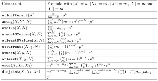
Table 1. Counting formulae extracted from range and roots reformulation Constraint Formula with|X| = n, |X1| = n1,|X2| = n2,|Y | = m and
|Y!| = m! alldifferent(X) m! (m−n)!· p n among(X, Y!, N ) !n N " m!N(m− m!)n−N· pn nvalue(X, N ) !mN"· an,N· pn atmostNValues(X, N ) #Nk=1!mk"an,k· pn atleastNValues(X, N ) #nk=N!m k " an,k· pn occurrence(X, y, N ) !Nn"(m− 1)n−N· pn atmost(X, y, N ) #Nk=1!nk"(m− 1)n−k· pn atleast(X, y, N ) #nk=N!n k " (m− 1)n−k· pn uses(X, X1, X2) mn−n1−n2·#mk=1 !m k " an1,kkn2· pn
disjoint(X, X1, X2) mn−n1−n2·#min(nk=1 1,m)#l=1min(n2,m−k)!mk"!m−kl "an1,kan2,l·
pn Proposition 12. Let N ∈ N, E (#occurrence(X, y, N)) = ,n N -(m − 1)n−N· pn (19)
Proof. The proof is the same as Proposition11in the case where Y" = {y} is a
singleton. '(
Proposition12can also be generalized to the case where N is a variable.
4.5 Synthesis
We report the estimators of the number of solutions in Table1 for several car-dinality constraints. We observe a pattern in all these formulae: the estimation of the number of allowed tuples is always pn multiplied by the number of tuples
allowed by the constraint if every domain were equal to the set of values Y (if the value graph were complete). This remark leads to the following Proposition. Proposition 13. Let C be a constraint over X with |X| = n, Y be the union of the domains and p the edge density in the value graph GX,Y, then:
E (#C) = #C∗· pn (20)
with #C∗ the number of allowed tuples if G
X,Y were complete.
Proof. Let SC∗ be the set of allowed tuples if GX,Y were complete. For each
s ∈ SC∗, let Zs be the random variable such that, Zs = 1 if s is in the set of
101 103 105 0 50 100 nb backtracks % solv ed maxSD ER maxSD PQZ dom/wdeg abs ibs 102 104 106 0 50 100 times (in ms) % solv ed
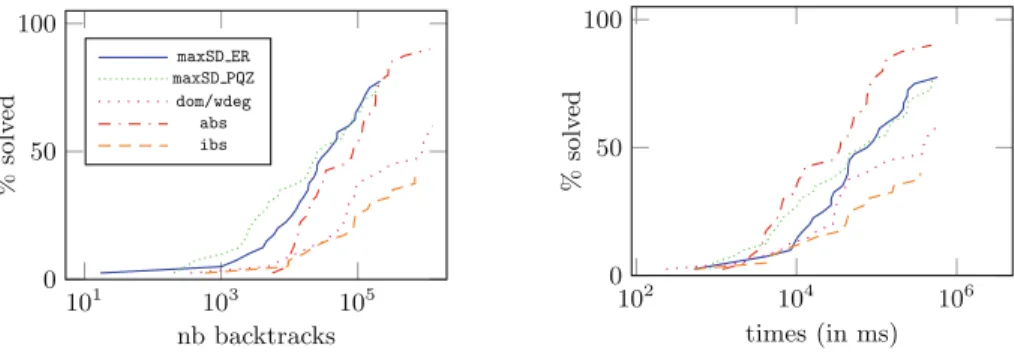
Fig. 2. Performances of maxSD ER, maxSD PQZ, dom/wdeg, ibs and abs on 40 hard Latin Square instances, in number of backtracks (left) and time (right).
of every variable, then, in the Erd˝os-Renyi Model, P ({Zs= 1}) = E (Zs) = pn.
Then, E (#C) = E $ s∈SC∗ Zs = $ s∈SC∗ E (Zs) = #C∗· pn ' ( In Sect.3, we have shown how to count solutions on a range and a roots constraints and in Sect.4, how to use the range and roots/decomposition to estimate the number of solutions on many cardinality constraints. Proposition13
highlights a general pattern for such estimates. In Sect.5, we experiment these probabilistic estimators within counting-based heuristics on some problems using cardinality constraints.
5
Experimental Analysis
In this section, we present two problems, on which we have run different heuris-tics: maxSD [13], dom/wdeg [3], abs (activity-based search) [10] and ibs (impact-based search) [15]. This benchmark has been chosen by taking the problems in XSCP, CSPLib, MiniZinc which matched our testing needs: no COP, with cardinality constraints at the core of the problem but no gcc. Also, the lack of knowledge on how to use maxSD on problems with several constraints restricts a lot the practical use of the heuristic. These conditions restricted our benchmark to Latin Squares and Sports Tournament Scheduling.
maxSDconsists in choosing a pair variable/value based on the estimation of the number of remaining solutions. More precisely, for each constraint, and for each pair variable/value in this constraint, we compute an estimation of the number of remaining allowed tuples and we associated with each pair a solu-tion density. maxSD chooses the pair variable/value that maximizes the solusolu-tion density among every constraint.
We actually do not run maxSD as presented in [13], but a slightly different version. It consists in re-computing the ordering of the variables only when the product of the domains size have decreased enough, as suggested in [6]. Here, we set a threshold at 20%. Also, the coefficients an,m, the binomial coefficients and
the factorials are computed in advance. The computation of the approximations is thus made in linear time in n.
We first introduce the problem and the cardinality constraints that are used in the model and then compare their efficiency in terms of solving time and number of required backtracks. The instances and the strategies are implemented in Choco solver [14] and we run them on a 2.2 GHz Intel Core i7 with 2.048 GB.
5.1 Latin Square Problem
A Latin Square problem is defined by a n ∗ n grid whose squares each contain an integer from 1 to n such that each integer appears exactly once per row and column [12]. The model uses a matrix of integer variables and an alldifferent constraint for each row and each column. We tested on the 40 hard instances used in [13] with n = 30 and 42% of holes (corresponding to the phase transition), generated following [7]. For these instances, we also compare our probabilistic estimator (maxSD ER) with the estimator that is proposed in [13] (maxSD PQZ) for alldifferent. We set a time limit to 10 min.
Figures2 represent the percentage of solved instances in function of the number of required backtracks, and of the solving time. The strategies maxSD (for both estimators maxSD ER and maxSD PQZ) and abs performed better than dom/wdeg and ibs. abs solved more instances than the two versions of maxSD, but required more backtracks. maxSD seems to perform better on the easiest instances (in term of number of backtracks). maxSD PQZ has slightly better per-formances than maxSD ER on the medium instances and have very comparable performances on the hardest ones.
5.2 Sports Tournament Scheduling Problem
This problem is taken from [19] and is presented as follows: the problem is to schedule a tournament of n teams over n − 1 weeks, with each week divided into n/2 periods, and each period divided into two slots. A tournament must satisfy the following three constraints: every team plays once a week; every team plays at most twice in the same period over the tournament; every team plays every other team. The first and the third constraint are modeled with an alldifferent constraint and the second one is modeled with an atmost constraints. We run this problem with the different settings: n ∈ {6, 8, 10, 12, 14}.
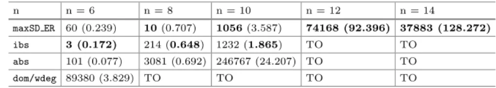
In Table 2, we report the number of backtracks required (and the time required) to solve the problem for different values of n with four different heuris-tics. Here maxSD PQZ cannot be used as there is no estimator for atmost in the previous work of [13]. Consequently, we only focused on our approach maxSD ER. We fixed a time limit to 5 min. We observe that maxSD ER outperforms abs and
dom/wdeg. For n ∈ {6, 8, 10}, maxSD ER and ibs have similar performances but ibscould not find a solution in less than 5 min for n = 12 and n = 14.
Table 2. Number of backtracks (time in s) for different settings of n
n n = 6 n = 8 n = 10 n = 12 n = 14
maxSD ER 60 (0.239) 10 (0.707) 1056 (3.587) 74168 (92.396) 37883 (128.272) ibs 3 (0.172) 214 (0.648) 1232 (1.865) TO TO
abs 101 (0.077) 3081 (0.692) 246767 (24.207) TO TO
dom/wdeg 89380 (3.829) TO TO TO TO
We have shown that our probabilistic estimator for alldifferent gives very comparable result than the estimator given in [13] on the Latin Square instances. Also our estimators within maxSD ER gives better results than ibs, abs and dom/wdegon the Sport Tournament Scheduling problem.
6
Conclusion
In this paper, we have presented a method to estimate the number of solutions of the range and roots constraints with a probabilistic Erd˝os-Renyi Model. We can estimate the number of solutions of ten cardinality constraints using their range and roots decompositions. We detailed our method on alldifferent, nvalue, among and occurrence and we report our estimators with atmostNValues, atleastNValues, atmost, atleast, uses and disjoint. We highlighted a gen-eral formula to compute such an estimation on cardinality constraints. We have implemented the heuristic maxSD ER with these new probabilistic estimators and compare their efficiency to dom/wdeg, abs, and ibs.
We think that the main asset of this approach is its systematic nature. We have shown here an application of counting solutions for counting based search. Such an approach could also be used, for example, for uniform random instances generation, probabilistic reasoning or search space structure analysis.
We did not study the gcc constraint in this article, as its decomposition involves several non-disjoint subsets of the variables. Further research includes extending our approach to the case where several range and roots constraints may apply to a common set of variables. This will lead us to estimators of the number of solutions for conjunctions of cardinality constraints, or gcc con-straints.
References
1. Beldiceanu, N., Contejean, E.: Introducing global constraints in chip. Math. Com-put. Modell. 20(12), 97–123 (1994). https://doi.org/10.1016/0895-7177(94)90127-9.http://www.sciencedirect.com/science/article/pii/0895717794901279
2. Bessiere, C., Hebrard, E., Hnich, B., Kiziltan, Z., Walsh, T.: Range and roots: two common patterns for specifying and propagating counting and occurrence con-straints. Artif. Intell. 173(11), 1054–1078 (2009).https://doi.org/10.1016/j.artint. 2009.03.001
3. Boussemart, F., Hemery, F., Lecoutre, C., Sais, L.: Boosting systematic search by weighting constraints. In: de M´antaras, R.L., Saitta, L. (eds.) Proceedings of the 16th European Conference on Artificial Intelligence, ECAI 2004, Including Prestigious Applicants of Intelligent Systems, PAIS 2004, Valencia, Spain, 22–27 August 2004, pp. 146–150. IOS Press (2004)
4. Carlsson, M., Fruehwirth, T.: Sicstus PROLOG user’s manual 4.3. Books On Demand - Proquest (2014)
5. Erdos, P., Renyi, A.: On random matrices. Publication of the Mathematical Insti-tute of the Hungarian Academy of Science (1963)
6. Gagnon, S., Pesant, G.: Accelerating counting-based search. In: van Hoeve, W.-J. (ed.) CPAIOR 2018. LNCS, vol. 10848, pp. 245–253. Springer, Cham (2018).
https://doi.org/10.1007/978-3-319-93031-2 17
7. Gomes, C., Shmoys, D.: Completing quasigroups or latin squares: a structured graph coloring problem, January 2002
8. Gomes, C.P., Hoffmann, J., Sabharwal, A., Selman, B.: From sampling to model counting. In: Proceedings of the 20th International Joint Conference on Artificial Intelligence, IJCAI 2007, Hyderabad, India, 6–12 January 2007, pp. 2293–2299 (2007)
9. Meel, K.S., et al.: Constrained sampling and counting: universal hashing meets SAT solving. CoRR abs/1512.06633 (2015).http://arxiv.org/abs/1512.06633
10. Michel, L., Van Hentenryck, P.: Activity-based search for black-box constraint programming solvers. In: Beldiceanu, N., Jussien, N., Pinson, ´E. (eds.) CPAIOR 2012. LNCS, vol. 7298, pp. 228–243. Springer, Heidelberg (2012).https://doi.org/ 10.1007/978-3-642-29828-8 15
11. Pachet, F., Roy, P.: Automatic generation of music programs. In: Jaffar, J. (ed.) CP 1999. LNCS, vol. 1713, pp. 331–345. Springer, Heidelberg (1999).https://doi. org/10.1007/978-3-540-48085-3 24
12. Pesant, G.: CSPLib problem 067: quasigroup completion.http://www.csplib.org/ Problems/prob067
13. Pesant, G., Quimper, C., Zanarini, A.: Counting-based search: branching heuris-tics for constraint satisfaction problems. J. Artif. Intell. Res. 43, 173–210 (2012).
https://doi.org/10.1613/jair.3463
14. Prud’homme, C., Fages, J.G., Lorca, X.: Choco solver documentation. TASC, INRIA Rennes, LINA CNRS UMR 6241, COSLING S.A.S. (2016). http://www. choco-solver.org
15. Refalo, P.: Impact-based search strategies for constraint programming. In: Wallace, M. (ed.) CP 2004. LNCS, vol. 3258, pp. 557–571. Springer, Heidelberg (2004).
https://doi.org/10.1007/978-3-540-30201-8 41
16. R´egin, J.: A filtering algorithm for constraints of difference in CSPS, pp. 362–367 (1994)
17. Russell, S.J., Norvig, P.: Artificial Intelligence - A Modern Approach, 3rd edn. Pearson Education, London (2010).http://vig.pearsoned.com/store/home/1,1205, store-14563 id-294438,00.html
18. Stanley, R.P.: Enumerative Combinatorics: Volume 1, 2nd edn. Cambridge Uni-versity Press, Cambridge (2011)
19. Walsh, T.: CSPLib problem 026: sports tournament scheduling.http://www.csplib. org/Problems/prob026