HAL Id: hal-02309458
https://hal.archives-ouvertes.fr/hal-02309458
Submitted on 9 Oct 2019HAL is a multi-disciplinary open access
archive for the deposit and dissemination of sci-entific research documents, whether they are pub-lished or not. The documents may come from teaching and research institutions in France or abroad, or from public or private research centers.
L’archive ouverte pluridisciplinaire HAL, est destinée au dépôt et à la diffusion de documents scientifiques de niveau recherche, publiés ou non, émanant des établissements d’enseignement et de recherche français ou étrangers, des laboratoires publics ou privés.
The Guttman errors as a tool for response shift
detection at subgroup and item levels
Véronique Sébille, Alice Guilleux, Jean-Benoit Hardouin, Myriam Blanchin
To cite this version:
Véronique Sébille, Alice Guilleux, Jean-Benoit Hardouin, Myriam Blanchin. The Guttman errors as a tool for response shift detection at subgroup and item levels. Quality of Life Research, Springer Verlag, 2016, 25 (6), pp.1385-1393. �10.1007/s11136-016-1268-8�. �hal-02309458�
1
The Guttman errors as a tool for response shift detection at subgroup
and item levels
Myriam Blanchin1*, Véronique Sébille1, Alice Guilleux1, Jean-Benoit Hardouin1
1 EA 4275, Biostatistics, Pharmacoepidemiology and Subjective Measures in Health Sciences, University of Nantes, France
*Correspondence to: Myriam Blanchin
2
Abstract
Purpose
Statistical methods for identifying response shift (RS) at the individual level could be of great practical value in interpreting change in PRO data. Guttman errors (GE) may help to identify discrepancies in respondent’s answers to items compared to an expected response pattern and to identify subgroups of patients that are more likely to present response shift. This study explores the benefits of using a GE based method for RS detection at the subgroup and item levels.
Methods
The analysis was performed on the SatisQoL study. The number of GE was determined for each individual at each time of measurement (at baseline T0 and 6 months after discharge M6). Individuals showing discrepancies (with many GE) were suspected to interpret the items differently from the majority of the sample. Patients having a large number of GE at M6 only and not at T0 were assumed to present RS. Patients having a small number of GE at T0 and M6 were assumed to present no RS. The RespOnse Shift Algorithm in Item response theory (ROSALI) was then applied on the whole sample and on both groups.
Results
Different types of RS (non-uniform recalibration, reprioritization) were more prevalent in the group composed of patients assumed to present RS based on GE. On the opposite, no RS was detected on patients having few GE.
Conclusions
Guttman errors and Item Response Theory models seem to be relevant tools to discriminate individuals affected by RS from the others at the item level.
Keywords
3
Introduction
Patient-Reported Outcomes (PRO) are increasingly used in longitudinal studies to take into account patient’s perspective and experience of disease and assess perceived health changes over time. The interpretability of PRO data and of its evolution can be complex and obfuscated by several phenomena, such as response shift (RS) due to the patients’ changing standards, values, or conceptualization of what the PRO is intended to measure. As a consequence of RS, observed patient’s changes may reflect true perceived health changes combined with questionnaire perception changes. RS can also be viewed as an indication of a possible therapeutic benefit coming from some form of psychological adaptation or adjustment. It has been hypothesized that RS can result from three different processes: i) recalibration (changes in the patient’s internal standards of measurements), ii) reprioritization (changes in the patient’s values), and iii) reconceptualization (changes in the patient’s definition of what is being measured) [1]. Several approaches have been proposed for RS detection and adjustment in the appraisal of change of PRO over time such as the “then-test” [1], Structural Equation Modeling (SEM) [2], Item Response Theory (IRT) [3], or group-based trajectory analysis (latent trajectories created from the centered residuals of a random effects model to identify subgroups of the population) [4]. Among these, the “then-test” only allows for the detection of recalibration RS while SEM and IRT allow for all types of RS detection (recalibration, reprioritization and reconceptualization), even though it seems that IRT has to date only been applied for recalibration and reprioritization RS. In contrast, group-based trajectory analysis will indicate that RS is suspected and will not allow for determining the type of RS that occurred but can give clues to the timing of RS.
Further, the “then-test” as well as the SEM and IRT approaches allow for the detection of RS at the group level, while group-based trajectory analysis can be used for identifying RS at the individual level. It has already been discussed [4] that statistical methods for identifying RS at the individual level could be of great practical value in interpreting change in PRO data. In fact, group level based analyses may mask important meaningful differences over time.
4
Moreover, in order to gain more insight on the RS phenomena, RS detection at the item level could also be worthwhile investigating. Following these ideas, it might be of value to propose a method for RS detection at the individual and item levels also allowing for the identification of the different types of RS. Using IRT models could be interesting because they are formulated at item level. In the IRT framework, RS detection is based on item parameters such as their difficulties and their discrimination power. When no RS is assumed, item parameters are not supposed to vary over time. RS is suspected otherwise.
To go towards RS detection at a more individual level, we propose a method to detect RS at subgroup level. To further assess whether response patterns vary at an individual level, indices such as the number of Guttman errors [5] may be used to detect discrepancies in respondent’s answers compared to an expected response pattern under some hypothesis (no RS for instance). Discrepancies and resulting Guttman errors at each time of measurement may help identifying patients that might perceive the questionnaire differently than the majority of the sample over time (assumed to not present RS). Such an approach could identify subgroups of patients that are more likely to present response shift.
The aim of this study was to explore the benefits of using a new method combining IRT and Guttman errors for RS detection across subpopulations at item level for estimating and interpreting observed differences in quality of life over time in a clinical study.
Material and Methods
Sample
This analysis was performed on a subsample of the SatisQoL study [6]. The SatisQoL study is a French multicenter (3 centers) cohort study designed to assess the relationships between satisfaction with care and Health-Related Quality of Life (HRQL) after being hospitalized in a university hospital for a medical or surgical intervention related to a chronic disease. Patients between 18 and 75 years old, suffering from a chronic disease for less than 6 months at initial admission, and undergoing a medical or surgical intervention during
5
hospitalization could be enrolled in the study. Patients were asked to fill in a variety of questionnaires (including HRQL measurement) shortly after admission (T0), and at 6 months after discharge (M6). In this study, we focused on patients who underwent surgery.
Main outcome
HRQL was assessed at baseline and 6 months after discharge using the SF36 v1.3 in French [7] [8]. This analysis was restricted to the General Health (GH) dimension of the SF-36 composed of 5 items having 5 answer categories (Excellent/ Very good/ Good/Fair/ Poor or Definitely true/ Mostly true/ Don’t know/ Mostly false/ Definitely false): (i) item 1 “In general, would you say your health is”, (ii) item 33 “I seem to get sick a little easier than other people”, (iii) item 34 “I am as healthy as anybody I know”, (iv) item 35 “I expect my health to get worse” and (v) item 36 “My health is excellent".
Identification of individuals with discrepancies
In a first step, individuals with observed discrepancies based on the number of Guttman errors [5] at each time of measurements were identified and assigned in different groups. Guttman errors are simple to implement as no parameters need to be estimated. It only requires the rank-ordering of the response categories and the assumption that an individual perceiving the items in the same manner than the majority of the sample and answering positively to a given response category to an item will also answer positively to easier response categories (that have a lower rank). Following this assumption, Guttman errors represent the total number of incoherent combinations of responses between all the combinations of two items for each patient. They were computed by ordering all the possible response categories (of all of the answered items) from the easiest (the most prevalent) to the most difficult (the least prevalent). A Guttman error was identified as soon as a patient responded to a given response category for one item of the questionnaire and simultaneously did not respond to an easier response category to another item. In this work, the response categories are ordered using the patients’ responses observed at the first time
6
of measurement (T0 in the whole sample). The number of Guttman errors was subsequently determined for each individual at each time of measurement (T0 and M6). To determine the number of Guttman errors that define a low or high number of Guttman errors, we looked at the two histograms of the Guttman errors at times T0 and M6 respectively. A cut off was graphically determined using the distribution of individuals’ number of Guttman errors in order to distinguish at each time of measurement patients with a lot of Guttman errors from the others.
Four groups of patients were subsequently defined given that they presented a lower number of Guttman errors than the cut off or not at a given time. Patients showing a small number of Guttman errors at T0 and at M6 were assumed to have the same perception of the questionnaire over time and to present no RS and were allocated in the “No discrepancy” group. The “Late discrepancies” group is composed of patients having a large number of Guttman errors at M6 only and not at T0. Hence, it corresponds to patients having the same perception of the items as the majority of the sample at T0 but a different perception at M6 which could fit with the usual definition of response shift.
The other two groups contain patients having discrepancies at T0 and could be composed of various types of discrepancies including response shift or differential item functioning (DIF) for instance. The “Early discrepancies” group is composed of patients having a large number of Guttman errors at T0 only but not at M6. The patients having a large number of Guttman errors at T0 and at M6 belong to the “Persistent discrepancies” group which could correspond to a group of patients presenting differential item functioning and other deviations from the response pattern of the majority of the sample.
Detection of the response shift
In a second step, the RespOnse Shift Algorithm in Item response theory (ROSALI) [3] was applied on the whole sample of patients and on the “No discrepancy” and “Late discrepancies” group separately. Patients in the “No discrepancy” group were assumed to present no RS given the clustering and we expected no or few response shifts detected with
7
ROSALI in this group. On the opposite, patients in the “Late discrepancies” group were assumed to fit with the usual definition of response shift given the clustering and we expected to detect different types of response shift with ROSALI in this group. The “early discrepancies” and “persistent discrepancies” seem to be composed of various sources of deviations and the use of ROSALI would probably not be adequate in these groups. Therefore, ROSALI was not applied on the “early discrepancies” and “persistent discrepancies” groups.
ROSALI is an algorithm for RS detection at item level using IRT polytomous models, the longitudinal generalized partial credit model and the longitudinal partial credit model. This algorithm allows non-uniform and uniform recalibration, reprioritization detection and true change estimation with these types of RS taken into consideration if appropriate. ROSALI detects and takes account of response shift following different steps:
0. Estimating the item difficulties from the data at T0 in a preliminary step
1. Establishing a measurement model (Model 1) taking into account the following types of RS: recalibration (uniform and non-uniform) and reprioritization (step 1). The measurement model assumes no true change.
2. Fitting a model with true change and no RS (model 2) and evaluating overall RS by a LR test comparing model 1 and model 2 (step 2).
3. If the LR test is significant (overall RS detected): Detecting each type of RS on each item (step 3) by releasing constraints on RS parameters one at a time starting from model 2. Each release of constraint is tested by likelihood ratio tests and the most significant is retained to update the model (model 3). The model 3 is updated iteratively until no more RS is detected. All tests for response shift detection are adjusted using Bonferroni correction for multiple comparisons.
The RS is hierarchically detected as items presenting recalibration are identified first. At the same time, the type of recalibration (uniform or non-uniform) is determined. Then, items presenting reprioritization are identified.
8
4. Estimating true change (step 4) in a model accounting for all types of response shifts detected in the previous steps (model 4).
The statistical analyses were performed with Stata 13 MP and SAS 9.3.
Results
Sample characteristics
Table 1 summarizes characteristics of the 669 patients who underwent surgery included in this study (Selected sample – SS). The average age was 55 years old, 53% of the patients were men and 16% lived alone. They had, in average, 2.1 children and 32% of the patients had a professional activity. The 669 patients went through various surgical procedures belonging to 11 medical areas.
Among these patients, 29 (4%), 118 (18%) and 23 (3%) did not completely fulfill the items related to GH dimension of the SF36 questionnaire at T0, M6 or T0 and M6 respectively. Consequently the Guttman errors of each patient could be computed for only 499 patients at the two times of measurement (Work sample – WS). The histograms (data not shown) at times T0 and M6 of the Guttman errors presented a bimodal distribution with a cutoff at about 5 errors. Four groups of patients were subsequently defined:
No discrepancy group: individuals with less than 5 Guttman errors at T0 and at M6 Late discrepancies group: individuals with less than 5 Guttman errors at T0 and at
least 5 at M6
Early discrepancies group: individuals with at least 5 Guttman errors at T0 and less than 5 at M6
Persistent discrepancies group: individuals with at least 5 Guttman errors at T0 and at M6.
9
Table 1 presents a descriptive analysis of the 4 groups of patients. There were significant differences between the 4 groups in terms of age (p=0.03), with lower age for the group with persistent discrepancies, and a difference close to significance for the number of children (p=0.07). There were no significant differences in terms of sex (p=0.74), familial status (p=0.45), level of education (p=0.62), professional activity (p=0.28), reason for hospital admission (p=0.44), and hospitalization duration (p=0.86).
Response shift detection
Table 2 describes for the work sample and for each group with no discrepancies at T0 the types of response shift detected using ROSALI. In the work sample, reprioritization is detected on the items 33 to 36. In the group with no discrepancies, no type of response shift is detected. Many types of response shift are detected in the group with late discrepancies. All five items of the GH scale are affected by RS. Indeed, items 33, 34, 35 and 36 are affected by reprioritization and items 1, 33, 34 and 35 are also affected by non-uniform recalibration in this group. The same items are affected by reprioritization in the work sample and in the “Late discrepancies” group but they are not affected in the same way. In the work sample, items 34 and 36 are more predictive of the latent trait level (RP parameter estimates>1) at M6 than at T0. On the opposite, items 33 and 35 are less predictive of the latent trait level at M6 than at T0. In the “Late discrepancies” group, items 33, 34, 35 and 36 are all less predictive of the latent trait level at M6 than at T0.
Place Table 2 approximately here.
In the “Late discrepancies” group, the non-uniform recalibration affecting the item 1 “In general, would you say your health is “ results in a narrower distribution of the item difficulties along the latent trait continuum at M6 compared to T0. Indeed, the two most difficult item difficulties become easier at M6 and inversely, the two easiest item difficulties become more difficult at M6. For the same level of latent trait at both times of measurement, it is more
10
difficult to endorse “fair” rather than “poor“ and “good” rather than “fair” categories at M6 and it is easier to endorse “very good” rather than “good“ and “excellent” rather than “very good” categories at M6 (item 1 is reversed for the analysis). For items 33, 34 and 35, three out of four item difficulties become easier at M6, including the easiest and the most difficult item difficulties of each item, leading to a global shift to the left of the latent trait continuum due to non-uniform recalibration. Recalibration is non-uniform because 1 over 4 item difficulties shift in the other way (on the right of the latent trait continuum) for each of the items 33, 34 and 35 and the shifts of the item difficulties for a given item have not the same magnitude.
Place Table 3 approximately here.
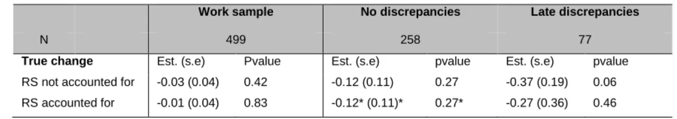
Table 3 presents the estimates of the true change parameter and its standard error in models accounting for RS or not. In the work sample and in the group with no discrepancies, no significant change is observed between T0 and M6 whether the RS is accounted for or not. In the group with late discrepancies, the change is higher when the RS is not accounted for and the estimated change between T0 and M6 is almost significant (p=0.06). When the RS is taken into account in the model, the estimated change decreases of 0.10 and is not significantly different from 0 (p=0.46).
Discussion
This paper presents the response shift detection on the GH dimension of the SF-36 questionnaire at two times of measurement (at the end of hospitalization (T0) and 6 months later (M6)) on a subsample of the SatisQoL study using two different ways of handling response shift between these two times of measurement. A model considering response shift at the sample level (work sample) is compared to a model where the response shift is detected in 2 groups dividing individuals assuming to present response shift or not based on their individual number of Guttman errors.
11
As expected, types and amount of detected RS differ in the work sample and in the two groups. Reprioritization was found on four items in the work sample. In the “no discrepancies” group, no response shift was detected. The absence of response shift in the “no discrepancies” group compared to the work sample is in agreement with the assumption that the patients with few Guttman errors at T0 and M6 are supposed to present no or less RS than the remainder of the sample. On the opposite, in the “late discrepancies” group, non-uniform recalibration affected four items and reprioritization was found on four items. This group was composed of patients with few Guttman errors at T0 and many Guttman errors at M6 and so assuming to present RS at M6 following the usual definition of response shift where a change in the standards or values of patients is assumed to have occurred between the two times of measurement. Therefore, the large amount of RS detected in this group seems consistent with the clustering based on Guttman errors.
Furthermore, this study has also shown that the estimation of the true change can vary a lot whether the response shift is taken into account or not in the different groups identified according to the number of Guttman errors. In the work sample where a small amount of RS was detected, the estimated true change was not significantly different from 0 whether the response shift was taken into account or not. But, in the “late discrepancies” group, where all items were affected by different types of RS, the estimated true change is higher when RS is not accounted for and almost leads to conclude to a deterioration of the health related quality of life on the global health dimension between T0 and M6 (p=0.06). When RS is accounted for, the estimation of the true change is not significant and shows that the global health has stayed stable between T0 and M6 for the “late discrepancies” group (p=0.46).
ROSALI has been previously applied on the SatisQoL dataset [3]. Results in terms of response shifts in the ROSALI paper are quite different from the results of the work sample in this study. In the ROSALI paper, non-uniform recalibration was found on item 1 and uniform recalibration was found on item 35 for IRT. Reprioritization was evidenced on all items of the
12
GH subscale. In the work sample, reprioritization was detected on items 33, 34, 35 and 36 and no recalibration was detected. Guttman errors can only be computed if the patients answered all items at both times of measurement. Consequently, 79 patients (13.7%) of the sample included in the ROSALI paper (N=578) are not included in the work sample (N=499). Therefore, missing data seems to have an impact on the results of response shift detection. As well as other methods for response shift detection that are quite new, the performance of the ROSALI algorithm has to be assessed through simulation studies. Simulation studies would allow validating the whole procedure to detect response shift by assessing whether the different steps correctly detect the correct type of response shift on the correct items, in case of complete or incomplete data. Such studies would also help to quantify the potential bias in parameter estimates and evaluate the impact of missing data on the response shift detection. Finally, the separate response shift detection analyses in each group and in the work sample led to set the item parameters at T0 to different values for each group. In fact, the item parameters were automatically set to the estimated values estimated in the step 0 of ROSALI within each group. A more refined way to proceed to the response shift detection would be to set the item parameters within each group to the estimated values of the work sample to make the comparisons between each group and the work sample more sensible. In practice, the ROSALI algorithm package has not been developed with this option and this will be an important development for the future.
From a methodological point of view, this approach raises several questions. First, the choice of the reference frame (T0) to determine the order of the response categories and consequently the number of Guttman errors to identify individuals presenting discrepancies at T0 or M6 can be questioned. Then, the threshold for the number of Guttman errors (set to 5 in this analysis) to determine the groups that should be further explored in a sensitivity analysis as this cutoff can lead to more or less homogeneous groups. Furthermore, this threshold should be higher than the number of Guttman errors due to chance to ensure a meaningful clustering. In this context, the choice of the questionnaire has its importance as a
13
questionnaire validated with IRT might produce less Guttman errors by chance and thus allows a better identification of individuals with discrepancies or not. A good way to improve the clustering of patients could be to define the groups by recursively partitioning the Guttman errors at T0 and T6 following the idea of the GetR package [9]. In this approach, the Guttman error tree constructed by recursive partitioning is adapted for cross-sectional designs. A Guttman error tree adapted to a longitudinal design could possibly define more homogeneous subgroups and overcome the difficulties related to the determination of the threshold. Another limit is related to the way the discrepancies were considered at each time, in a binary fashion (presence/absence) in this analysis. It could be of value to link the number of Guttman errors per patient with more than one threshold to define the subsequent groups more precisely and in a more homogeneous way. However, this would imply a greater number of groups of patients, thus increasing the complexity of the analyses and requiring large sample sizes. Finally, other indices could be considered to identify individuals presenting discrepancies. Stochastic non-parametric IRT-models has a long-standing tradition of using statistical methods to identify aberrant response patterns [10, 11], but most of these have been applied in educational research and/or to dichotomous items only. PRO studies are structurally different from studies in educational and psychological measurements because the number of individuals and the number of items are small compared to studies in educational measurement. The performance of the Guttman error based indices seems to have never been evaluated in the context of PRO studies. Another main difference is that PRO questionnaires are mainly composed of polytomous items. The items are not easily convertible from polytomous to dichotomous items and it is generally out of purpose to dichotomize them as a lot of information might be lost and this may distort the validity and reliability of the PRO questionnaires. Other statistical methods could provide an index with higher performance (based on indices derived from Guttman errors or on CUSUM for example) to detect deviations from an expected response pattern than the number of Guttman errors but further research on their applicability is warranted.
14
The “classify-analyze” strategy implemented in this study is a natural stepwise approach [12] but pitfalls of this strategy have been documented in the latent class analysis and general growth mixture modeling literature [13]. For instance, a study [14] where subgroups are created first, by fitting a latent class growth mixture to distinguish a number of life satisfaction trajectories, and where presence of response shift is determined thereafter, by comparative analyses between life satisfaction measures in each of the subgroups, may lead to biased parameter estimates in the second step [15]. In this example, the second step (analysis step) assumes that all cases are perfectly assigned to a class and ignores the fact that a case could be not assigned to the correct class. The uncertainty in the class membership of the classification step has to be integrated in the secondary analysis to avoid biases results. Our study follows a “classify-analyze” strategy and results might suffer from this two-step approach. Contrary to the growth mixture modeling, the definition of groups based on Guttman errors does not bring uncertainty in class membership as the number of Guttman errors are deterministically computed from the rank-ordering of the response categories. But, the uncertainty related to the rank-ordering of the response categories based on the observed responses of the patients probably has an effect on the results of the response shift detection in the subgroups. Several research paths have to be investigated to evaluate the performance of the proposed approach and to improve it regarding its deterministic aspect in the first step (Guttman errors). Firstly, its performance and the potential bias on the results could be evaluated in a simulation study. Then, some recent developments regarding the “classify-analyze” strategy could help to improve the results obtained for the response shift detection step. Two approaches have proven to perform well to take into account the classification error: the step approach and the three-step approaches [15,16,17]. A one-step approach seems attractive but complicated to implement in our case. This would lead to consider a longitudinal mixture IRT model [18] or an adaptation of the overlapping waves model [19] to allow defining different latent trajectories and simultaneously defining different item response patterns. Since complex growth mixture models and complex IRT models both have convergence problems, we can hypothesize that such a model, no matter how
15
attractive it might be, might fail to converge or that the estimation process may take a considerable time using maximum likelihood estimation. As mixture IRT models have been developed in educational measurement, their performances have been evaluated with large item sample sizes (60 to 240 items in [18]) and large person sample sizes (350 to 700 individuals in [18]). The common small number of items and of individuals in PRO studies compared to educational measurement studies raise the question of the performance of mixture IRT models in this context. Recent developments in Bayesian estimation of both growth mixture [20] and IRT models [21] could fasten the estimation process but might not solve the problem of small sample sizes in PRO studies. A Bayesian estimation of the parameters will also lead to redevelop ROSALI that was based on maximum likelihood estimation and to determine the appropriate a priori distribution of the parameters for which little is known. Apart from these technical considerations, interpretation of such models will be very difficult as each individual could have a different trajectory as well as a different growth. A clear identification of the presence of response shift and of the type of response shift will probably be difficult. However, it is clear that these models have the advantage of detecting response shift at the individual level rather than at the subgroup level and allow including covariates to describe differences between the classes.
Another adaptation could be to take account of the uncertainty of the first step in the response shift detection step such as in the three-step approach [16,17]. In the mixture modeling domain, a step is added between the classification step and the secondary analysis to compute weights to be used in the secondary analysis that will correct the bias due to the uncertainty of class membership. Developing a three-step approach for response shift detection at subgroup level assumes that we would be able to quantify analytically the potential bias due to the clustering based on Guttman errors. As for a one-step approach, a three-step approach would not be straightforward and will require extended developments.
Regarding the clinical implication of this work, we only consider patients having a surgical intervention in the SatisQoL dataset (669 patients among the 1473 patients of this study –
16
45%). By doing so, we tried to select patients that could be more likely to present response shift (since a catalyst is assumed to be required in order to present response shift [22, 23]). It can be hypothesized that results might have been different using the whole sample of the SatisQoL study. Furthermore, selecting patients who underwent surgery led to consider a very heterogeneous group of patients in term of disease and type of surgery. This might explain the fact that a large number of patients of the sample (about 33%) had a lot of Guttman errors at T0.
The interpretation of the link between discrepancies measured using Guttman errors and response shift can also be questioned. The detection of response shift could not be adequate on the two groups with discrepancies at T0, the “early discrepancies” and the “persistent discrepancies” groups. In the usual definition of response shift at sample level, the time of reference is T0 and all the individuals are assumed to display the same amount and types of response shift at M6 compared to T0. By looking at the subgroup level, Guttman errors identified patients whose perception of the questionnaire is already different from the whole sample at T0. The “early discrepancies” group presents few Guttman errors at M6 so we can assume that the perception of the questionnaire is then becoming similar to the majority of the sample. But we can wonder if this evolution can be considered as a response shift in its usual definition. Furthermore, the “persistent discrepancies” group presents also many Guttman errors at M6 but these discrepancies may not necessarily be on the same items between T0 and M6. Hence, this group may be composed of patients whose discrepancies are not on the same items at both times of measurement and for whom response shift detection and interpretation makes sense. But, this group can also contain patients whose discrepancies are on the same items at both times and these patients should rather be considered as having no response shift. As these patients have a different perception of the questionnaire compared to the whole sample at both times of measurement, differential item functioning [24, 25] may occur if the discrepancies pertain to the same items over time for this subsample. So, the “persistent discrepancies” group may mix together very different
17
patients and response shift detection assuming that all the patients of this group are affected the same way seems not adequate. The clustering of patients based on Guttman errors has to be improved to include not only the number of Guttman errors but also the items with discrepancies at each time of measurement. The identification of patients with persistent discrepancies on the same items over time or not might help to better assign patients in the “persistent discrepancies” group and to perform response shift detection wisely. The idea that patients might show various types of deviations in the groups with discrepancies at T0 is supported by the results obtained trying to apply ROSALI on these groups. For both groups, convergence problems appeared in steps 1 and 2 of ROSALI when fitting a model without true change and RS accounted for (Model 1) or when fitting a model with true change and RS not accounted for (Model 2). As a reminder, in the preliminary step of ROSALI, item difficulties are estimated at T0 and these values are then used in longitudinal models 1 and 2 to set the values of the item difficulties. As both groups present many Guttman errors at T0, patients might be very heterogeneous and item difficulties in the preliminary step might be misestimated. Hence, models 1 and 2 may be difficult to fit because item difficulties were potentially set to erroneous values. Selecting patients with a high number of Guttman errors at T0 might lead to combine together deviations due to response shift, to DIF and to violations of the model. Therefore, a parametric IRT model as models used in ROSALI might be unlikely to fit whereas patients have been selected due to their nonfitting to non parametric IRT (Guttman errors).
The “no discrepancies” group is composed of half of the patients of the sample and each of the three groups with discrepancies at T0 and/or M6 is composed of about a sixth of the patients. This distribution of the patients in the four groups argues in favor of response shift detection at the individual level in the future as it seems difficult to assume that all patients experience the same amount and the same type of response shift in the SatisQoL data. Therefore, mixing an item-level approach and an individual approach of the response shift phenomenon seems to be an interesting path of development for the analysis of subjective
18
concepts such as Patient-Reported Outcomes in a longitudinal framework. However, the best approach remains today unknown, and only methodological works through simulation studies for example will help determining advantages and drawbacks of the different approaches.
Acknowledgements
The authors gratefully acknowledge Frans J. Oort, Mirjam A.G. Sprangers and Mathilde G.E. Verdam for their comments on the manuscript.
This study was supported by the Institut National du Cancer, under reference “INCA_6931”. The SatisQoL cohort project (Investigators: P Auquier, F Guillemin (PI), M Mercier) was supported by an IRESP (Institut de recherche en santé publique) grant from Inserm, and a PHRC (Programme Hospitalier de Recherche Clinique) national grant from French Ministry of Health, France.
Compliance with ethical standards
Authors declare that they have no conflict of interest. All procedures performed in studies involving human participants were in accordance with the ethical standards of the institutional and/or national research committee and with the 1964 Helsinki declaration and its later amendments or comparable ethical standards. The SatisQoL study was approved by the national Institutional Review Board and the national committee for data protection (CCTIRS 07.212 and CNIL 1248560).
Bibliography
1. Schwartz, C. E. & Sprangers, M. A. (1999). Methodological approaches for assessing
response shift in longitudinal health related quality-of-life research. Social Science &
19
2. Oort, F. J. (2005). Using structural equation modeling to detect response shifts and
true change. Quality of Life Research, 14(3), 587–598.
3. Guilleux, A., Blanchin, M., Vanier, A., Guillemin, F., Falissard, B., Hardouin, J.B., Sébille,
V. (2015). RespOnse Shift ALgorithm in Item response theory (ROSALI) for response
shift detection with missing data in longitudinal patient-reported outcome studies.
Quality of Life Research, 24(3):553-564.
4. Mayo, N. E., Scott, S. C., Dendukuri, N., Ahmed, S. & Wood-Dauphinee, S. (2008).
Identifying response shift statistically at the individual level. Quality of Life Research,
17(4), 627–639. doi:10.1007/s11136-008-9329-2.
5. Sijtsma, K. & Molenaar, I. W. (2002). Introduction to Nonparametric Item Response
Theory, Vol. 5 (1st ed.). Sage Publications, Inc.
6. Kepka, S., Baumann, C., Anota, A., Buron, G., Spitz, E., Auquier, P. & Mercier, M. (2013).
The relationship between traits optimism and anxiety and health-related quality of life
in patients hospitalized for chronic diseases: data from the SATISQOL study. Health and
Quality of Life Outcomes, 11(1), 134. doi:10.1186/1477-7525-11-134.
7. Ware, J. E. & Sherbourne, C. D. (1992). The MOS 36-item short-form health survey
(SF-36). I. Conceptual framework and item selection. Medical Care, 30(6), 473–483.
8. Leplège, A., Ecosse, E., Verdier, A. & Perneger, T. V. (1998). The French SF-36 Health
Survey: translation, cultural adaptation and preliminary psychometric evaluation.
Journal of Clinical Epidemiology, 51(11), 1013–23. doi:9817119.
9. Beller, J., & Kliem, S. (2013). GetR: Calculate Guttman error trees in R (Version 0.1)
[Computer software]. Hannover, Germany. Retrieved from
http://cran.r-project.org/web/packages/GetR/
20
10. Meijer, R. R. (1994). The Number of Guttman Errors as a Simple and Powerful
Person-Fit Statistic. Applied Psychological Measurement, 18(4), 311‑314.
11. Tendeiro, J. N., & Meijer, R. R. (2014). Detection of Invalid Test Scores: The Usefulness
of Simple Nonparametric Statistics. Journal of Educational Measurement, 51(3), 239‑
259.
12. Lanza, S. T., & Rhoades, B. L. (2013). Latent Class Analysis: An Alternative Perspective
on Subgroup Analysis in Prevention and Treatment. Prevention science, 14(2), 157-168.
13. Clogg, C. C. (1995). Latent Class Models. In Arminger, G. , Clogg, C. C. & Sobel, M. E.
(eds), Handbook of Statistical Modeling for the Social and Behavioral Sciences (p.
311-359). New-York: Springer.
14. van Leeuwen, C. M. C., Post, M. W. M., van der Woude, L. H. V., de Groot, S., Smit, C.,
van Kuppevelt, D., & Lindeman, E. (2012). Changes in life satisfaction in persons with
spinal cord injury during and after inpatient rehabilitation: adaptation or measurement
bias? Quality of Life Research, 21(9), 1499-1508.
15. McIntosh, C. N. (2013). Pitfalls in subgroup analysis based on growth mixture models: a
commentary on Van Leeuwen et al. (2012). Quality of Life Research, 22(9), 2625-2629.
16. Bolck, A., Croon, M., & Hagenaars, J. (2004). Estimating Latent Structure Models with
Categorical Variables: One-Step Versus Three-Step Estimators. Political Analysis, 12(1),
3-27.
17. Vermunt, J. K. (2010). Latent Class Modeling with Covariates: Two Improved
Three-Step Approaches. Political Analysis, 18(4), 450-469.
18. Kadengye, D. T., Ceulemans, E., & Van den Noortgate, W. (2014). A generalized
longitudinal mixture IRT model for measuring differential growth in learning
environments. Behavior Research Methods, 46(3), 823-840.
21
19. Boom, J. (2015). A new visualization and conceptualization of categorical longitudinal
development: measurement invariance and change. Frontiers in Psychology, 6,289.
20. Lu, Z. L., Zhang, Z., & Lubke, G. (2011). Bayesian Inference for Growth Mixture Models
with Latent Class Dependent Missing Data. Multivariate Behavioral Research, 46(4),
567‑597.
21. Verhagen, J., & Fox, J.-P. (2013). Longitudinal measurement in health-related surveys.
A Bayesian joint growth model for multivariate ordinal responses. Statistics in
Medicine, 32(17), 2988‑3005.
22. Sprangers, M. A. G. & Schwartz, C. E. (1999). Integrating response shift into
health-related quality of life research: a theoretical model. Social Science & Medicine, 48(11),
1507–1515.
23. Rapkin, B. D. & Schwartz, C. E. (2004). Toward a theoretical model of quality-of-life
appraisal: Implications of findings from studies of response shift. Health and Quality of
Life Outcomes, 2 (14).
24. Holland, P. W. & Wainer, H. (1993). Differential item functioning. Hillsdale, NJ:
Erlbaum.
25. Osterlind, S. J. & Everson, H.T. (2009). Differential Item Functioning. 2nd ed. Thousand
Oaks, CA: SAGE Publications.
22
Table 1. Description of the samples (SS: Selected sample, WS: Work sample) and of the groups of patients
Variable SS WS No disc. Late
disc. Early disc. Persistent disc. p-value N 669 499 258 77 81 83
Discrepancies at T0 - - No No Yes Yes
Discrepancies at M6 - - No Yes No Yes
Sex Males 53% 53% 55% 49% 51% 52% 0.74
Age Mean 55.11 54.30 55.62 54.66 53.64 50.52 0.03
Standard deviation 13.53 13.51 13.44 12.27 11.74 15.72
Familial status Alone 16% 17% 19% 14% 16% 12% 0.45
Number of children Mean 2.09 2.07 1.96 2.27 1.95 2.38 0.07
Standard deviation 1.37 1.34 1.20 1.62 1.25 1.53
Level of education
Primary school 22% 22% 22% 29% 19% 17%
Junior or senior high school
45% 50% 49% 45% 57% 51%
Higher education 16% 20% 21% 22% 22% 14% 0.62
Professional activity 32% 39% 38% 38% 37% 45% 0.28
Reason for hospital admission
ENT – Ophtalmology 21% 21% 25% 17% 20% 12% Circulatory system 15% 12% 11% 14% 16% 10% Gastrointestinal 18% 18% 18% 18% 19% 18% Rheumatology 18% 18% 17% 18% 21% 19% Urology – Nephrology 11% 12% 11% 13% 7% 20% Others 17% 19% 18% 19% 17% 20% 0.44
Number of nights of hospitalization
Mean 0.72 0.68 0.70 0.63 0.72 0.60 0.86
Standard deviation 1.25 1.11 1.19 1.07 1.09 0.90
23
Table 2. Detected types of response shift for each item and corresponding estimated parameters
in the work sample and the groups with no discrepancies at T0
Item Work sample No discrepancies Late discrepancies
N 499 258 77
Item 1
In general, would you say your health is
NURC
Item 33
I seem to get sick a little easier than other people
RP NURC+RP Item 34 I am as healthy as anybody I know RP NURC+RP Item 35
I expect my health to get worse RP NURC+RP
Item 36 My health is excellent RP RP RP* RC$ RP* RC$ RP* RC$ Item 1 1.17/ 1.47/ -1.84/ -1.69 Item 33 0.80 0.10 -6.28/ 3.60/ -5.00/ -4.06 Item 34 1.33 0.26 -0.76/ -0.40/ 0.18/ -0.85 Item 35 0.76 0.13 -3.89/ -0.45/ 6.24/ -1.87 Item 36 1.65 0.45
URC: Uniform Recalibration, NURC: Non uniform recalibration, RC: recalibration, RP: Reprioritization * RP parameter=1 if no RS occurred (parameter estimates not shown if no RS occurred)
$ RC parameter=0 if no RS occurred (parameter estimates not shown if no RS occurred), one parameter per positive response category
24
Table 3. Estimated true change parameters in the work sample and the groups with no discrepancies at T0 Work sample No discrepancies Late discrepancies
N 499 258 77
True change Est. (s.e) Pvalue Est. (s.e) pvalue Est. (s.e) pvalue RS not accounted for -0.03 (0.04) 0.42 -0.12 (0.11) 0.27 -0.37 (0.19) 0.06 RS accounted for -0.01 (0.04) 0.83 -0.12* (0.11)* 0.27* -0.27 (0.36) 0.46 Est.: estimate, s.e.: standard error
Pvalue: pvalue of test of nullity of the true change * No RS detected in this group