Damage Detection Using Blind Source Separation Techniques

Damage Detection Using Blind Source Separation Techniques

NGUYEN Viet Ha, GOLINVAL Jean-Claude

University of Liege,

Aerospace & Mechanical Engineering Department, Structural Dynamics Research Group,

Chemin des chevreuils, 1 B52/3, B-4000 Liège 1, Belgium

Email : VH.Nguyen@doct.ulg.ac.be, JC.Golinval@.ulg.ac.be

ABSTRACT

Blind source separation (BSS) techniques are applied in many domains since they allow separating a set of signals from their observed mixture without the knowledge (or with very little knowledge) of the source signals or the mixing process. Two particular BSS techniques called Second-Order Blind Identification (SOBI) and Blind Modal Identification (BMID) are considered in this paper for the purpose of structural damage detection or fault diagnosis in mechanical systems. As shown on experimental examples, the BMID method reveals significant advantages. In addition, it is demonstrated that damage detection results may be improved significantly with the help of the block Hankel matrix. The main advantage in this case is that damage detection still remains possible when the number of available sensors is small or even reduced to one.

Damage detection is achieved by comparing the subspaces between the reference (healthy) state and a current state through the concept of subspace angle. The efficiency of the methods is illustrated using experimental data.

1. Introduction

Blind source separation (BSS) techniques are applied in many domains, since they allow separating a set of signals from their observed mixture, without the knowledge (or with very little knowledge) of the source signals or the mixing process. Among the methods in the BSS family, one can cite for example Principal Component Analysis (PCA) or Proper Orthogonal Decomposition (POD), Smooth Orthogonal Decomposition (SOD), Independent Component Analysis (ICA) and Second-Order Blind Identification (SOBI). All of these methods have been exploited in many engineering applications owing to their versatility and their simplicity of practical use. For example, BSS techniques showed useful for modal identification from numerical and experimental data [1-4], for separating sources from traffic-induced building vibrations [5] and for damage detection and condition monitoring [6-8].

McNeil and Zimmerman [9] proposed recently a methodology for modal identification based on BSS techniques, called Blind Modal Identification (BMID). This method uses a BSS algorithm like SOBI to decompose an augmented and pre-treated dataset. BMID is distinct from other usual BSS methods as it allows to estimate complex mode shapes which may occur in real-world structures.

In reference [9], BMID has been shown more advantageous than some traditional methods for the purpose of modal identification. In the present paper, BMID is exploited to tackle the problem of structural damage detection or fault diagnosis in mechanical systems. Its performance is compared to another BSS method, namely the SOBI method. Thanks to the use of the block Hankel matrix, detection remains possible even if the number of available sensors is small. The proposed method is illustrated on experimental applications such as damage detection in an aircraft mock-up, fault diagnosis of rotating devices and quality control of welded joints.

2. SOBI algorithm and its extension called BMID 2.1 SOBI algorithm

Second-order blind identification was introduced by Belouchrani et al. [10]. Like other BSS approaches, SOBI considers observed signals x(t) as a noisy instantaneous linear mixture of source signals s(t). In many situations, multidimensional observations are represented as:

= + = +

( )t ( )t ( )t ( )t ( )t

x y σ As σ (1)

where, x(t)=

[

]

s(t)=

[

]

y(t)=

[

]

The transfer matrix A between the sources and the sensors is called the mixing matrix. ( )σ t is the noise vector, modelled as a stationary white noise of zero mean and is assumed to be independent of the sources.

The SOBI method attempts to extract the sources s(t) and the mixing matrix A from the observed data x(t). It relies on the second order statistics and is based on the diagonalization of time-lagged covariance matrices according to some assumptions on the source signals. A detailed description of the SOBI procedure may be found in reference [10].

Note that BSS techniques may be used for modal identification purposes as reported in [1, 2]. In this case, the mixing matrix identifies to the modal matrix of the structure and the identified sources correspond to the normal coordinates.

2.2 BMID - an extension of SOBI

A BSS method like SOBI for which the mixing matrix is real-valued is not always suitable for identifying generally damped systems. McNeil and Zimmerman [9] proposed recently a novel approach called Blind Modal Identification (BMID). The principle of the BMID technique is to apply SOBI on an augmented and pre-treated dataset. From the measured data, denoted as x0(t), the Hilbert transform pairs, x90(t) are introduced. This results in the double sized mixing problem:

× × × × × ⎡ ⎤ ⎡ ⎤ ⎢ ⎥₌ ⎢ ⎥ ⎢ ⎥ ⎢ ⎥ ⎣ ⎦ ⎣ ⎦ ( 1) ( 1) 0 _{(2 2 )} 0 ( 1) ( 1) 90 90 m p m p m p x s A x s , × × × × × ⎡ ⎤ ⎡ ⎤ ⎢ ⎥₌ ⎢ ⎥ ⎢ ⎥ ⎢ ⎥ ⎣ ⎦ ⎣ ⎦ ( 1) ( 1) 0 _{(2 2 )} 0 ( 1) ( 1) 90 90 p m p m p m s x V s x (2)

where s90(t) are the Hilbert transform pairs of the source components s0(t).

Matrix A in (2) can be partitioned into two block columns corresponding to s0(t) and s90(t):

[

]

= _{0 90}

A A A (3)

As reported in [9], complex modes Φc are assembled by taking the first or last block of m rows:

'c= 0+j 90

Φ A A (4)

McNeil and Zimmerman proposed also to use a Modal Contribution Indicator (MCI) to measure modal strength in a simple manner. If the sources are scaled to unit variance, the mode shapes are scaled by the modal amplitude. An indicator may be put forward for a relative measure of the modal contribution of mode k to the overall response:

1 MCT m k ik i= =

∑

where m is the number of measured DOFs. A normalized measure can be formed by the Modal Contribution Indicator:

= =

∑

where p is the number of modes. MCIk may represent the fractional contribution of the kth mode to the overall response. In

2.3 SOBI, BMID and the Hankel matrices

The so-called Block Hankel matrices play an important role in subspace identification of linear systems [11]. It is also commonly used for damage detection [12, 13] or for identification [14, 15]. The data-driven block Hankel matrix is defined as: + + + − + + + + + + + + + − ⎡ ⎤ ⎢ ⎥ ⎢ ⎥ ⎢ ⎥ ⎢ ⎥ ⎢ ⎥ ⎛ ⎞ ⎢ ⎥ ⎜ ⎟ = − − − − − − − − − − − − −⎢ ⎥ ⎜≡ − −⎟ ⎢ ⎥ ⎜ ⎢ ⎥ ⎝ ⎠ ⎢ ⎥ ⎢ ⎥ ⎢ ⎥ ⎢ ⎥ ⎢ ⎥ ⎣ ⎦ 1 2 2 3 1 1 1 1,2 1 2 2 3 1 2 2 1 2 1 ... ... ... ... ... ... ... ... ... ... ... ... ... ... ... ... ... ... ... ... ... ... j j i i i j p i i i i j f i i i j i i i j x x x x x x x x x X H x x x X x x x x x x ≡ ⎟ " " " " past future (7)

where 2i is a user-defined number of row blocks, each block contains m rows (number of measurement sensors), j is the number of columns (practically j = N-2i+1, N is the number of sampling points). The Hankel matrix H_1,2i is split into two

equal parts of i block rows: past and future data. Thus the algorithm considers vibration signals at different instants and not only instantaneous representations of responses. This allows to take into account temporal correlations between measurements when current data depends on past data. Therefore, the objective pursued here in using the block Hankel matrix rather than the observation matrix is to improve the sensitivity of the detection method. The combined methods will be called enhanced SOBI (ESOBI) or enhanced BMID (EBMID) in the following.

We know that in the SOBI method, the size of a column vector in the mixing matrix A depends on the number of sensors m; moreover, the number p of sources successfully identified cannot exceed m. It results that, if the number of sensors is very small, a perfect identification of all the resonance frequencies is impossible by means of SOBI or BMID. However, in the same situation, ESOBI or EBMID, as they exploit more of the signals through the Hankel matrix, are able to provide better information about the dynamics of the system. Moreover, the detection can still be achieved, even if only one single sensor is available.

3. Concept of subspace angle

The identified modes with the strongest energies may be regarded as active modes and used to construct active subspaces (which reflect states of the system). A change in the dynamic behaviour modifies consequently the state of the system. This change may be estimated using the concept of subspace angle defined in reference [16]. This concept can be seen as a tool to quantify existing spatial coherence between two data sets resulting from observation of a vibration system.

Given two subspaces (each with linear independent columns) S∈ℜm p× and D∈ℜm q× (p>q), the procedure is as follows. Carry out the QR factorizations:

S = QSRS (QS∈ℜm p× ) ; D = QDRD (QD∈ℜm q× ) (8)

The columns of QS and QD define the orthonormal bases for S and D respectively. The angles θ between the subspaces S i

and D are computed from singular values associated with the product QTSQD: QT

SQD = USDΣSDV T

SD; ΣSD = diag(cos(θi)), i = 1,…,q (9)

The largest singular value is thus related with the largest angle characterizing the geometric difference between two subspaces.

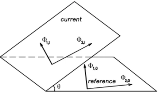
The change in a structure (e.g. damage) may be detected by monitoring the angular coherence between subspaces estimated from the reference observation set and from the observation set of a current state respectively. A state is considered as a reference state if the system operates in normal conditions (i.e. damage does not exist). Figure 1 shows a 2D example in which an active subspace (or hyper-plane) is built from two principal mode shapes.

Figure 1: Angle θ formed by active subspaces (hyper-planes) according to the reference and current states, due to a

dynamic change

4. Examples of application

4.1 Experiments in an aircraft model in different conditions

The first example consists in an aircraft model made of steel and suspended freely by means of three springs, as illustrated in Figure 2.

The fuselage is made of a straight beam of rectangular section and a length of 1.2 m. Plate-type beams connected to the fuselage form the wing (1.5 m) and tails (0.2 m). Their dimensions are detailed in Figure 3. The structure is randomly excited on the top of the left wing by an electro-dynamic shaker in the frequency range of 0-130 Hz. Eleven accelerometers are installed for capturing the dynamic responses of the structure in accordance with the set-up description given in Figure 3. Three levels of damage are simulated by removing, respectively, one, two and three connecting bolts on one side of the wing (Figure 2b). The data of this experiment was formerly used for illustrating damage detection methods based on Principal Component Analysis, Kalman model [12] and Null-subspace analysis [13]. Modal identification results were also given in [12].

a) Aircraft model b) removing of 1-3 connecting bolts

Figure 2: An aircraft model (a) and the simulated damages (b)

™ Modal identification using SOBI or BMID

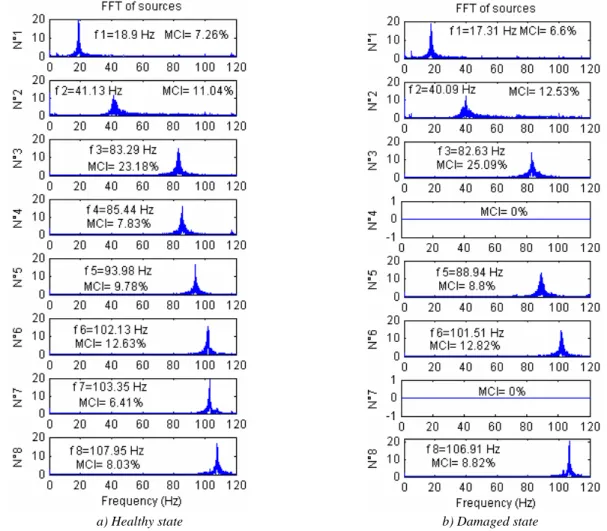
For the sake of illustrating the sensitivity of SOBI to damage occurrence, resonance frequencies and mode shapes are first identified. Figure 4a represents the first eight resonance frequencies obtained through the FFT of the identified sourcesin the healthy (undamaged) state. Some resonance frequencies are found to be relatively close, e.g. f3 (83.29 Hz) and f4 (85.44 Hz);

f6 (102.13 Hz) and f7 (103.35 Hz). These results are in perfect agreement with the identification based on the stochastic

subspace identification (SSI) method performed in reference [12].

The SOBI mode-shapes, contained in the columns of the mixing matrix A, are represented in Figure 5, where sensors n° 1-8 correspond to the wing and sensors n° 9-11 show the responses in the tails.

Let us now examine a damaged case when all the three connecting bolts are removed (Figure 2b). The FFT of the identified sources are juxtaposed to the ones corresponding to the healthy (reference) state in Figure 4b. The largest frequency variation is observed on the first frequency with 8.4% of decrease. Another very noticeable change is the disappearance of sources n° 4 and 7 when the structure is damaged. It can be also observed that the MCI of modes n° 4 and 7 in Figure 4a is quite small in comparison to the previous components - modes n° 3 and 6.Instead of 8 sources/modes, only 6 sources/modes are identified in the damaged case. The corresponding mode-shapes (dashed lines) are shown in Figure 5.

Note that the results of BMID are similar to the SOBI results and are not presented here for sake of conciseness.

™ Modal identification using Enhanced SOBI - ESOBI

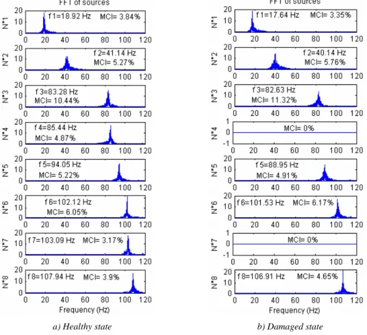
To enrich the information in the data matrix, several block rows are assembled to build the data-driven Hankel matrix defined in equation (7). In this example, the number of block rows has been fixed to 10. First, the enhancement provided by ESOBI can be noticed through the quality of the sources identified in Figure 6. The sources are now much clearer as noisy spectral components in each source are minimized with respect to Figure 4. It follows that the separation of the sources is considerably improved by the use of the data-driven Hankel matrix. ESOBI mode-shapes are also presented in Figure 7. ™ Damage detection based on the concept of subspace angle

Several tests were achieved with the aircraft model in different conditions; they are summarized in Table 1. Tests n° 1-3 correspond to healthy states but with different amplitude levels of excitation. Tests n° 4-6 correspond to damaged states with three levels of increasing damages when one, two and finally three connecting bolts are removed successively.

Table 1: Condition of tests

Test n° 1 2 3 4 5 6

Condition Exc. 1.5:0.5 Exc. 1:0.5 Exc. 1:1.5 Dam. 1 Dam. 2 Dam. 3

Since sources n° 4 and 7 are not identified in the damaged states, only six mode-shapes according to sources n° 1-3, 5, 6, 8 are considered in the subspace.

Damage detection results based on the concept of subspace angle are presented in Figure 8. To facilitate the comparison between the different methods, a common reference threshold is used, i.e. the indexes are normalized such that the maximal indexes according to the reference states (tests n° 1-3) are set to unity. The results of the proposed methods (SOBI, BMID, ESOBI and EBMID) are compared to those of Principal Component Analysis (PCA) and Null Subspace Analysis (NSA) obtained in Reference [13]. In Figure 8a, SOBI, BMID and PCA detections are displayed together. Their indexes are quite similar; however, in the PCA-based method, the first level of damage (Dam. 1) is not detected and the index corresponding to the highest level (Dam. 3) is not the biggest one. Conversely, in the SOBI and BMID-based methods, the smallest damage can be detected and the levels of damage are logically revealed. It appears in Figure 8a that the BMID-based method is the most sensitive to the presence of damage.

Detection results obtained by the use the Hankel matrix (named ESOBI, EBMID and NSA) are presented in Figure 8b. It is worth noting that when the Hankel matrix is combined with BMID, the number of block rows might be less than in ESOBI and NSA. Actually, as the measured data is first expanded using the Hilbert transform, BMID leads to double the size of the dataset. For an equivalent size of the generated data matrix, the Hankel matrix applied to BMID requires only half of the number of block rows which is used for ESOBI or NSA. Consequently the number of block rows of the Hankel matrix in EBMID should be kept moderate to accommodate the data generation. In Figure 8, the results were generated with a Hankel matrix containing 10 block rows in the case of ESOBI and NSA and 5 block rows in the case of EBMID.

a) Healthy state b) Damaged state

Figure 4: Resonance frequencies obtained by the SOBI method

a) Healthy state b) Damaged state

Figure 6: ESOBI identification of resonance frequencies by FFT of the sources

a) SOBI, BMID and PCA methods b) ESOBI, EBMID and NSA methods

Figure 8: Damage detection based on the concept of subspace angle

In conclusion, damage detection based on the concept of subspace angle using SOBI or its alternatives like ESOBI, BMID and EBMID looks very performing as illustrated in the above example. The methods are sensitive to damage even if it is small. In the modal identification step, damage occurrence may be detected, not only by looking at resonance frequency shifts but also looking at disappearance of some sources. This helps to determine the dimensionality of the problem and to construct an adequate subspace containing only compatible modes in different states of the structure.

™ Damage detection using one sensor only

The construction of the Hankel matrix before applying SOBI or BMID allows to improve identification and furthermore to detect damage even if the number of sensors is small. While SOBI cannot separate sources of narrow spectral band from only one sensor, ESOBI is able to handle this task. It is illustrated in Figure 9a when only one sensor located at point 7 (in this case, 20 block rows are used for the Hankel matrix). Similarly, identification using EBMID is presented in Figure 9b.

a) by ESOBI b) by EBMID

1 2 3 4 5 6 0 10 20 30 40 50 60 70 80 Test N° S ubs pac e a ngl e (° ) Dam 1 Dam 2 Dam 3 ESOBI EBMID

Figure 10: Damage detection by ESOBI and EBMID

Damage detection results based on the subspace angles are shown in Figure 10. ESOBI is able to detect damage levels 2 and 3 but is unable to detect damage level 1 while EBMID (using 8 block rows) is successful in distinguishing perfectly the healthy and damaged states. Thus EBMID looks more appealing when the number of sensor is small.

4.2 Damage detection in electro-mechanical devices

This industrial application concerns the case of electro-mechanical devices for which the overall quality at the end of the assembly line has to be assessed.

Figure 11: Location of the accelerometers on the electro-mechanical device: one mono-axial accelerometer on the top and

one tri-axial accelerometer on the flank of the device

A set of five good (healthy) devices and four damaged devices was considered. Dynamic responses were collected by one mono-axial accelerometer on the top and one tri-axial accelerometer on the flank of the device as illustrated in Figure 11. Only data measured in one direction on the flank (X, Y or Z in Figure 11) or on the top of the device is used for the detection. It is worth recalling that using the response measured by one sensor only, detection cannot be performed by subspace methods such SOBI and PCA. For this reason, fault diagnosis was realized in [17] using the Null subspace analysis (NSA) method based on block Hankel matrices. As it was found in [17] that fault detection is better when using the data in the Y direction, the data in this direction is exploited here to test the proposed methods.

As discussed earlier, it is also possible to construct a subspace even if only one response signal is available if BMID, SOBI are performed on the Hankel matrix. In this example, 8 block rows were used to construct the Hankel matrix. Figure 12

X Z Y Top mono-axial accelerometer Flank tri-axial accelerometer

presents the results obtained on the whole set of electro-mechanical devices. Detection results using ESOBI and EBMID are given in Figure 12a and b. It can be observed that both techniques are able to detect accurately the four faulty devices (NOk1- NOk4).

a) ESOBI based-detection b) EBMID based-detection

Figure 12: Damage detection using ESOBI and EBMID methods

(the dashed horizontal line corresponds to the maximal value for good devices)

4.3 Quality control of welded joints

The third example involves an industrial welding machine from a steel processing plan. The machine was instrumented with a mono-axial accelerometer on the forging wheel as illustrated in Figure 13. The purpose of this wheel is to flatten the welded joint.

Figure 13: Location of the accelerometer on the forging wheel of the welding machine

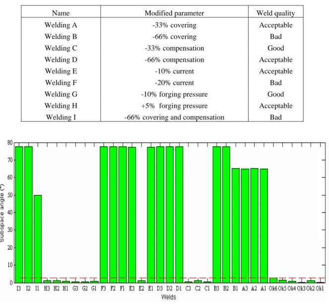
The quality of the weld depends on several parameters. Six welded joints with nominal welding parameters (Ok1-Ok6) and 27 joints with out-of-range parameters were studied. Some welding parameters were altered, namely covering, compensation, current and forging pressure as reported in Table 2. From a microscope quality control, welded joints C and G were diagnosed good, welded joints A, D, E, H were diagnosed acceptable and welded joints named B, F, I were diagnosed bad. The parameter modifications are not effectively identified by the ESOBI method. However, they can be diagnosed using the EBMID-based detection method as presented in Figure 14. In this example, the Hankel matrix is built using 10 blocks from only one response vector.

It reveals that in general, the subspace angles given in Figure 14 allow to identify the alterations reported in Table 2. For instance, the indexes of all welded joints C and G are in the same range as for healthy welded joints Ok1-Ok6 (i.e. with nominal parameters). This is in good agreement with the microscopic quality control inspections. Furthermore, the welded joints H (+5% forging pressure) and E2 (-10% current), which were diagnosed acceptable, present also small indexes. Conversely, all bad welds B, F and I are characterized by large subspace angles. Finally, it is observed that the alterations are

well identified for welds A (-33% covering); D (-66% compensation); E1 and E3 (-10% current). However, the detection indicators show that they are not proportional to the severity of the defects in the welds.

Table 2: Welds realized with altered parameters (with respect to the nominal parameters)

Name Modified parameter Weld quality

Welding A -33% covering Acceptable

Welding B -66% covering Bad

Welding C -33% compensation Good

Welding D -66% compensation Acceptable

Welding E -10% current Acceptable

Welding F -20% current Bad

Welding G -10% forging pressure Good

Welding H +5% forging pressure Acceptable Welding I -66% covering and compensation Bad

Figure 14: EBMIDdetection(the dash-dot line corresponds to the max value for healthy welded joints)

SOBI is well known as a modal identification method in the literature. It is appreciated because of its accuracy combined with its low computational cost and also because the selection of the model order is quite automatic. The accuracy of the method can be visually assessed by inspecting the modal responses (sources), for instance in the frequency domain. However, many works have shown that the main drawback of SOBI (or BMID) is the need of a number of sensors greater or equal to the number of active modes [2], [9], etc.

In this work, SOBI was applied to study the change in the dynamic behavior of mechanical systems under different conditions. The BMID technique which is an extension of SOBI has been proven to be very robust and suitable for structures with general damping. The examined examples show that the identification and detection problem using SOBI/BMID may be improved efficiently with the help of the Hankel matrices. Using ESOBI and EBMID, the detection remains still possible even if the number of available sensors is small or even reduced to one.

Acknowledgments

The authors are grateful to Jean-François Cardoso for making his extended Jacobi technique available. They would like also to thank the V2i Company for providing industrial applications.

References

[1] Kerschen G., Poncelet F., Golinval J.-C., “Physical interpretation of independent component analysis in structural dynamics”, Mechanical Systems and Signal Processing, 2007, pp. 1561-1575.

[2] Poncelet F., Kerschen G., Golinval J.-C., Verhelst D., “Output-only modal analysis using blind source separation techniques”, Mechanical Systems and Signal Processing 21, 2007, pp. 2335-2358.

[3] Zhou W., Chelidze D., “Blind source separation based vibration mode identification”, Mechanical System and Signal Processing 21, 2007, pp. 3072-3087.

[4] Farooq U., Feeny B. F., “Smooth orthogonal decomposition for modal analysis of randomly excited systems”, Journal of Sound and Vibration, 316, 2008, pp. 137-146.

[5] Popescu T.D., Manolescu M., “Blind Source Separation of Traffic-Induced Vibrations in Building Monitoring”, IEEE International Conference on Control and Automation, ICCA 2007, pp. 2101-2106.

[6] Zang C., Friswell M.I., Imregun M., “Structural damage detection using independent component analysis”, Structural Health Monitoring 3, 2004, pp. 69-83.

[7] Pontoppidan N. H., Sigurdsson S. and Larsen J., “Condition monitoring with mean field independent components analysis”, Mechanical Systems and Signal Processing 19, 2005, pp. 1337-1347.

[8] Jianping J., Guang M., “A novel method for multi-fault diagnosis of rotor system”, Mechanism and machine theory, 2009, vol. 4, n° 4, pp. 697-709.

[9] McNeil S.I., Zimmerman D.C., “Blind modal identification applied to output-only building vibration”, Proceedings of the IMAC-XXVIII, Florida, USA, February 2010.

[10] Belouchrani A., Meraim K.A., Cardoso J.F., Moulines E., “A blind source separation technique using Second - order statistics”, IEEE transactions on signal Processing 45, 1997, pp. 434-444.

[11] Overschee P. V., De Moor B., “Subspace identification for linear systems-Theory-Implementation-Applications”, Kluwer Academic Publishers, 1997.

[12] Yan A.-M., De Boe P. and Golinval J.-C., “Structural Damage Diagnosis by Kalman Model Based on Stochastic Subspace Identification”, Structural Health Monitoring, 3, 103, 2004, pp. 103-119.

[13] Yan A.-M., Golinval J.-C., “Null subspace-based damage detection of structures using vibration measurements”, Mechanical Systems and Signal Processing 20, 2006, pp. 611-626.

[14] Marchesiello S., Garibaldi L., “A time domain approach for identifying nonlinear vibrating structures by subspace methods”, Mechanical Systems and Signal Processing 22, 2008, pp. 81-101.

[15] Peeters B., De Roeck G., “Stochastic System Identification for Operational Modal Analysis: A Review”, Journal of Dynamic Systems, Measurement and Control, Transaction of the ASME, vol 123, December 2001, pp. 659-66.

[16] Golub G.H., Van Loan C.F., “Matrix computations” (3rd ed.), Baltimore, The Johns Hopkins University Press, 1996.

[17] C. Rutten, C. Loffet, J.-C. Golinval, “Damage detection of mechanical components using null subspace analysis”, 2th International Symposium ETE’2009 - Brussels, Belgium.