The electronic nose : a tool for controlling the industrial
odour emissions.
Application to the compost processing.
J. Nicolas, A.C. Romain, M. Kuske, University of Liège, Belgium
Abstract:
Different home-made electronic noses, based on commercial tin oxide gas sensors are used to identify typical sources of environmental odour nuisance. All the measurements are carried out in the field from real malodours in uncontrollable conditions, either by sampling and subsequent analysis in the lab, or by means of a mobile instrument. In spite of the influence of environmental parameters, results demonstrated the ability of such simple systems to detect and identify typical odour nuisances.
The paper analyses the type of output signal most adapted both to detect the rise of a particular odour in the background and to monitor it continuously, in order to allow a decision making in real time. Different solutions are suggested. The proposed methods are notably illustrated for a particular application : the monitoring of the odour generated by a municipal waste composting process. Results show that a technique exploiting the global response pattern of an array of gas sensors can be used to monitor continuously an atmospheric emission, in order to use the generated odour as process variable, or to predict the raise of malodour in the background, or to control an odour abatement device.
Introduction
Environmental monitoring has recently become an area of growing interest for electronic nose manufacturers [1]. Landfill sites, wastewater treatment plants, compost facilities and many industrial plants are actually located in the vicinity of towns and villages. The
malodours emanating from such activities greatly impair the comfort status requested in our civilised countries [2]. Consequently, continuous, in situ monitoring of odorous emissions is fundamental to such applications. A first goal is to predict the raise of malodour in the background before it becomes an annoyance for the surrounding [3]. A second purpose of continuous monitoring could be to use the odour as a process variable [4], aiming at a better understanding of the odour release and relating this emission to the process phase, or the problem, which caused the emission. And finally, a third and very interesting issue is the real time control of odour abatement techniques [5], such as the atomisation of neutralising agents.
Low cost and non-invasive chemical sensor arrays provide a suitable technique for in situ monitoring. Although published studies report promising results, the ability and performance of sensor arrays under realistic conditions is still discussed in the literature. Main limitations are associated with both the technology itself and its application in ever changing ambient conditions. In order to become a reality, in situ monitoring of environmental odours with electronic noses has still to overcome many difficulties, such as to take account of the influence of ambient conditions [6], to cope with the sensor drift [7], to lower the limit of detection and the limit of recognition of the sensor array [8] or to improve the reproducibility of the sensors.
During the present research, different laboratory-made electronic noses, based on
commercial tin oxide gas sensors were used to identify typical sources of odour nuisance : printing houses, paint shop in a coachbuilding, wastewater treatment plant, urban waste composting facilities, rendering plant or landfill area. All the samples were collected in the field from real malodours in uncontrollable conditions. The aim was to demonstrate the ability of such simple systems to detect and identify typical odour nuisances.
Then, portable instruments were developed to monitor in situ the odours emerging from factories or from landfills sites.
The paper analyses the type of output signal most adapted both to detect the rise of a particular odour in the background and to monitor it continuously, in order to allow a decision making in real time.
The method is illustrated on a particular application : the monitoring of the odour generated by a municipal waste composting process.
Experimental
Two methodologies are tested for the odour source identification by a sensor array. The first is based on the malodours sampling in Tedlar® bags by evacuating a pressure vessel containing the bag during about twenty minutes. Samples are taken at various distances from the source in various atmospheric and operational conditions. Some odour compounds are unstable, so all the specimen are sampled in the morning and analysed in the afternoon. Samples are analysed in the lab, by an array consisting in 12 individual commercial tin oxide gas sensors (Figaro Engineering Inc.), placed in a cubic chamber. A constant voltage is supplied continuously to the sensor heaters. The sensor resistance and the temperature and humidity of the chamber are recorded by a computer controlled acquisition board.
A complete measurement cycle consists in first drawing across the sensor chamber dry odourless air, bubbling into saturated solution (KCl in melting ice), in order to reactivate the initial semiconductor properties while keeping them at a suitable humidity, and then pumping the sampled odour across the sensor array. The useful signal is the stabilised resistance value.
For this first step, five malodours are selected from the emissions of typical activities, located near dwellings and responsible for many complaints in rural and urban environment. Two printing houses, a paint shop in a coachbuilding, a wastewater treatment plant, urban waste composting facilities and a rendering plant are investigated.
As the study aims at evaluating the ability of the array to identify each odour, the samples are collected near the source and not in the surrounding. So, in the rendering plant, samples are taken in the factory building, near the ovens in operation. The compost gases come from the sheltered compost deposit area. Sewage atmosphere is collected near the fresh sludge aerobic treatment work. The tainted air of two printing houses is sampled near the offset machine. Odorous atmosphere from the coachbuilding is collected either during or after the primer spray painting work of a car door inside the workshop.
Samples are taken at various distances from the source, for a 7-month period between March and October. For some applications, the "background" air is also considered: it is sampled far away from any odorous source.
A compost pile of the Belgium Habay city composting facility is more particularly studied. The pile of interest, located under a shelter, is constituted of household wastes with organic and inorganic material. The final pile size is about 2.5 meters high and 50 meters length. The compost aeration is achieved by turning the pile about twice a week. The composting process under the shelter lasts 8 weeks during which the compounds emission varies.
The second methodology exploits a self-made electronic nose consisting in a battery powered sensor array and a PC board, with a small keyboard and a display. Seven metal oxide sensors are placed in two 200 cm3 stainless steel boxes : four sensors from "Figaro" (TGS880, TGS822, TGS2610 and TGS842) in the first chamber and three sensors from "Capteur" (CAP01L, CAP02L, and CAP25) in the second chamber. At the beginning of the campaign, 8 sensors were used but one of them, CAP06, was quickly damaged by the harsh conditions. In both chambers, the temperature and the relative humidity are measured and recorded by the system. A small pump controlled by the computer code sucks up the ambient air through a Teflon tubing with a flow rate of 200 mL/min. Data are recorded in the local memory and downloaded in an external computer to be off-line processed by statistical and mathematical tools (Statistica and Matlab). Here, no cycling operation between pure air and tainted air is used and the considered signal is simply the raw resistance of the sensors. This detector may be moved in various spots around a given source [9].
For the compost area, some measurements of the gas emission with the mobile e-nose are performed directly on the pile in the shelter, using an emission chamber. It is a wood box roofed by Tedlar® sheet, 0.25 m height, 1.40 m long and 0.40 m wide, covering a compost area of 0.56 m². The chamber is fitted with a fan in the middle to insure the inner ventilation and with a 10 cm diameter chimney, as outlet. This chamber is placed along one side of the pile with the outlet at the top. The air velocity is measured in the middle of the outlet chimney. The estimated emission rate of the compost pile is about 15 m3/m2h. The electronic nose is connected to the chimney by a Teflon tubing. Before inflowing to the e-nose, the pumped air enters into a small dilution stainless box to avoid sensors saturation. Simultaneously, the emitted chemical compounds are adsorbed on sorbent tubes filled with a dual bed of Tenax TA/Spherocarb (Markes trademark) and further analysed in the lab by gas chromatography coupled to a mass spectrometer.
Some results further presented come also from a case study related to the odour generated by a landfill. Two kinds of odours are perceived by the neighbouring population : either the one of the fresh refuse (esters, sulphur organic compounds, solvents, …), or the one of the biogas generated by the decomposition of the organic matter under anaerobic conditions (trace elements, such as H2S, NH3 and some VOC's in a mixture essentially composed of odourless compounds : methane and carbon dioxide). Measurements are made with a mobile electronic nose.
Results and discussion
For the data processing, unsupervised multivariate methods, such as Principal Component Analysis (PCA), are able to highlight some clusters that fit the odour sources without making any prior assumption about the membership of an observation to a given class. It proves the performance of the system and eventually stresses a problem which is responsible of the largest part of the variance in the data, such as the sensor drift [7]. Nevertheless, in order to calibrate a model which can be embedded in a field odour annoyance detector designed for real-time odour identification, a supervised pattern recognition technique, such as the discriminant function analysis (DFA), must be applied. By indicating to the method that the target grouping feature for the classification is the origin of the odorous emission, the system is able to recognise rather well the different investigated sources.
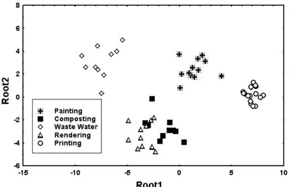
Figure 1 shows the scatter plot of 59 observations performed around the 5 sources above mentioned in the plane of the two first discriminant functions (roots) of a DFA.
Fig. 1: : Results of a Discriminant Function Analysis in the plane of the two first roots for 59 samples from 5 odorous sources in the environment.
Differences between samples can clearly be observed: "solvent type" odour on the right part of the diagram and "waste type" odour on the left side. The vertical axis separates the "humid odour" of the waste water from the group "compost" and "rendering". The similarity of some chemical compounds (especially ammonia, aldehydes, alcohols and fatty acids), identified in those two last odours, can explain the similarity of the two corresponding patterns.
That means that as long as the data set intrinsically contains the information about a given property, like the odour type, a supervised method is able to classify the data according to that property. When the data processing method is unable to classify the observations according to the odorous tonality, that could be due to a wrong initial selection of the sensors in the array. Sensors obviously react to many chemicals whether they smell or not and the right sensor selection is primordial when the recognition of the odorous tonality of the gas emission is the target of the study.
As the major purpose of the present approach is to predict which group new samples belong, it is necessary to validate the model with "unknown" samples, i.e. observations which were not in the data set used for the model calibration. We showed that such validation for 10 new cases gives a correct classification [2].
Of course, such discrimination between 5 different odorous sources doesn't present much practical interest. This academic case study just shows that, in spite of environmental constraints, the identification of real malodours is feasible with a simple sensor array and suitable data processing methods. The explanation of the role of the sensors in the
classification confirms that the recognition is not fortuitous. Further more practical studies in landfill areas show however that a recognition model can be calibrated in the same manner to distinguish the fresh refuse odour from the landfill gas one. Such result is particularly useful for the landfill manager: detecting the raise of the landfill gas odour in the background of the fresh waste odour could indicate a problem, like a leak in the landfill gas collection network.
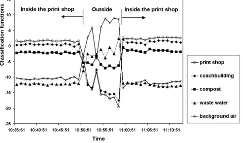
When using DFA, the classification into the different groups is achieved thanks to the classification functions, which are provided by the procedure as standard results, besides discriminant functions, and which constitute the discrimination model itself. The DFA procedure generates automatically as much classification functions than there are different groups (for example, 5 if there are 5 odour sources). Such simple model leads to the fast classification of a new observation in a known group. So, those classification functions can also be used as "odour signal". Though they show very bad correlation with the intensity measured in the field, their selectivity to a given odour can be exploited for the continuous odour monitoring. Figure 2 shows such result obtained for 5 sources (print shop,
coachbuilding, compost, waste water and background air, far from any odorous source) and with a mobile detector. Five classification functions are computed by the DFA method, during the learning phase (model calibration step). They are linear combinations of the 8 sensor signals used in the present case. An observation is classified into the group for which it has the highest classification score. During the validation phase, the same mobile detector is moved to various spots around a given source and, at each sampling time of the data logger, the data from the sensor signals are inserted into each previously calibrated classification function to develop a classification score for each group. Figure 2 shows the graphical
evolution of the five calibrated classification functions when the detector is moved around the print shop. The scaling of the horizontal time axis is unessential: it shows only that the mobile detector is continuously moving away from the source. The function corresponding to the print shop has, effectively, the highest value when the detector is in the printing shop, but it suddenly drops when the detector is moved outside the shop, and increases again when the technician moves back inside. As expected, the classification function characterising the outside atmosphere is the "background" one.
Figure 2 : Evolution of the DA classification functions, resulting from the learning phase with five sources, when the mobile detector is moved around in the print shop.
Such classification functions could be used as global "odour signal": that shows the interest of working with an array of sensors rather than with individual sensors. Using one of the sensor elements, preferably that with the highest sensitivity towards the identified
substances, should be a rather easy solution, but such single sensor is sensitive to every sources, so, its signal cannot be used to detect the rise of a particular odour among other ones. In this case, the procedure should thus always include two steps : a first identification of the odour by a classification technique, followed by the monitoring of the intensity of the global odour.
To avoid the first step of the procedure, a better solution is thus to consider as "odour signal" a mathematical combination of all the sensor signals. However, the above described DFA approach calibrates the classification functions only on the basis of a qualitative recognition of the source. The purpose of DFA is only to build a model which allocates an observation to a given group: the membership of the group is notified as "yes" or "no". So, the value of the classification function doesn't represent any "level of membership" to the given group. A way to build a quantitative odour signal from the sensor responses is to calibrate a model by regression with a quantitative variable, representing an "intensity level".
This approach is illustrated for the landfill case study. The operator performs measurements at some different locations on the landfill area : either in the vicinity of fresh waste,
sometimes when the trucks pour out the refuse, sometimes when the waste is at rest, or at various distances from a landfill gas extraction well. At each location, he also notes his feeling of odour intensity on a 4 level scale. A total of 141 observations are carried out with that procedure : 69 around "fresh waste" (including 21 observations with intensity 0), and 72 around "biogas" (including 24 zero-intensity observations). Then, different regression
techniques are applied to build a model fitting the measured intensity and which should be able to predict the intensity of the generated odour. Multilinear Regression (MLR) on the original measured sensor signals (resistances) provides a rather good model, which predicts an intensity value in agreement with the measured one in 67 % of the cases. The resulting model, however, is a pure mathematical construction, which is convenient to predict intensity values inside the training sample, but which is less adapted to the prediction of new data [11].
Using the results of an unsupervised classification method, such as the factors supplied by a Principal Component Analysis (PCA), has a good chance to produce a more physical model, making more "sense" from a physical standpoint [12]. Indeed, the principal component regression (PCR) includes in the model the first principal component, which is already well correlated with the odour intensity, and the second one, which separates "biogas" from "fresh waste". Including the third one in the regression provides a model which predicts the
measured intensity in 69 % of the cases. Of course, the model converges towards the MLR one when the 3 remaining principal components are added. As this model MLR is worse than the model based on 3 principal components, it seems that some of the initial variables were not relevant for the prediction of the odour intensity.
Finally, Partial Least Squares regression (PLS), which captures the greatest amount of variance, like PCA, and also achieve correlation with the predictor variable (here the
intensity), like MLR, will probably provide the most adapted model for the intensity prediction. Indeed, testing PLS regression on the 141 observations on the landfill shows that the model provides 71 % of intensity prevision in agreement with the measured one. Moreover, like PCA, the PLS provides the classification of observations in two groups. Consequently, it should be used as sole tool, both to identify the source of the odour and to predicting its intensity [10]. Figure 3 shows the 3D scatterplot of the observations. Vertical axis is the predicted intensity level and the two horizontal ones are the two first "latent variables" (the equivalent of principal components in PCA) extracted by the procedure. As shown, the "fresh refuse" observations are quite well separated from the "biogas" ones.
Figure 3 : Predicted odour intensity around a landfill site from a PLS model
This former example used the operator's intensity feeling as dependant variable of the regression. Other dependant variables may obviously be used, depending on the feature which must be highlighted.
Another regression example is illustrated in the case of the gas emission of the compost pile. The objective of this application is to verify that the gas emission of a pile is an index of the composting process. The relations between the e-nose measurement, the chemical analysis and the process information are investigated, during a 11 days period. About two hundreds compounds are identified in each sample. They are grouped in 15 chemical families.
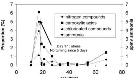
When examining the evolution of the chemical composition with the age of the compost pile, it is noted that some chemical families appears in the middle of the composting process, some others at the beginning of the self heating phase and others at the end of the maturation phase. So, a single sensor signal can't represent an adequate indicator of the whole process evolution. Some sensor responses decrease at the end of the composting process while other signals grow at the same time. The advantage of using an array of sensor and a global "odour signal" is illustrated to highlight two kinds of events. The first one is a "stress" event. As seen on figure 4, peaks of nitrogen compounds, carboxylic acids, ammonia and chlorinated compounds appear on day 17. They are characteristic of a stress episode caused by the absence of aeration : there was no turning of the pile for 5 days.
Figure 4 : Evolution with compost age of relative proportion of 4 chemical families, showing a "stress" event.
A first specific indicator is thus constructed by relating the sensor signals to the four families of compounds emitted during that "stress" phase. It is constructed by a canonical correlation analysis. Such analysis aims at studying the relationship between two sets of variables, each of which being able to contain several variables. The purpose of that procedure is to
summarize or explain the relationship between the two sets of variables by finding a small number of linear combinations from each set that have the highest correlation possible between the sets. The first combinations of each set are generally selected, as their
correlation coefficient is the higher. The main difference with standard multilinear regression is that canonical correlation analysis allows several "dependant" variables, and not only one. Figure 5 shows the time evolution of that first combination of the sensor signals applied to the whole data set obtained by the continuous signal monitoring for 11 days.
Figure 5 : Time evolution of the first root of a canonical correlation analysis calibrated with ammonia, nitrogen compounds, carboxylic acids and chlorinated compounds.
The root value remains around zero unless during the 17th day when it goes beyond 2 : that is precisely a "stress" day, as the compost windrow was not turned for 5 days.
A second event is the end of the thermophilic phase (start of compost maturation)
characterized by the release of abiogenic substances, i.e. substances generated by pure chemical reactions and which are not issued of the micro-organisms degradation. We
particularly observed the release of furans and ketones With the same set of observations, a second indicator is thus constructed by relating the sensor signals, this time to those
compounds emitted during the "final" phase : furans and ketones. Figure 6 shows the time evolution of that root for the whole data set. The root value rises for day 68, when the compost reaches the end of its composting phase.
Figure 6 : Time evolution of the first root of a canonical correlation analysis calibrated with furans and ketones.
Thus, with the same sensor signals, different types of indicators can be constructed,
depending on the type of event they intend to highlight. The calibration of such indicators just needs the results of a systematic GC-MS analysis, which is a one-shot operation. Once calibrated, the indicators could be used for on-line monitoring of the compost process. Conclusion
The paper shown the ability of the e-nose to monitor various kinds of odorous (and not odorous) events simultaneously. Indeed with the development of specific models, it is
possible to monitor at the same time different process parameters with the same instrument. That proves the interest of working with an array of gas sensors and with a global signal pattern rather than with the individual responses of sensors. The various applications
demonstrate that, despite many remaining problems inherent in chemical sensors, electronic nose present a lot of advantages to monitor gas emission with respect to classical spotted measurements.
References
[1] Bourgeois, W., Romain, A.-C., Nicolas, J., Stuetz, R. M.: The use of sensor arrays for environmental monitoring: interests and limitations. J. Environ. Monit. 5 (2003) pp. 852-860.
[2] Romain, A.-C., Nicolas, J., Wiertz, V., Maternova, J., Andre, P.: Use of a simple tin oxide sensor array to identify five malodours collected in the field. Sensors actuators B 62 (2000) pp. 73-79.
[3] Di Francesco, F., Lazzerini, B., Marcelloni, F., Pioggia, G.: An electronic nose for odour annoyance assessment. Atmospheric environment 35 (2001) pp. 1225-1234
[4] Bachinger, T., Haugen, J. E.: Process Monitoring, in Handbook of Machine Olfaction (Ed.: J. W. Gardner). Weinheim: Wiley-VCH 2002.
[5] Gostelow, P., Parsons, S. A., Stuetz, R. M.: Odour measurements for sewage treatment works. Water Research 35 (2001) pp. 579-597.
[6] Romain, A.-C., Nicolas, J., André, Ph.: In situ measurement of olfactive pollution with inorganic semiconductors - Limitations due to humidity and temperature influence. Seminars in Food Analysis 2 (1997) pp. 283-296
[7] Romain, A.C., André, Ph, Nicolas, J.: Three years experiment with the same tin oxide sensor arrays for the identification of malodorous sources in the environment. Sensors and actuators B 84 (2002) pp. 271-277
[8] Nicolas, J., Romain, A.C.: Establishing the limit of detection and the resolution limits of odorous sources in the environment for an array of metal oxide gas sensors. Sensors and Actuators B 99 (2004) pp. 384-392
[9] Nicolas, J., Romain, A-C., Wiertz, V., Maternova, J., André, Ph.: First trends towards a field odour detector for environmental applications. Proceedings ISOEN 99, Tübingen, September, 20-22, 1999 – pp. 368-371
[10] Nicolas, J., Romain, A.C., Maternova, J.: Chemometrics methods for the identification and monitoring of an odour in the environment with an electronic nose, in Sensors and Chemometrics (Ed. M.T. Ramirez). Kerala: Research Signpost 2001, pp. 75-90.
[11] Nicolas, J., Romain, A.C., Monticelli, D., , Maternova, J., André, Ph.: Choice of a suitable E-nose output variable for the continuous monitoring of an odour in the environment. Proceedings of ISOEN2000, Brighton, July, 20-24, 2000 – ed. By J.W. Gardner and K.C. Persaud - pp. 141-146
[12] Wise, B.M., Gallagher, N.B.: PLS_Toolbox 2.0 for use with MATLABTM. Manson: Eigen Research, Inc. 1998 - pp.320.