HAL Id: hal-01150814
https://hal.archives-ouvertes.fr/hal-01150814
Submitted on 11 May 2015HAL is a multi-disciplinary open access archive for the deposit and dissemination of sci-entific research documents, whether they are pub-lished or not. The documents may come from teaching and research institutions in France or abroad, or from public or private research centers.
L’archive ouverte pluridisciplinaire HAL, est destinée au dépôt et à la diffusion de documents scientifiques de niveau recherche, publiés ou non, émanant des établissements d’enseignement et de recherche français ou étrangers, des laboratoires publics ou privés.
A Simple Method to Calibrate Kinematical Invariants:
Application to Overhead Throwing
Antoine Muller, Coralie Germain, Charles Pontonnier, Georges Dumont
To cite this version:
Antoine Muller, Coralie Germain, Charles Pontonnier, Georges Dumont. A Simple Method to Cali-brate Kinematical Invariants: Application to Overhead Throwing. 33rd International Conference on Biomechanics in Sports (ISBS 2015), Jun 2015, Poitiers, France. �hal-01150814�
A SIMPLE METHOD TO CALIBRATE KINEMATICAL INVARIANTS:
APPLICATION TO OVERHEAD THROWING
Antoine Muller
1,2, Coralie Germain
1,2, Charles Pontonnier
1,2,3and Georges
Dumont
1,2Ecole Normale Supérieure de Rennes, Bruz, France
1IRISA/INRIA Rennes, Rennes, France
2Ecoles Militaires de Saint-Cyr Coëtquidan, Guer, France
3The aim of this paper is to present a simple calibration method aimed at optimizing the kinematical invariants of a whole body motion capture model, meaning limb lengths and some of the marker placements. A case study and preliminary results are presented and give encouraging insights about the generalized use of such a method in motion analysis in sports.
KEY WORDS: Subject-specific model, Inverse kinematics, Optimization, Baseball,
INTRODUCTION: Matching lengths and joint centers of a generic biomechanical model with the dimensions of a specific subject is of importance in motion analysis, especially in sports biomechanics. A subject-specific calibrated model has more chances to catch the specificities of a given motion than a generic of badly scaled model. Andersen et al. (Andersen, 2010) proposed a well fashioned method to calibrate kinematical invariant properties of biomechanical models thanks to motion capture. It consists in finding the set of joint angles and kinematical invariants (e.g. limb lengths, or marker placements) minimizing the error between real and reconstructed markers on the whole capture under constraints maintaining joints consistency. The aim of the current paper is to propose a simple two-stage method to calibrate kinematical invariants, aimed at being used as the first step of an inverse dynamics motion analysis pipeline. An application to overhead throwing is proposed and results are discussed.
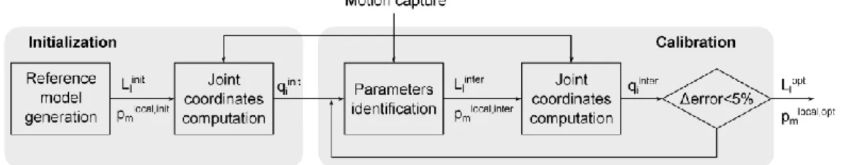
METHODS: The calibration method used in this study is structured in 2 steps (Figure 1). The first step initializes the limb lengths, the marker placements and the set of joint angles. In the second step, the calibration itself is performed. The kinematical invariants are optimized. These calibrated parameters can be used to study the kinematical features (e.g. joint angles, joint velocities…) of the current motion or of any motion realized by the same subject.
Figure 1: Calibration pipeline
Initialization: The whole body skeletal model used in this study is composed of 21 rigid segments linked by 17 joints and exhibits 32 degrees of freedom. The lower limb model is based on Klein Horsman’s model (2007). The de Zee’s spine model (2007) is integrated to the trunk model. The upper limb model is based on Holzbaur’s model (2005). A uniform scaling in all directions (Rasmussen, 2005) is used to initialize kinematical invariants parameters on the basis of the current subject’s size.
The initialization of the joint angles is an inverse kinematics step. This step aims at computing a set of joint coordinates 𝒒𝑖 = 𝒒(𝑡𝑖) from a motion capture, for 𝑖 = 1, 2, … , 𝑁.
Where 𝑁 is the number of frames and 𝒒𝑖 is a 𝑛𝑞-column vector, where 𝑛𝑞 is the number of joint coordinates. The inverse kinematics step can be solved with 𝑁 optimization problems:
Find 𝒒𝑖
(1) which minimize 𝐹(𝒒𝑖, 𝒑𝑚𝑙𝑜𝑐𝑎𝑙, 𝒍) = ∑‖𝒑𝑚𝑔𝑙𝑜𝑏𝑎𝑙(𝒒𝑖) − 𝒑𝑚,𝑟𝑒𝑎𝑙(𝑡𝑖)‖
𝑚
2
where 𝒑𝑚,𝑟𝑒𝑎𝑙(𝑡𝑖) is the position of the 𝑚-th real marker at the time 𝑡𝑖, obtained by the motion capture. 𝒑𝑚𝑔𝑙𝑜𝑏𝑎𝑙(𝑞𝑖) is the global position of the 𝑚-th reconstructed marker at frame 𝑖. At this stage, the local coordinates of the markers 𝒑𝑚𝑙𝑜𝑐𝑎𝑙 – the coordinates relative to the segment coordinates system – are fixed and 𝒑𝑚𝑔𝑙𝑜𝑏𝑎𝑙(𝑞𝑖) are reconstructed thanks to homogeneous transforms.
Calibration: The aim of this calibration is to identify the optimal kinematical invariants for each subject. The optimized kinematical invariants are some of the limb lengths 𝒍̂ and some of the marker placements 𝒑̂𝑚𝑙𝑜𝑐𝑎𝑙.The method used in this study is inspired by the methods developed by Andersen et al. (2010) and Reinbolt et al. (2005). The set of joint coordinates obtained from the initialization step is defined as 𝒒𝑖𝑖𝑛𝑖𝑡. The calibration consists in an optimization loop, divided into two stages (Figure 1). The first stage aims at finding the optimal parameters (𝒍̂, 𝒑̂𝑚𝑙𝑜𝑐𝑎𝑙). Equation (2) describes the optimization problem applied on a set of frames 𝑁𝑐, where 𝑁𝑐 could be a sub-set of 𝑁 randomly generated by bootstrapping, to reduce the computation time.
Find 𝒑𝒂𝒓𝒂𝒎 = [𝒍̂, 𝒑̂𝑚𝑙𝑜𝑐𝑎𝑙]𝑇 (2) which minimize 𝐺(𝒑𝒂𝒓𝒂𝒎, 𝒒𝑖𝑖𝑛𝑡𝑒𝑟) = ∑ ∑‖𝒑𝑚𝑔𝑙𝑜𝑏𝑎𝑙(𝒑𝒂𝒓𝒂𝒎, 𝒒𝑖𝑖𝑛𝑡𝑒𝑟) − 𝒑𝑚,𝑟𝑒𝑎𝑙(𝑡𝑖)‖ 𝑚 𝑖 2
where 𝒒𝑖𝑖𝑛𝑡𝑒𝑟 represents the joint coordinates computed in the last inverse kinematics step (e.g. for the first loop, 𝒒𝑖𝑖𝑛𝑡𝑒𝑟 = 𝒒𝑖𝑖𝑛𝑖𝑡).
The second stage of the calibration step (Figure 1) aims at actualizing the joint coordinates with the updated (𝒍̂, 𝒑̂𝑚𝑙𝑜𝑐𝑎𝑙). This inverse kinematics step is solved as shown in equation (1). For each iteration, a reconstruction error is computed. This error corresponds to the average distance between a reconstructed marker and the associated real marker. The optimization loop stops when the variation of the mean error between two iterations is below 5%.
Case study: The aim of this case study was to validate the method presented above. For this purpose, this method has been implemented in Matlab® and a visualization tool has been designed thanks to the Simmechanics toolbox. The results of the calibration and the inverse kinematics were compared to the ones obtained with the Andersen at al. (2010) method that is already implemented in the AnybodyTM modeling software (Anybody Technology). This software is widely used in the biomechanics community. A classical motion capture analysis was used.
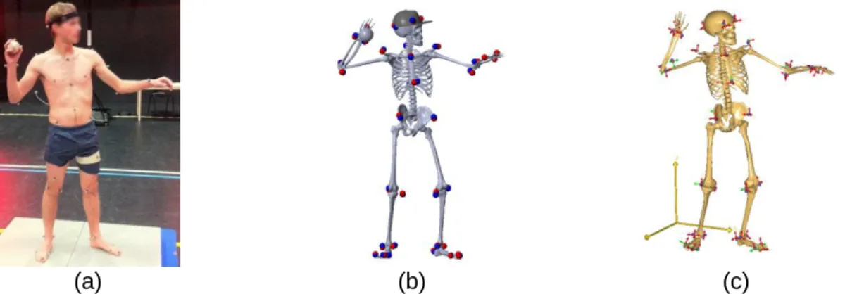
One pilot trial was performed on a single subject in our lab. The subject – a 60 kg, 170 centimeters, 24 years old man – was not specially trained to baseball throwing. This experiment was composed of 4 overhead throwing. Each of these took about 3 seconds. 40 motion capture markers were placed (Figure 2(a)) on the whole body. The markers were recorded at 100 Hz using a Vicon motion capture system. The addition of asymmetric markers helped to the reconstruction of marker trajectories. Then, these markers trajectories were filtered using a 4-th order Butterworth low pass filter with a cut-off frequency of 5 Hz and no phase shift.
For each trial, both calibration methods were applied. Each limb length was optimized. Additionally, placements of the markers for uncertain bony landmarks were optimized. Then, optimized limb lengths and markers placements of a given trial were used to perform inverse kinematics on all the trials to test the inter-trial robustness of the method.
(a) (b) (c)
Figure 2: Full body model and marker placements during the throwing the pilot trial. (a) – Experimental setup for Motion capture; (b) – Our model; (c) – AnyBodyTM
model.
RESULTS AND DISCUSSION: Table 1 summarizes the limb lengths 𝒍̂∗ obtained with our
calibration (Figure 2(b)) and the ones obtained in AnyBodyTM (Figure 2(c)) for all trials. The lengths of the distal members were not compared due to their dependency to the associated markers location. Markers placement comparison seemed difficult to achieve since their local coordinates were not expressed in the same way for both models.
Table 1: Comparison of the limbs lengths calibration methods using different motion capture.
𝝈𝒏 : normalized standard deviation. 𝜺𝒏 : mean of the relative difference between methods.
AnybodyTM calibration Our calibration 𝒍̂∗ [cm] Throw 1 Throw 2 Throw 3 Throw 4 𝜎𝑛 [%] Throw 1 Throw 2 Throw 3 Throw 4 𝜎𝑛 [%] 𝜀𝑛 [%] Pelvis width 15.55 15.55 15.55 15.55 0.02 14.26 14.37 14.21 14.27 0.32 8.19 Thigh lengths 41.48 41.64 41.47 41.69 0.23 42.49 42.56 42.36 42.49 0.14 2.18 Shank lengths 39.61 39.44 39.48 39.49 0.13 39.67 39.61 39.61 39.73 0.11 0.38 Trunk height 55.33 55.67 54.78 54.81 0.64 53.11 53.11 52.94 53.04 0.11 3.80 Upper arm lengths 28.74 28.48 28.38 27.91 0.83 29.81 29.93 30.03 30.04 0.28 5.56 Lower arm lengths 27.52 27.47 27.36 27.85 0.54 26.04 25.97 25.84 25.89 0.27 5.87
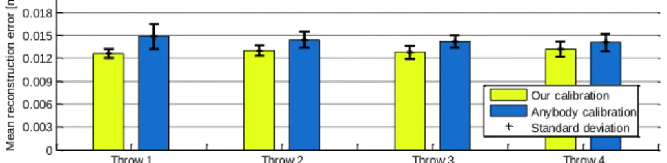
For both methods, the optimized limbs lengths were relatively unaffected by the motion capture used as input. Moreover, even if both methods gave slightly different results, they also gave consistent lengths in accordance with the literature. It is therefore interesting to extend this study to different types of motion to test its robustness. Figure 3 compares the mean marker error obtained for each trial after calibration with both methods. Trials were here self-calibrated, meaning that the calibration was realized with the studied trial. The order of magnitude of the error was the same for both methods and was arguably reproducible from one capture to one other. Moreover, the standard deviation seemed to be low compared to the error, meaning that the error remained relatively constant against time. This observation tends to show that the remaining reconstruction error was due to non-calibrated invariants. The results presented above are encouraging since the calibration method showed comparable results to the one of AnyBodyTM. However, the small sample size of trials ask for further comparisons to be completely valid.
Table 2 shows the reconstruction error for each trial from different calibrations using our calibration method. The standard deviation of these errors was valued at 0.4 mm. Thus, after the inverse kinematics step, the reconstruction error was relatively unaffected by the trial used to calibrate. Furthermore, the use of only one calibration for a set of motion capture seems to be sufficient.
Figure 3: Mean distance between a reconstructed marker and the associated real marker and standard deviation over four throwing motion capture with the two methods
For a given throwing trial, the smallest error was expected when the calibration was realized with this trial (diagonal elements). This result was apparent in the first three motion capture contrary to the fourth. The difference observed was very low in comparison with the error. It was probably due to the fact that, in the parameters identification step, only a sub-set of all the motion capture frames was used. For the study, this sub-set was chosen randomly. It is therefore interesting to deepen this work in defining a paradigm enabling a consistent choice for this sub-set.
Table 2: Mean markers error depending on the trial used for calibration
Mean reconstruction error [m]
Calibration
Throw 1 Throw 2 Throw 3 Throw 4
Mo ti on c ap ture Throw 1 0.0126 0.0141 0.0138 0.0142 Throw 2 0.0132 0.0130 0.0130 0.0132 Throw 3 0.0131 0.0131 0.0128 0.0132 Throw 4 0.0133 0.0132 0.0131 0.0132
CONCLUSION: The current paper aimed at presenting a simple calibration method for kinematics invariants based on a two-stage optimization scheme. Results obtained on overhead throwing motions showed encouraging results, comparable to the state of the art in terms of accuracy and repeatability. Further investigations are warranted to test the robustness of the method and to add other kinematical invariants (e.g. rotation axes). This work is a first step and further developments to include whole-body inverse dynamics and muscle forces estimation are currently ongoing. This work aims to develop a simple tool ready to use for motion analysis, in particular for sports applications such as training, motion optimization or injury prevention.
REFERENCES:
Andersen, M.S., Damsgaard, M., MacWilliams, B. & Rasmussen, J. (2010). A computationally efficient optimisation-based method for parameter identification of kinematically determinate and over-determinate biomechanical systems. CMBBE, 13(2), 171-183.
De Zee, M., Hansen, L., Wong, C., Rasmussen, J. & Simonsen, E.B. (2007). A generic detailed rigid-body lumbar spine model. Journal of biomechanics, 40(6), 1219-1227.
Holzbaur, K.R., Murray, W.M. & Delp, S.L. (2005). A Model of the Upper Extremity for Simulating Musculoskeletal Surgery and Analyzing Neuromuscular Control. Annals of Biomedical Engineering, 33(6), 829-840.
Horsman, M.K., Koopman, H.F.J.M., Van der Helm, F.C.T., Prosé, L.P. & Veeger, H.E.J. (2007). Morphological muscle and joint parameters for musculoskeletal modelling of the lower extremity.
Clinical biomechanics, 22(2), 239-247.
Rasmussen, J., Zee, M.D., Damsgaard, M., Christensen, S.T., Marek, C. & Siebertz, K. (2005). A general method for scaling musculo-skeletal models. Int. Symp. on computer simulation in
biomechanics.
Reinbolt, J.A., Schutte, J.F., Fregly, B.J., Koh, B.I., Haftka, R.T., George, A.D., & Mitchell, K.H. (2005). Determination of patient-specific multi-joint kinematic models through two-level optimization. Journal of biomechanics, 38(3), 621-626.
Throw 1 Throw 2 Throw 3 Throw 4
0 0.003 0.006 0.009 0.012 0.015 0.018 M e a n r e co n st ru ct io n e rr o r [m ] Our calibration Anybody calibration Standard deviation