HAL Id: hal-01186444
https://hal.archives-ouvertes.fr/hal-01186444
Submitted on 28 Aug 2015
HAL is a multi-disciplinary open access
archive for the deposit and dissemination of
sci-entific research documents, whether they are
pub-lished or not. The documents may come from
teaching and research institutions in France or
abroad, or from public or private research centers.
L’archive ouverte pluridisciplinaire HAL, est
destinée au dépôt et à la diffusion de documents
scientifiques de niveau recherche, publiés ou non,
émanant des établissements d’enseignement et de
recherche français ou étrangers, des laboratoires
publics ou privés.
Learning to Hash Faces Using Large Feature Vectors
Cassio dos Santos Jr., Ewa Kijak, Guillaume Gravier, William Robson
Schwartz
To cite this version:
Cassio dos Santos Jr., Ewa Kijak, Guillaume Gravier, William Robson Schwartz. Learning to Hash
Faces Using Large Feature Vectors. International Workshop on Content-based Multimedia Indexing,
2015, Prague, Czech Republic. �hal-01186444�
Learning to Hash Faces Using Large Feature Vectors
Cassio E. dos Santos Jr.
∗, Ewa Kijak
†, Guillaume Gravier
†, William Robson Schwartz
∗∗ Department of Computer Science, Universidade Federal de Minas Gerais, Belo Horizonte, Brazil
† IRISA & Inria Rennes (CNRS, Univ. Rennes 1), Campus de Beaulieu, Rennes, France
[email protected], [email protected], [email protected], [email protected] Abstract—Face recognition has been largely studied in past
years. However, most of the related work focus on increasing accuracy and/or speed to test a single pair probe-subject. In this work, we present a novel method inspired by the success of locality sensing hashing (LSH) applied to large general purpose datasets and by the robustness provided by partial least squares (PLS) analysis when applied to large sets of feature vectors for face recognition. The result is a robust hashing method compatible with feature combination for fast computation of a short list of candidates in a large gallery of subjects. We provide theoretical support and practical principles for the proposed method that may be reused in further development of hash functions applied to face galleries. The proposed method is evaluated on the FERET and FRGCv1 datasets and compared to other methods in the literature. Experimental results show that the proposed approach is able to speedup 16 times compared to scanning all subjects in the face gallery.
I. INTRODUCTION
Face recognition consists of three tasks described as fol-low [1]. Verification considers 1-1 tests where the goal is to verify whether two samples belong to the same subject.
Identificationconsists in a 1-N test where a sample is compared
to a gallery containing N subjects. Open-set is the same as identification but considers that the probe subject may not be enrolled in the gallery. In this work, we consider face identification, which is important for numerous applications, including identification of clients in social media, human-computer interaction, search for interviews of a specific person in TV broadcast footages, search for suspects in videos from cameras for forensics or surveillance purposes, and in image databases. These applications present distinct aspects and challenges that have been investigated on other works and, as a result, it is possible to find a large variety of face identification approaches in the literature.
Although several works for face identification have been developed, only few of them target scalability regarding large galleries [2]–[4]. Our goal is to develop an approach to return the correct identity of a probe sample in an affordable time even for galleries containing thousands of subjects. One possible approach is to reduce the computational burden to test pairs of probe and subject in the gallery. However, the number of tests required to return the correct identity will be linear to the number of enrolled subjects. We are interested in, given a probe, discard with low computational cost most of the candidates in the gallery that are less likely to correspond to the identity of the probe sample. In this paper, we achieve both low cost to filter candidates and sub-linear complexity with respect to the number of subjects.
To address face identification on large galleries, we con-sider the well-known LSH method for large general purpose
datasets and PLS applied to face identification using feature combination. The proposed approach consists in generating hash functions based on PLS and large feature vectors to create a short list of candidates for further use in face identification methods. Theoretical and practical discussion presented on the
design of the algorithm imply that at least dlog2(N )e hash
function evaluations are required to compute the candidate list for a gallery with N subjects. Furthermore, the combi-nation of different feature descriptors using PLS is shown to increase significantly the recognition rate with the candidate list compared to single feature descriptors. Provided that hash functions are based on PLS, a simple dot product is required to compute each hash function, thus, reducing the time necessary to retrieve the candidate list.
The remainder of the paper is organized as follow. In Section II, we review works in the literature related to face identification and large-scale image retrieval. In Section III, we present the hashing scheme based on PLS regression. In Section IV, we evaluate the proposed approach on the FRGC and FERET datasets. Finally, we conclude this paper with final remarks in Section V.
II. RELATEDWORKS
Due to lack of space, we briefly review face identification methods based on regular 2D images We refer the reader to [5] for a more detailed presentation of different methods for face identification.
A. Face Identification
Face identification methods are divided in two cate-gories [6]: appearance-based (holistic), feature-based (local). In holistic methods [3], [7], the whole face image is repre-sented using feature descriptors extracted from a regular grid or from overlapping rectangular cells. The advantage of holistic methods is the easy encoding of overall geometric disposition of patches in the final descriptor. However, a preprocessing step is usually required to account for misalignment, lightning conditions, and pose variations. Feature descriptors commonly employed in holistic methods include local binary patterns (LBP) and Gabor filters [7].
Methods based on local description [8], [9] represent face images in a sparse manner by extracting feature descriptors from regions around fiducial points, such as nose tip or corners, eye and mouth. Regarding the detection of interest points, the authors in [9] consider a fiducial point detector while the au-thors in [8] estimate salient points in the face image for further match with other salient points from other face images. The advantage of local description is the robustness regarding pose changes and partial occlusions. That is, even if some points are
occluded or shaded, other points can be used for identification, differently from the holistic representation. Although robust, local description methods neglect overall appearance of the face image and they often produce ambiguous description since only a few pixels of the image are considered to compute the final descriptor.
In recent years, sparse representation-based classification (SRC) [10] has been exploited, yielding good performances in face identification datasets. The method consider probe images as a linear combination of a dictionary composed by samples in the face gallery. Although the original approach requires a large number of samples per subject, SRC has been further extended to support single samples [11]. In [12], the authors propose to represent the dictionary as centroids of subject samples and their relative differences in order to account for uncontrolled acquired images in the face gallery.
B. Large-scale Image Retrieval
In the last section, we discussed works related to face identification and, since we are interested on methods to speedup face identification in large face galleries, in this section, we discuss some works related to large-scale image retrieval and scalable face identification. The goal in image retrieval is to retrieve the closest image in the gallery to a test sample considering a similarity metric between two or more images. In face identification, the metric is related to the likelihood that an image, or a set of images, represents the same subject in the face gallery. Although efficient algorithms to the exact closest match exist, they result in poor performance on high dimensional feature spaces, which is often the case when dealing with image retrieval. To solve this problem, several algorithms for approximate search have been proposed in the literature, including the popular locality sensing hashing (LSH) [13] which we further describe.
The idea of LSH is to use hash functions to map similar inputs to the same position in a hash table. Regarding the type of the hash function considered, LSH methods can be divided in two categories [13]: data independent and data dependent. On one hand, data independent hash functions are defined regardless of the data distribution and their main advantage is the fast enrollment of new samples in the dataset. An example of data independent hash function is presented in [2] and consists in generating random regression vectors using a p-stable distribution. On the other hand, data dependent hash functions analyze the data to take more advantage of the data distribution. A hash function based on maximum margin separation among images in the gallery was presented in [14]. Regarding fast face identification, methods based on dis-tance metrics usually employ compact representation of face images, such as binary patterns [15] to speedup image-image comparisons. In SRC methods, fast optimization algorithms have been proposed to compute the linear transformation among probe and gallery samples [16]. Although the afore-mentioned methods provide considerable speedup over probe-gallery pair comparison, their complexity depends on the number of subjects enrolled in the face gallery. To tackle this problem, a rejection tree was proposed in [3] to narrow down quickly the number of subjects in the gallery to a small list of candidates, and a rejection cascade was proposed in [4] to
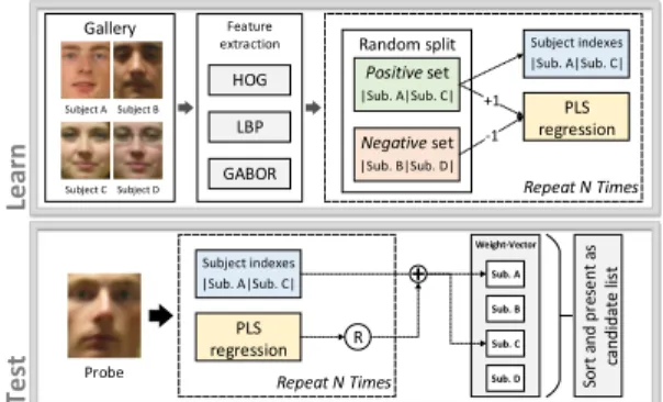
Le ar n Te st Feature extraction HOG LBP GABOR Gallery Subject C Subject D Subject B Subject A Repeat N Times Random split Positive set |Sub. A|Sub. C| Negative set |Sub. B|Sub. D| Subject indexes |Sub. A|Sub. C| PLS regression +1 -1 Weight-Vector Repeat N Times Subject indexes |Sub. A|Sub. C| PLS regression R Probe So rt an d p re se n t as can d id ate li st Sub. A Sub. D Sub. C Sub. B
Fig. 1: Overview of the proposed approach. During the learning step, different feature vectors are extracted and concatenated for each image in the face gallery. Then, several hash functions based on PLS models are learned using balanced random partitioning of subjects in the gallery in two subsets: positive and negative. Then, during test, we extract the same feature descriptors from the probe image and project them onto each PLS model to obtain a score value r, which is used to increase weights of subjects in the positive set (r may be negative, in which case votes are decreased). Finally, the list of subjects is sorted in decreasing order of weight and presented as candidates for identification.
discard the majority of subjects in the initial steps of the test using low computational cost weak classifiers.
Different from the aforementioned methods, the approach proposed in this work considers the benefits of LSH. In this context, our approach is more similar to [2], which uses random regression vectors to hash faces. However, instead of building random regressions, we consider PLS models inspired by the LSH principles presented in [14]: (i) data dependent hash functions and (ii) hash functions generated independently. The advantage of using PLS is that we can use combination of features in a high dimensional descriptor vector to achieve higher recognition rates [3].
III. PROPOSEDAPPROACH
The proposed method is inspired by two works in the literature: The first considers face identification based on large feature sets and PLS for simultaneous dimensionality reduction and classification [3], and the second based on independent hash functions [14]. An overview of the approach and a brief summary of its principles are presented in Figure 1. In the next sections, we explain Partial Least Squares for dimension reduction and regression (Section III-A) and the proposed hashing function based on PLS (Section III-B).
A. PLS regression and face identification
PLS is a statistical method composed of a dimensionality reduction step followed by a regression step in the low dimen-sional space. Dimendimen-sionality reduction consists in determining latent variables as linear transformation of the original feature vectors and target values, then, ordinary least squares is used to predict target values using latent variables from feature vectors. The advantages of PLS for face identification are robustness to unbalanced classes and support for high dimensional feature vectors. These advantages are presented in [3] and [17] where one sample per subject in the gallery is available for training and where several feature descriptors are concatenated in order to account for weaknesses of single feature descriptors.
The relationship among feature descriptors and target
val-ues is given as X = T PT + E and Y = U QT + F ,
where Xn×d denotes a zero-mean feature descriptor matrix
with n samples and d dimensions, Yn denotes a zero-mean
target vector where each row yicorresponds to the i-th feature
vector xi of X. The matrices Tn×p and Un×p denotes latent
variables from feature vectors and target values, respectively.
The matrix Pp×d and the vector Q are loading matrices
similar to PCA transformations. Finally, E and F represent residuals. PLS algorithms compute P and Q such that the covariance between U and T is maximum. In order to compute PLS, we consider the NIPALS algorithm [18] which output a
weight matrix Wd×p= {w1, ..., wp} such that cov[(ti, ui)]2=
arg max|wi|=1[cov(xwi, y)]2. The regression vector β between
T and U is calculated using least squares according to β =
W (PTW )−1TTY . A PLS regression response ˆy for a probe
feature vector x is calculated according to ˆy = ¯y + βT(x − ¯x),
where ¯y and ¯x denotes average values of Y and elements of
X, respectively. A PLS model is then defined as the variables
required to estimate ˆy (β, ¯x and ¯y).
To evaluate the gain obtained by the proposed approach with a real face identification method, we consider the work based on PLS described in [3]. The face identification method consists in learning one PLS model for each subject in the gallery following a one-against-all classification scheme. In this context, target values are set to +1 if the sample refers to the subject being considered or −1 otherwise. During test, samples are presented to each PLS model and their identities are assigned to the subject in the gallery related to the PLS model with maximum regression response.
B. PLS hashing
The proposed approach is based on two principles: (i) hash functions that consider the distribution of the data (data depen-dent) and (ii) hash functions generated independently among each other. As discussed in [14], independently generated hash functions are desirable to achieve uniform distribution of data in the hash table. Both principles are achieved following the steps presented in Figure 1. In the next paragraphs, we provide theoretical support, details, and practical design of the approach.
The approach consists in two steps: learning and test. On learning, we randomly split subjects in the gallery in two subsets: positive and negative. The split is performed as follows. For each subject, we sample from a Bernoulli distribution with parameter p = 0.5 and associate the subject to the positive subset in case of “success”. Then, a PLS model is learned considering feature descriptors extracted from samples in the positive set with target values equal to +1 against samples in the negative set with target values equal to −1. This
process is repeated several times1. A hash models is defined
by a single PLS model and the subjects in the positive subset. In the test step, we extract the same feature descriptors employed on the training for the probe image and present them to each PLS model to obtain a regression value r. Then, we increase by r each position of a weight-vector (initially zero) according to the indexes of subjects in the positive subset
1We repeat 150 times on FERET and 10-35 on FRGC datasets. The number
of repetitions depends on dlog2(#subjects)e and the dataset difficulty.
Subject D code Subject C code Subject B code Subject A code 1 Hash function 2 Bit 1 Bit 2 0 N eg at iv e sub se t 0 1 P os it iv e sub se t 0 1 1 Hash function 1 0 P os it iv e sub se t N eg at iv e su bs et
Binary counting sequence
Subject D code Subject C code Subject B code Subject A code 0 1 1 Hash function 1 0 P os it iv e su bs et N eg at iv e sub se t 1 Hash function 2 0 Bit 1 Bit 2 0 1 N eg at iv e sub se t P os it iv e sub se t Random split
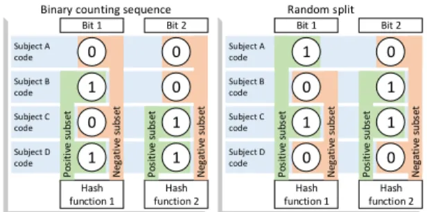
Fig. 2: Illustration of the importance to random split subjects. If codes follow a binary counting sequence (left), subsets are biased toward the order of subjects in the gallery and some possible configurations are lost (right). However, the performance of the proposed approach depends only on the capability of hash functions to distinguish between samples from subjects in the positive and negative subsets. of the same hash model. An advantage of such approach is that the average value of the weight-vector tends to zero when the number of subjects increase and, in practice, we can discard about half of the subjects that present negative values in the weight-vector since they rarely correspond to the correct subject.
The proposed weighted voting scheme differs from [14] in which compact binary hash codes are generated considering whether a sample falls in one or the other side of a maximum margin hyperplane. However, we achieved an increased accu-racy by employing the proposed weighted voting scheme in the face identification datasets in our experiments. The drawback is that the weighted voting scheme prevents the use of compact binary keys to index a hash table.
Instead of increasing positions in the weight-vector by r, we also tried to increase by a fixed value (say 1) if r > 0, however, this results in decreased accuracy. The intuition is that samples presenting positive r values closer to zero (samples that doubtfully belong to the positive subset) will be increased by the same amount as samples with r values close to +1 (more likely to be subjects in the positive subset). Moreover, we lose information regarding samples in the negative set when we do not decrement votes if r < 0. By increasing values in the weight-vector by r, we provide both more importance to samples with r values that indicate likely subjects in the positive set and decrement the importance of the same subjects when r indicate unlikely subjects. In addition, we also tried to model r using the cumulative logistic distribution and estimate the mean and standard deviation using 30 test samples, but the accuracy is also decreased.
To distribute subjects uniformly in the hash table, it is nec-essary to estimate the parameter p of the Bernoulli distribution. Consider that we assign a binary code for each subject, of a
total of N , in a gallery such that each code has log2(N ) = B
bits. We learn B hash functions to determine each bit of the code. The objective is to determine the probability of choosing
a bit b ∈ {0, 1} for a subject X = [x1, ..., xB] such that each
final binary code has equal probability, i.e,
P (code) = B Y i=1 P (xi= b) = 1 N, (1)
where xi is drawn independently and identically from a
Note that independence when drawing bits implies in independent hash functions. In the other hand, if we instead assign codes systematically among subjects, e.g., following a binary counting sequence (001, 010, ..., 111), the probability to assign a specific code to a subject will depend on codes already assigned to other subjects, breaking independence among the hash functions. If we systematically assign codes to subjects, we also limit the combinatorial number of binary subsets resulting in hash functions biased toward the order of codes assigned to subjects. Figure 2 illustrates the advantage of independent hash functions.
In practice, we learn more than B hash functions to reduce the number of collisions in the hash table when we independently draw bits from a probability distribution. We also expect that some hash functions will miss some bits (change one bit for another), However, considering unbiased classifier, it is expected a zero sum of r values from the missed bits such that the final result will be stable.
Considering the Bernoulli distribution, Equation 1 is rewrit-ten as
P (code) = pk(1 − p)B−k= 1
N, ∀k ∈ {0, ..., B}, (2)
where k is the number of bits in the code that are equal to 1. Expanding Equation 2, we have
P (code) = pB= pB−1(1 − p) = ... = (1 − p)B = 1
N, (3)
implying in p = 1 − p = 0.5. It can also be solved as
pB= 1
N =⇒ logp(
1
N) = log2(N ) =⇒ p = 0.5. (4)
It is possible to demonstrate that p = 0.5 minimizes the ex-pected number of collisions in the hash table. We experimented changing p to 0.3 and 0.7 and both values resulted in poor performance. Based on the aforementioned discussion, we can conclude that (i) the robustness of the hash functions depends on how well a classifier can distinguish between two random subsets of subjects, and (ii) each subset must hold half of the subjects.
IV. EXPERIMENTS
Herein we evaluate the proposed approach. In Section IV-A we describe general setup, such as the number of factors on PLS models and parameters regarding the feature descriptors considered. In Section IV-B, we evaluate feature combination, number of hash functions, stability, and results with face identification on FERET dataset, since it is the dataset with the highest number of subjects considered in our experiments. In Section IV-C, we evaluate the proposed approach on the FRGC dataset and compare with other methods in the literature. A. Experimental Setup
Feature descriptors considered are HOG, Gabor filters, and LBP. To computer Gabor features, we convolve the face image with squared filters of size 16 in 8 scales, equally distributed between [0, π/2], and 5 orientations, equally distributed be-tween [0, π], resulting in 40 convolved images. The convolved images are downscaled by a factor of 4 and concatenated to form the Gabor feature descriptors. Two feature descriptor
setups are used for HOG. The first consists in block size of 16 × 16 pixels with stride of 4 pixels and cell size equal to 4 pixels. The second consists in blocks of 32 × 32 pixels with stride of 8 pixels and cell size 8 pixels. For LBP, we consider the feature descriptor as the image resulted from the LBP transformation. The final feature vector is computed by concatenating features from the two HOG setups, Gabor and regular LBP applied to the image. The size of the final feature vector is 93,196.
The only parameter to build the PLS models is the number of factors (number of dimensions of the generated latent subspace). We tested varying the number of factors between 10 and 20 on FERET but the result was similar for any number of factors. Therefore, we consider 20 factors in all experiments.
All experiments were conducted on an Intel Xeon W3550 processor, 3.07 GHz with 64 GB of RAM running Fedora 16 operating system. All tests were performed using a single CPU core and no more than 8 GB of RAM were required during learn or test.
B. Results on the FERET dataset
The FERET [19] contains 1196 subjects, each having one image for training, and four test sets designed to evaluate robustness to illumination change, facial expression and aging. The test sets are: fb, 1195 images taken with different expres-sions; fc, 194 images taken in different lightning conditions; dup1, 722 images taken between 1 minute and 1031 days after the training image; and dup2, which is a subset of dup1 with 234 images taken 18 months after the training image. All images are cropped in the face region and scaled to 128 × 128 pixels. We use images with corrected illumination using the self-quotient images (SQI) method [20] kindly provided by the authors of [3].
Since dup2 is considered the hardest test set of FERET, we use dup2 to evaluate the combination of features, the stability, and the number of hash functions of the proposed approach. To isolate errors of the proposed approach from errors of the face identification, the plots are presented as the maximum achiev-able recognition rate, which is calculated considering that a perfect face identification method is employed for different percentages of candidates visited in the list. Preferable results present high maximum achievable recognition rate and low percentage of candidates visited, which, in general, represent curves close to the upper left corner of the plots. Finally, we evaluate the proposed approach on all four test sets from FERET dataset considering the face identification approach in [3].
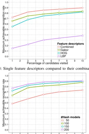
Feature combination. To assess that different feature descrip-tors contribute to better accuracy of the hash functions, we present, in Figure 3, the maximum achievable recognition rate when providing different percentage of the candidate list to the face identification. According to the results, the feature com-bination enhances the recognition rate for about 9% compared to the best single features (Gabor feature descriptors). Number of hash functions. Figure 4 shows the maximum recognition rate achievable for 50,100,150, and 200 hash func-tions. Significant improvement is achieved from 50 to 100 and from 100 to 150 hash functions. However, small improvement
0.0 0.1 0.2 0.3 0.4 0.5 0.6 0.7 0.8 0.9 1.0 1 2 3 4 5 6 7 8 9 10
Percentage of candidates visited
Maximum achievable recognition rate
Feature descriptors
Combined Gabor HOG LBP
Fig. 3: Single feature descriptors compared to their combination.
0.0 0.1 0.2 0.3 0.4 0.5 0.6 0.7 0.8 0.9 1.0 1 2 3 4 5 6 7 8 9 10
Percentage of candidates visited
Maximum achievable recognition rate
#Hash models
50 100 150 200
Fig. 4: Results for different numbers of hash functions. is noticed from 150 to 200. Therefore, we consider 150 hash functions on the remaining experiments. The average time to test each hash function is 250µs. Even though the theoretical
number of hash functions for FERET is dlog2(1196)e = 11,
we have to learn more hash functions for dup2 since it is the hardest test set on FERET. For fb and fc, for instance, about 100 hash functions return the same result.
Stability of hash functions. We run the proposed method five times with different random partitions to evaluate the stability of the results. Figure 5 presents the mean and standard deviation of the results. The conclusion is that the performance is stable for different partitions.
Face identification. Finally, we evaluate the proposed ap-proach using the face identification method as described in [3] (brief summary in Section III-A). Two plots are presented: one with the maximum achievable recognition rate (Figure 6a), and one with rank-1 recognition rates achieved when presenting the candidate list to the face identification method (Figure 6b). We can see that only 7% of the candidate list is necessary to achieve at least 95% of the recognition rate obtained by scanning all subjects.
C. Results on FRGC dataset
We consider the 2D images from FRGC version 1 [21] to compare the proposed approach with other methods [3], [4]. FRGC is consists in 275 subjects and images presenting variation in illumination and facial expression. The images were cropped in the facial region in the size 138 × 160 pixels and scaled to 128 × 128. We follow the same protocol in [4],
Candidates (%) 1 3 5 7 10 Mean 0.722 0.791 0.835 0.860 0.889 St. Dev. 0.014 0.005 0.012 0.016 0.013 0.50 0.55 0.60 0.65 0.70 0.75 0.80 0.85 0.90 0.95 1.00 1 2 3 4 5 6 7 8 9 10
Percentage of candidates visited
Maximum achievable recognition rate
Fig. 5: Mean maximum achievable recognition rate when running the proposed approach five times.
where a percentage of samples for each subject is randomly selected for train and the remaining used for test. The process is repeated five times and the average and standard deviation of speedup and rank-1 recognition are reported.
To compare with the tree-based approach proposed in [3], we select the number of hash functions and the maximum number of candidates in the list such that the averaged rank-1 recognition rate is close to 95%. This is necessary so we can compare speedup between the approaches directly. We also consider the heuristic proposed in [3] to stop the search on the candidate list. For a short number of initial test samples (15), the candidate list is scanned and identification scores are computed. Then, for the remaining samples, we stop scanning the list when a score higher than the median value of the scores is reached.
Results are presented in Table I. It can be seen that 16× on average speedup can be achieved when 90% of samples are used for training. However, the speedup decreases when fewer samples are available for training because we have to increase either the number of hash functions or the maximum number of candidates searched in the list. The conclusion is that the performance of the proposed approach depends on a high number of samples for training. Since the proposed approach does not consider face identities, we can try to include additional samples for learning on future works. We believe that the speedup of the proposed approach compared to the tree-based approach [3] is related to the independence of the hash functions since both approaches build PLS models in a similar manner.
V. CONCLUSIONS
We proposed a novel approach for hashing faces based on LSH and PLS regression. The hash functions are learned considering balanced random partitions of subjects in the face gallery, which we demonstrated to be the best option to avoid collision between two subjects. The performance of the proposed approach is simplified to how well a classifier dis-tinguishes between two random subsets of subjects in the face gallery. To learn robust classifiers, we consider a combination of feature descriptors and PLS regression models, which are appropriated for high dimensional feature vectors. Finally, the proposed approach demonstrated weak performance when a reduced amount of samples is available for training.
0.50 0.55 0.60 0.65 0.70 0.75 0.80 0.85 0.90 0.95 1.00 1 2 3 4 5 6 7 8 9 10
Percentage of candidates visited
Maximum achievable recognition rate
Test set fb fc dup1 dup2 (a) 0.50 0.55 0.60 0.65 0.70 0.75 0.80 0.85 0.90 0.95 1.00 1 2 3 4 5 6 7 8 9 10
Percentage of candidates visited
R ank -1 r ecognition r at e Test set fb (97.65) fc (98.96) dup1 (86.98) dup2 (84.61) (b)
Fig. 6: (a) Maximum achievable recognition rate of the proposed approach. (b) Rank-1 recognition rate achieved when the candidate list is presented to the face identification method [3]. Rank-1 recognition rate for scanning all candidates is shown in parenthesis for each experiment.
Percentage of samples for training 90% 79% 68% 57% 35%
CRC [4] Speedup 1.58× 1.58× 1.60× 2.38× 3.35×
Rank-1 recognition rate 80.5% 77.7% 75.7% 71.3% 58.0%
Tree-based [3] Speedup 3.68× 3.64× 3.73× 3.72× 3.80×
Rank-1 recognition rate 94.3% 94.9% 94.3% 94.46% 94.46%
Proposed approach
Speedup (16.84 ± 1.56)× (7.30 ± 1.40)× (5.66 ± 0.41)× (3.42 ± 0.34)× (2.79 ± 0.11)×
Rank-1 recognition rate (96.5 ± 0.7)% (96.7 ± 1.6)% (93.4 ± 1.3)% (93.6 ± 0.5)% (93.3 ± 0.7)%
Number of hash functions 10 20 25 35 35
Max. candidates 3% 10% 13% 20% 30%
TABLE I: Comparison between the proposed approach and other approaches in the literature. Higher speedups are shown in bold.
ACKNOWLEDGMENTS
The authors would like to thank the Brazilian National Research Council – CNPq (Grants #487529/2013-8 and #477457/2013-4 ), CAPES (Grant STIC-AMSUD 001/2013), and the Minas Gerais Research Foundation - FAPEMIG (Grants APQ-00567-14 and CEX – APQ-03195-13). This work was partially supported by the STIC-AmSud program.
REFERENCES
[1] R. Chellappa, P. Sinha, and P. J. Phillips, “Face recognition by com-puters and humans,” Computer, vol. 43, no. 2, pp. 46–55, 2010. [2] Z. Zeng, T. Fang, S. Shah, and I. A. Kakadiaris, “Local feature hashing
for face recognition,” in Biometrics: Theory, Applications, and Systems. BTAS. IEEE 3rd Int. Conf. on, 2009, pp. 1–8.
[3] W. R. Schwartz, H. Guo, J. Choi, and L. S. Davis, “Face identification using large feature sets,” Image Processing, IEEE Trans. on, vol. 21, no. 4, pp. 2245–2255, 2012.
[4] Q. Yuan, A. Thangali, and S. Sclaroff, “Face identification by a cascade of rejection classifiers,” in Computer Vision and Pattern Recognition (CVPR) Workshops. IEEE Conference on, 2005, pp. 152–152. [5] R. Jafri and H. R. Arabnia, “A survey of face recognition techniques.”
Journal of Information Processing Systems, JIPS, vol. 5, no. 2, pp. 41–68, 2009.
[6] J.-K. K¨am¨ar¨ainen, A. Hadid, and M. Pietik¨ainen, “Local representation of facial features,” in Handbook of Face Recognition. Springer, 2011, pp. 79–108.
[7] S. H. Salah, H. Du, and N. Al-Jawad, “Fusing local binary patterns with wavelet features for ethnicity identification,” in Signal Image Process, IEEE Int. Conf. on, vol. 21, no. 5, 2013, pp. 416–422.
[8] S. Liao, A. K. Jain, and S. Z. Li, “Partial face recognition: Alignment-free approach,” Pattern Analysis and Machine Intelligence, IEEE Trans. on, vol. 35, no. 5, pp. 1193–1205, 2013.
[9] M. F. Valstar and M. Pantic, “Fully automatic recognition of the temporal phases of facial actions,” Systems, Man, and Cybernetics, Part B: Cybernetics, IEEE Trans. on, vol. 42, no. 1, pp. 28–43, 2012.
[10] J. Wright, A. Y. Yang, A. Ganesh, S. S. Sastry, and Y. Ma, “Robust face recognition via sparse representation,” Pattern Analysis and Machine Intelligence, IEEE Trans. on, vol. 31, no. 2, pp. 210–227, 2009. [11] W. Deng, J. Hu, and J. Guo, “Extended src: Undersampled face
recog-nition via intraclass variant dictionary,” Pattern Analysis and Machine Intelligence, IEEE Trans. on, vol. 34, no. 9, pp. 1864–1870, 2012. [12] ——, “In defense of sparsity based face recognition,” in Computer
Vision and Pattern Recognition (CVPR), IEEE Conf. on, 2013, pp. 399– 406.
[13] J. Wang, H. T. Shen, J. Song, and J. Ji, “Hashing for similarity search: A survey,” arXiv preprint arXiv:1408.2927, 2014.
[14] A. Joly and O. Buisson, “Random maximum margin hashing,” in
Computer Vision and Pattern Recognition (CVPR), IEEE Conf. on, 2011, pp. 873–880.
[15] O. Barkan, J. Weill, L. Wolf, and H. Aronowitz, “Fast high dimensional vector multiplication face recognition,” in Computer Vision (ICCV), IEEE Int. Conf. on, 2013, pp. 1960–1967.
[16] B. He, D. Xu, R. Nian, M. van Heeswijk, Q. Yu, Y. Miche, and A. Lendasse, “Fast face recognition via sparse coding and extreme learning machine,” Cognitive Computation, vol. 6, no. 2, pp. 264–277, 2014.
[17] G. Chiachia, A. Falcao, N. Pinto, A. Rocha, and D. Cox, “Learning person-specific representations from faces in the wild,” Information Forensics and Security, IEEE Trans. on, vol. 9, no. 12, pp. 2089–2099, 2014.
[18] H. Wold, “Partial least squares,” in Encyclopedia of Statistical Science, S. Kotz and N. Johnson, Eds. New York: Wiley, 1985, pp. 581–591. [19] P. J. Phillips, H. Moon, S. A. Rizvi, and P. J. Rauss, “The FERET evaluation methodology for face-recognition algorithms,” Pattern Anal-ysis and Machine Intelligence, IEEE Trans. on, vol. 22, no. 10, pp. 1090–1104, 2000.
[20] H. Wang, S. Z. Li, and Y. Wang, “Face recognition under varying lighting conditions using self quotient image,” in Automatic Face and Gesture Recognition. Proc. Sixth IEEE Int. Conf. on, 2004, pp. 819–824. [21] P. J. Phillips, P. J. Flynn, T. Scruggs, K. W. Bowyer, J. Chang, K. Hoffman, J. Marques, J. Min, and W. Worek, “Overview of the face recognition grand challenge,” in Computer vision and pattern recognition (CVPR). IEEE Conf. on, vol. 1, 2005, pp. 947–954.
![Fig. 6: (a) Maximum achievable recognition rate of the proposed approach. (b) Rank-1 recognition rate achieved when the candidate list is presented to the face identification method [3]](https://thumb-eu.123doks.com/thumbv2/123doknet/12456933.336703/7.918.137.796.80.323/maximum-achievable-recognition-proposed-recognition-candidate-presented-identification.webp)
