HAL Id: hal-02952651
https://hal.archives-ouvertes.fr/hal-02952651
Submitted on 29 Sep 2020
HAL is a multi-disciplinary open access
archive for the deposit and dissemination of
sci-entific research documents, whether they are
pub-lished or not. The documents may come from
teaching and research institutions in France or
abroad, or from public or private research centers.
L’archive ouverte pluridisciplinaire HAL, est
destinée au dépôt et à la diffusion de documents
scientifiques de niveau recherche, publiés ou non,
émanant des établissements d’enseignement et de
recherche français ou étrangers, des laboratoires
publics ou privés.
SPATIO-TEMPORAL OBJECT STABILITY FOR
MONITORING EVOLVING AREAS IN SATELLITE
IMAGE TIME SERIES
Caglayan Tuna, François Merciol, Sébastien Lefèvre
To cite this version:
Caglayan Tuna, François Merciol, Sébastien Lefèvre. SPATIO-TEMPORAL OBJECT STABILITY
FOR MONITORING EVOLVING AREAS IN SATELLITE IMAGE TIME SERIES. ISPRS (Virtual
Conference), Jun 2020, Nice, France. �hal-02952651�
SPATIO-TEMPORAL OBJECT STABILITY FOR MONITORING EVOLVING AREAS IN
SATELLITE IMAGE TIME SERIES
Caglayan Tuna, Franc¸ois Merciol, S´ebastien Lef`evre∗ Univ. Bretagne Sud, UMR 6074, IRISA, F-56000 Vannes, France
{caglayan.tuna, francois.merciol, sebastien.lefevre}@irisa.fr Commission II, ICWG II/III
KEY WORDS: Satellite Image Time Series, Component tree, Spatio-temporal stability, Intertidal zones, Flood mapping
ABSTRACT:
Monitoring observable processes in Satellite Image Time Series (SITS) is one of the crucial way to understand dynamics of our planet that is facing unexpected behaviors due to climate change. In this paper, we propose a novel method to assess the evolution of objects (and especially their surface) through time. To do so, we first build a space-time tree representation of image time series. The so-called space-time tree is a hierarchical representation of an image sequences into a nested set of nodes characterizing the observed regions at multiple spatial and temporal scales. Then, we measure for each node the spatial area occupied at each time sample, and we focus on its evolution through time. We thus define the spatio-temporal stability of each node. We use this attribute to identify and measure changing areas in a remotely-sensed scene. We illustrate the purpose of our method with some experiments in a coastal environment using Sentinel-2 images, and in a flood occurred area with Sentinel-1 images.
1. INTRODUCTION 1.1 Motivation
Due to the climate change, it is crucial to have information about earth dynamics regularly. For instance, sea level rise is changing rapidly and up to date information about our earth is required. Sea level change may be caused by flood or tide, and observation capability of coastal side is increasing with data availability (Salameh et al., 2019). Remote sensing images en-able us to observe our earth with improved technology. New satellite missions such as Sentinel provide effective temporal resolution with approximately 5 days revisit time.
Unsurprisingly, Satellite image time series (SITS) analysis con-tinues to gain popularity in the literature. Such data combine spatial and temporal dimensions and they can be used for many problems such as assessing the temporal evolution of phenom-ena or objects (M´eger et al., 2019). Supervised classification algorithms currently represent the state-of-the-art in automatic mapping and monitoring of our planet, e.g. with deep neural networks that have reached very good performances on some well-defined scenarios. However, due to the difficulty to col-lect training data for each time sample, these methods might look less appealing than unsupervised algorithms (Petitjean et al., 2012). Indeed, although there are several reference data provided by industrial or institutional players, such data remain very expensive and time-costly to produce. Accurate unsuper-vised methods are thus needed to understand our entire Earth without requirement of reference data.
1.2 Related work
This paper aims at assessing evolving objects or phenomena in an unsupervised fashion. More precisely, we consider two use cases where observation of water areas is crucial: tides in Sentinel-2 images and floods in Sentinel-1 images. To do so, we
∗
Corresponding author
propose a novel methodology relying on morphological hier-archies. In this section, we review some related works, from both an application and a methodological point of view. Tide and flood mapping. Monitoring natural disasters is an important task for post-disaster management. Flood is one of the most common disasters and it is necessary to distinguish changes related to water from the other changes in order to cor-rectly find affected regions. Another natural event caused by water activity occurs in intertidal zones. Both events result from water mobility. According to (Salameh et al., 2019), availabil-ity of multitemporal images can provide an optimal solution for beach topography monitoring.
On the tide observation side, a k-means clustering is used in (Soares et al., 2012) in order to monitor intertidal zones. As a postprocessing, the authors apply morphological filtering (clos-ing) to the SAR images. Their work relies on bitemporal ana-lysis, thus making a limited usage of the temporal informa-tion. Pixelwise monitoring of intertidal zones with multitem-poral Synthetic Aperture Radar (SAR) images is proposed in (Catalao, Nico, 2016) with a method to analyse pixelwise in-tensity variations. Although their method is promising, object-based analysis is known to be more efficient than pixel object-based analysis for wetland landscape applications (Berhane et al., 2018) . In (Gonc¸alves, Henriques, 2015), authors used optical airborne images to extract Digital Surface Model (DSM) from coastal areas. Nevertheless, such DSM are not always available. As far as flood detection is concerned, Synthetic Aperture Radar (SAR) is known to be a valuable data source (Martinis et al., 2015, Tang et al., 2018). The SAR backscatter depends on the physical properties of the objects and, since water is re-flecting less than other materials (Tang et al., 2018), it is a dis-criminative feature for water detection. Therefore, radiomet-ric thresholding of backscatters is known as an efficient way to extract water areas (Giustarini et al., 2013). However, such a method is very sensitive to noise and spatial regularization
thus appears as a relevant strategy to improve robustness. Re-cently, flood detection was addressed with hierarchical repres-entations (Tuna et al., 2019). A min-tree was used to find an op-timal threshold and extract water regions. Although threshold-ing is an effective method, it is strugglthreshold-ing when the scene in-cludes soil moistures. Computation of the Normalized Differ-ence Flood Index (NDFI) from SAR images was recently intro-duced in (Cian et al., 2018), but its effective usage requires long time series data. Our aim is to propose an unsupervised method that extracts continuous spatio-temporal information from SITS since water shows a highly active behavior.
Morphological hierarchies and stable features. We aim at proposing a new, unsupervised method which is able to con-duct an object-based analysis of the images in the temporal domain. Morphological hierarchies are multiscale representa-tions of an image that provide access to the objects it contains at various scales-of-interest. More specifically, the question of building a morphological hierarchy for modelling a time series was addressed in our previous work (Tuna et al., 2020). We have used a component tree to observe the spatial structures in the time domain through temporal connectivity. As a related object-based temporal analysis work, we can mention the use of Maximally Stable Extremal Region (MSER) for video se-quences in (Donoser et al., 2010). A similar methodology was used for real-time text detection in (G´omez, Karatzas, 2014). They did not use temporal connectivity, but instead built a hier-archical representation for each time sample. To monitor the temporal evolution, a graph-based hierarchical representation was also used in (Khiali et al., 2019). The authors built a graph from predefined objects and then analyzed the evolution of an object through time. They aim to find objects which share a similar evolution. We also focus on such evolution but propose to do so through the definition of a novel spatio-temporal stabil-ity measure computed from a morphological hierarchy. Indeed, during the last decades, morphological hierarchies have been used for many applications (see (Bosilj et al., 2018) for a recent survey). However, to the best of our knowledge, such a spatio-temporal attribute was never used jointly with a morphological hierarchy, while such a definition would allow us to rely on ef-ficient and scalable algorithms and process large satellite image time series.
1.3 Contributions
In this paper, we inspire from the MSER concept built through a component tree approach to measure the stability in the tem-poral domain. Our contributions are twofold: i) we propose a new attribute called spatio-temporal stability to describe the evolution of regions through time; ii) we demonstrate the prac-tical interest of this attribute for Earth Observation with two applications related to monitoring of water areas: flood map-ping from Sentinel-1 and intertidal monitoring with Sentinel-2. Let us emphasize that our method is unsupervised so it does not require training samples to learn the observed phenomena. Organization of our paper is as follows. Section 2 provides some brief information about morphological representations usually built from still images but recently extended to satellite image time series. The spatio-temporal stability attribute and its post-processing will be presented in Section 3. Experimental results will be discussed in Section 4, before we conclude our paper in Section 5.
2. TREE REPRESENTATION
We recall here how to build a morphological hierarchy, that rep-resents an image through a tree structure. Furthermore, we de-scribe the space-time tree model recently proposed in (Tuna et al., 2020) that we use to derive our spatio-temporal stability at-tribute.
2.1 Component tree
As a representative example of morphological hierarchies, we consider in this paper the component trees (a.k.a max and min-trees). They were introduced by (Jones, 1999) as hierarchical image representation structures based on connected compon-ents. A tree consist of vertices and edges such asT = (V, E). We recall here their definition using the following notations. LetI be a grayscale image defined on the domain Ω ∈ N2
and taking values inV , i.e. I : Ω ∈ N2
→ V ∈ Z, x 7→ I(x) = v, withx and v denoting respectively the 2D pixel coordinates and intensity. The multi-scale representation is built using success-ive thresholdings with a thresholdλ ∈ Z, the lower and upper threshold sets being defined as
[I ≤ λ] = {x ∈ Ω, I(x) ≤ λ} (1) [I ≥ λ] = {x ∈ Ω, I(x) ≥ λ} (2) whereλ is an intensity threshold taking values within the im-age intensity range.range of the imim-age intensity. From these lower and upper sets, it is possible to extract the set of connec-ted componentsC(I) (given a predefined connectivity, e.g. 4-or 8-connectivity in images). These components are also called as nodes, and the node set of a tree is the union of its compon-ents:
V (I) = [ ∀k,λ
Cλ(I)k (3)
whereC denotes a connected component, k its index in the level λ of the image I. For the sake of simplicity, we will omit k andI notations in the sequel. The tree is created by finding parent-child relationships of each node. The root is the only node which has no parent and it covers the whole image. Leaves of the component tree include maximum (i.e. brighter objects) or minimum (i.e. darker objects) values of the image, for the max-tree and min-tree respectively.
2.2 Space-time tree
While morphological hierarchies have been built from still im-ages for decades, their definition over spatio-temporal data such as satellite image time series is more recent. In (Tuna et al., 2020), several strategies to build such a hierarchy have been in-troduced, and we focus here on the space-time tree. It assumes the SITS being seen as a spatio-temporal cube, where the two usual spatial dimensions are completed by a third dimension related to time. From this cube it is possible to build a single treeT (I1, . . . , In) where n is the length of the time series. The nodes of this space-time tree contain elements from multiple time stamps (i.e. pixels from multiple images in the series). If we denote the time dimension as a subscript of a node Cλ,t, space-time tree nodes can be represented as union of connected components from each time stamp separately:
Cλ,t= Cλ,1∪ Cλ,2. . . ∪ Cλ,n. (4)
Figure 1 shows a space-time max-tree example with a simple 4 × 4 × 3 matrix and the 6-connectivity rule which is created
Figure 1. Space-time max-tree example (best seen in colors). by gathering the 4 spatial connectivity and the 1 temporal con-nectivity (i.e. two temporal neighbors, previous and next). Each color represents a specific image and each arrow shows one node of the tree. The 6-connectivity rule can be formulated as
N6(x) = {(x′, t′) 6= (x, t) | max(|x − x′|, |t − t′
|) = 1} (5) It should be noted that, if a pixel faces some intensity change in the series (i.e.Ii(x) 6= Ii+1(x)), there will be no temporal con-nectivity and thus will result in two different nodes in the tree. We recall the root of the tree covers the whole time series and includes all three images. We can see that some nodes include pixels from every image/date, while some others include pixels from only one. Additionally, a real (but still simple) example is provided in Figure 2. We selected a few nodes from the whole tree for the sake of visualization. As we can see, such a model allows us to deal with spatio-temporal patterns present in the satellite image time series.
3. METHOD
We now explain how we build the spatio-temporal stability at-tribute from the tree. Then, we will use this atat-tribute to select some specific nodes of interest in the tree. Finally, an optional step consisting of area filtering will be discussed.
3.1 Spatio-Temporal Stability
As already stated, we propose to extend the stability concept used in the famous MSER method to deal with the temporal di-mension. Thus, we define the spatio-temporal stability of each node from the area ratio of the successive connected compon-ents though time. Here the area refers to the amount of pixels
in the node (Marcotegui et al., 2017) and we denote area of a node asA(C). We formulate the stability attribute St as
St(Cλ) = 1 n − 1 n−1 X i=1 min(A(Cλ,i), A(Cλ,i+1)) max(A(Cλ,i), A(Cλ,i+1)) (6) whereA represents the area attribute of the relevant C. The root node covers the whole spatial support all along the time series and thus has a spatio-temporal stability of1 independently of the lengthn of the series.
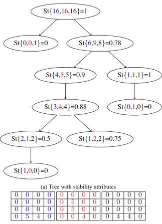
Figure 3 illustrates the spatio-temporal stability attribute of the nodes from the Figure 2. For each node of the tree, we provide the area occupied at each given time sample, as well as the spatio-temporal stability. Spatio-temporal stability attribute of the root node equals1 as expected. As we mentioned before, some nodes may cover a single date, thus have a null area in the other images. We set the stability attribute to0 for these nodes. 3.2 Node Selection
The stability measure can then be used to identify evolving or non-evolving objects in SITS. One way to extract information from trees is filtering. Filtering a tree consists in pruning the nodes according to some predefined criteria, usually by com-paring node attributes to some threshold. If our interest relates to evolving or unstable objects, nodes with low stability will be sought. To do so, we first retain all nodes having a stability lower than a given thresholdh. We then assign each pixel to the level of the node that is closest to the root (i.e. with the lowest λ value in case of a max-tree) to build the reconstructed image I′
:
I′(x) = min(λ | x ∈ Cλ(I), St(Cλ(I)) ≤ h) (7) and we set remaining pixels to 0. Let us note that a first pruning step is systematically applied to remove all nodes with stability equal to 0, that correspond to noisy regions appearing at a single time stamp.
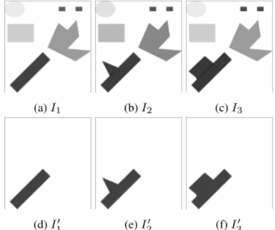
To illustrate, let us consider the tree in Figure 3a. Since we aim to find unstable regions, we should select some relatively low threshold, e.g.,h = 0.5. We then reconstruct the image (Fig. 3b) as usually done with tree-based filtering approaches. An additional example is provided in Figure 4 to show the be-havior of our approach. We can see a series of synthetic images with intensities that evolve through time together with the result of unstable region detection (or stable regions filtering). As we can notice, the spatio-temporal stability allows us to distinguish changing objects and static ones despite of intensity variations. We used the same threshold valueh = 0.5.
4. EXPERIMENTS
To illustrate the practical interest of our method, we have con-ducted two sets of experiments. The first aims to detect floods in Sentinel-1 SITS, while the second is focused on intertidal monitoring in Sentinel-2 SITS.
4.1 Flood mapping from Sentinel-1
For this first use case, we consider a series of Sentinel-1A im-ages acquired over Montmirail, North of France and East of Paris. More precisely, the data in use come with a spatial resol-ution of 10m, and consists in Ground Range Detected products
Figure 2. Space-time max-tree example built from real remote sensing data. The tree is built with 3 images and nodes include up to three images. St{16,16,16}=1 St{0,0,1}=0 St{6,9,8}=0.78 St{4,5,5}=0.9 St{3,4,4}=0.88 St{2,1,2}=0.5 St{1,0,0}=0 St{1,2,2}=0.75 St{1,1,1}=1 St{0,1,0}=0
(a) Tree with stability attributes
0 0 0 0 0 0 0 0 0 0 0 0 0 5 4 0 0 0 0 0 0 5 0 0 0 5 0 0 0 0 4 0 0 0 0 0 0 0 0 0 0 0 0 0 0 4 4 0
(b) Reconstructed images after filtering with spatio-temporal stability threshold h = 0.5.
Figure 3. Illustration of the spatio-temporal stability analysis of a space-time tree.
Image Acquisition Dates I1 17/07/2017 I2 10/08/2017 I3 25/01/2018
Table 1. Acquisition dates of Sentinel-1 images with the Interferometric Wide Swath (IW) and VV polarization. The SITS is made of 3 images (892×1941) as detailed in Table 1.
In order to assess the ability of our method to achieve flood detection, we use the Copernicus Emergency Management Ser-vice flood mapping1shape files as reference. A flooding event occurred on 22 January 2018, i.e. between second and third im-ages of the series, as shown in Figure 5. Flood mapping can be considered as a specific application of change detection fo-cused on water areas. So we compare the flooded scene with a non-flooded one (e.g. before the flood event) to identify among water regions those that are actually changing (i.e., floods) that we distinguish from water bodies. We then end with the fol-lowing difference image (wherei is the time when flooding is visible): If i = I ′ i− I ′ i−1 (8)
Since constant waters have the same location in successive im-ages, they are removed in If
. Finally, build a binary map through a simple threshold that discard null values:
If = (
255 Iif > 0
0 otherwise (9)
After finding the unstable nodes with a threshold empirically set toh = 0.2, some artifacts can remain (Cian et al., 2018) due to the double bounce effect, the backscatter similarity of dry soil, etc. In order to overcome these small errors, we post-process
Method F1 Proposed 0.78 (Tuna et al., 2019) 0.73 (Cian et al., 2018) 0.60
Table 2. Quantitative evaluation of flood detection results for different methods using theF1measure.
the binary change detection mapIf
with a small area filtering (i.e., with an area thresholdha= 20).
We report in Table 2 some quantitative evaluation obtained with theF1 score, i.e. the harmonic mean of precision and recall measures, defined as2 TP/(2 TP + FP + FN)) where TP are true positives (i.e., flooded pixels that were correctly detected by the method), FPs false positives (i.e., non-flooded regions detected as flooded) and FNs false negatives (i.e. flooded re-gions that have not been detected). We compare our results with those provided by two existing methods: the min-tree based ra-diometric thresholding (Tuna et al., 2019) that also relies on spatial attributes extracted from morphological hierarchies, and the Normalized Difference Flood Index (NDFI) (Cian et al., 2018) thresholding approach.
Figure 5 illustrates the original SITS (a-c) and the reference data (d), as well as the results obtained by the different methods (e-g): NDFI (Indf i), min-tree based radiometric thresholding (Tuna et al., 2019) (Imin) and our proposed method (If). To ease visual assessment, flooded areas are given using the fol-lowing color codes: TPs in green, FNs in red, and FPs in yel-low. We also provide some close-up illustrations. We can see from both Figure 5 and Table 2 that our method outperforms existing ones. (a) I1 (b) I2 (c) I3 (d) I′ 1 (e) I ′ 2 (f) I ′ 3
Figure 4. Synthetic example with input (top) and reconstructed (bottom) images.
4.2 Intertidal monitoring with Sentinel-2
We used Sentinel-2 images around Morbihan, France. Morbi-han and the Brittany region are well-known for their high tide behaviours. We limit ourselves to a sample SITS made of small extracts (632 × 927px) to ease visualization, considering 5 im-ages which were acquired in 2018 with a spatial resolution of 10m. We selected only cloud-free images in this illustrative ex-ample. We used level 2A products provided by the THEIA land data center2. Since there is no ground truth data for this ap-plication, we only report some visual assessment of our results. Acquisition dates of these images are given in Table 3. Since
2https://www.theia-land.fr/en/satellite-data/
Image Acquisition Dates I1 01/06/2018 I2 01/07/2018 I3 06/07/2018 I4 11/07/2018 I5 31/07/2018
Table 3. Acquisition dates of Sentinel-2 Images our focus in this paper is on the spatio-temporal nature of the data, we simplify each multispectral image into a grayscale one by computing the Normalized Difference Water Index (NDWI) (McFeeters, 1996) for each pixel. We recall that NDWI can be calculated from green (G) and near-infrared (NIR) bands of an image asN DW I = (G − N IR)/(G + N IR). Since water pixels appear brighter than other classes on the NDWI image, we used the max-tree for this experiment.
Figure 6 illustrates our experiments with Sentinel-2 images. Original images can be seen in the first row. We set the spatio-temporal stability of each pixel according to the stability of the deepest nodes they belong to (i.e., the one with the highest in-tensity value). More explicitly, water areas show higher val-ues than the other parts of the images. We provide the spatio-temporal stability imagesIst
i in the second row. The third row is the result obtained after filtering the space-time tree nodes with a spatio-temporal stability threshold empirically set toh = 0.4 and reconstructing the filtered SITS. We can notice some over-lap between the detected regions and the water regions visible in the original images. As expected, no land or sand region are de-tected by our method. For instance,I3shows some sandy areas on the water at the top left of the image and this is not detected as water inI′
3. We have also added a red rectangle inI′ 3, to em-phasize where the temporal connectivity has helped to ensure a correct detection. Although there is a gap in the spatial domain, this region still belongs to a node with high stability thanks to the successive images. Another red rectangle is given forI′
5. This part is dramatically growing at that time and correctly de-tected as an intertidal area with our method. Even if there is no temporal relationship, water pixels are connected in the spatial domain. For the sake of comparison, we provide in the last row the result of a pixel-based variation analysisIvar
obtained with the method from (Catalao, Nico, 2016). We can see in this last image that the tide areas are detected but the method does not provide a result per date. Besides, there are wrongly detected areas caused by intensity changes though time.
5. CONCLUSION
In this paper, we have introduced a new spatio-temporal stabil-ity attribute that can be efficiently measured from a space-time tree, i.e. a multiscale, hierarchical representation of a satellite image time series. This attribute relies on size variability of the tree nodes in the temporal domain. We used this attribute to monitor dynamic water regions such as floods in Sentinel-1 and intertidal zones in Sentinel-2. Since component trees are limited to analyze objects that are brighter or darker than their surroundings, future work will include using this attribute with other morphological hierarchies (e.g. tree of shapes, multiscale segmentations).
ACKNOWLEDGMENTS
The authors acknowledge the support of Centre National d’ ´Etudes Spatiales (CNES) and Collecte Localisation
Satel-lites (CLS), ANR under reference ANR-18-CE23-0022 (MULTISCALE project).
REFERENCES
Berhane, T. M., Lane, C. R., Wu, Q., Anenkhonov, O. A., Chepinoga, V. V., Autrey, B. C., Liu, H., 2018. Compar-ing pixel-and object-based approaches in effectively classifyCompar-ing wetland-dominated landscapes. Remote sensing, 10(1), 46. Bosilj, P., Kijak, E., Lef`evre, S., 2018. Partition and inclu-sion hierarchies of images: A comprehensive survey. Journal of Imaging, 4(2), 33.
Catalao, J., Nico, G., 2016. Multitemporal backscattering lo-gistic analysis for intertidal bathymetry. IEEE TGRS, 55(2), 1066–1073.
Cian, F., Marconcini, M., Ceccato, P., 2018. Normalized Dif-ference Flood Index for rapid flood mapping: Taking advantage of EO big data. Remote Sensing of Environment, 209, 712–730. Donoser, M., Riemenschneider, H., Bischof, H., 2010. Shape guided maximally stable extremal region (mser) tracking. 20th ICPR, IEEE, 1800–1803.
Giustarini, L., Hostache, R., Matgen, P., Schumann, G., Bates, P., Mason, D., 2013. A change detection approach to flood mapping in urban areas using TerraSAR-X. IEEE TGRS, 51(4), 2417–2430.
G´omez, L., Karatzas, D., 2014. Mser-based real-time text de-tection and tracking. 22nd ICPR, IEEE, 3110–3115.
Gonc¸alves, J., Henriques, R., 2015. UAV photogrammetry for topographic monitoring of coastal areas. ISPRS Journal of Pho-togrammetry and Remote Sensing, 104, 101–111.
Jones, R., 1999. Connected filtering and segmentation using component trees. Computer Vision and Image Understanding, 75(3), 215–228.
Khiali, L., Ndiath, M., Alleaume, S., Ienco, D., Ose, K., Teis-seire, M., 2019. Detection of spatio-temporal evolutions on multi-annual satellite image time series: A clustering based approach. International Journal of Applied Earth Observation and Geoinformation, 74, 103–119.
Marcotegui, B., Serna, A., Hern´andez, J., 2017. Ultimate open-ing combined with area stability applied to urban scenes. In-ternational Symposium on Mathematical Morphology and Its Applications to Signal and Image Processing, Springer, 261– 268.
Martinis, S., Fissmer, B., Rieke, C., 2015. Time series analysis of multi-frequency SAR backscatter and bistatic coherence in the context of flood mapping. MultiTemp.
McFeeters, S. K., 1996. The use of the Normalized Difference Water Index (NDWI) in the delineation of open water features. International journal of Remote Sensing, 17(7), 1425–1432. M´eger, N., Rigotti, C., Pothier, C., Nguyen, T., Lodge, F., Gueguen, L., Andr´eoli, R., Doin, M.-P., Datcu, M., 2019. Rank-ing evolution maps for Satellite Image Time Series exploration: application to crustal deformation and environmental monitor-ing. Data Mining and Knowledge Discovery, 33(1), 131–167.
Petitjean, F., Inglada, J., Ganc¸arski, P., 2012. Satellite image time series analysis under time warping. IEEE TGRS, 50(8), 3081–3095.
Salameh, E., Frappart, F., Almar, R., Baptista, P., Heyg-ster, G., Lubac, B., Raucoules, D., Almeida, L. P., Bergsma, E. W., Capo, S. et al., 2019. Monitoring Beach Topography and Nearshore Bathymetry Using Spaceborne Remote Sensing: A Review. Remote Sensing, 11(19), 2212.
Soares, F., Catalao, J., Nico, G., 2012. Using k-means and mor-phological segmentation for intertidal flats recognition. IEEE IGARSS, 764–767.
Tang, D., Wang, F., Xiang, Y., You, H., Kang, W., 2018. Auto-matic water detection method in flooding area for gf-3 single-polarization data. IEEE IGARSS, 5266–5269.
Tuna, C., Merciol, F., Lef`evre, S., 2019. Analysis of min-trees over sentinel-1 time series for flood detection. MultiTemp, IEEE, 1–4.
Tuna, C., Mirmahboub, B., Merciol, F., Lef`evre, S., 2020. Com-ponent trees for image sequences and streams. Pattern Recog-nition Letters, 129, 255–262.
(a) I1 (b) I2 (c) I3
(d) Iref
(e) Indf i
(f) Imin
(g) If
Figure 5. Flood Observation (from top to bottom): Original Sentinel-1 images (a)-(c); Reference image for flood (d); Results with NDFI (e), the min-tree threshold analysis (f), and our method (g). Results are given in green, red, and yellow for TP, FN, and FP
(a) I1 (b) I2 (c) I3 (d) I4 (e) I5 (f) Ist 1 (g) I2st (h) I3st (i) I4st (j) I5st (k) I1′ (l) I ′ 2 (m) I ′ 3 (n) I ′ 4 (o) I ′ 5 (p) Ivar
Figure 6. Intertidal Observation. a-e: Input Sentinel-2 NDWI images; f-j: Stability feature image for each time sample; k-o: Tide Observation for each time sample with our method; p: Tide observation with the pixelwise variation method.