O
pen
A
rchive
T
OULOUSE
A
rchive
O
uverte (
OATAO
)
OATAO is an open access repository that collects the work of Toulouse researchers and
makes it freely available over the web where possible.
This is an author-deposited version published in :
http://oatao.univ-toulouse.fr/
Eprints ID : 17206
The contribution was presented at SBAC-PAD 2016 :
http://www2.sbc.org.br/sbac/2016/
To cite this version :
Villebonnet, Violaine and Da Costa, Georges and
Lefèvre, Laurent and Pierson, Jean-Marc and Stolf, Patricia Energy Aware
Dynamic Provisioning for Heterogeneous Data Centers. (2016) In: 28th
International Symposium on Computer Architecture and High
Performance Computing (SBAC-PAD 2016), 26 October 2016 - 28
October 2016 (Los Angeles, United States).
Any correspondence concerning this service should be sent to the repository
administrator:
[email protected]
Energy Aware Dynamic Provisioning
for Heterogeneous Data Centers
Violaine Villebonnet
∗†, Georges Da Costa
∗, Laurent Lefevre
†, Jean-Marc Pierson
∗and Patricia Stolf
∗∗IRIT, University of Toulouse, France
†Inria Avalon LIP - Ecole Normale Superieure of Lyon, University of Lyon, France
Abstract—The huge amount of energy consumed by data centers represents a limiting factor in their operation. Many of these infrastructures are over-provisioned, thus a significant portion of this energy is consumed by inactive servers staying powered on even if the load is low. Although servers have become more energy-efficient over time, their idle power consumption remains still high. To tackle this issue, we consider a data center with an heterogeneous infrastructure composed of different machine types – from low power processors to classical powerful servers – in order to enhance its energy proportionality. We develop a dynamic provisioning algorithm which takes into account the various characteristics of the architectures composing the infrastructure: their performance, energy consumption and on/off reactivity. Based on future load information, it makes intelligent decisions of resource reconfiguration that impact the infrastructure at multiple terms. Our algorithm is reactive to load evolutions and is able to respect a perfect Quality of Service (QoS) while being energy-efficient. We evaluate our original approach with profiling data from real hardware and the experiments show that our dynamic provisioning brings significant energy savings compared to classical data centers operation.
I. INTRODUCTION
Large scale data centers are most of the time dimensioned by conception, and they are often over-provisioned, especially if they provide services with high quality constraints. This implies that energy is consumed to maintain servers on for potential future demand, but in reality these servers are staying inactive. To address this issue, many works around dynamic provisioning and capacity planning propose to turn off unused servers and turn them on only when they are needed, thus save important amounts of energy.
Another conception problem concerns the servers them-selves and their power consumption curve. Some studies [1], [2] have shown that the power consumed by an idle server can represent up to 50% of its peak power consumption, resulting in high static costs. Recently, some mobile processors achieve a more proportional power curve as their idle consumption is very close to zero. Unfortunately, their performance is still poor compared to powerful servers. It has been demonstrated that bringing different types of architecture into a unique heterogeneous data center allows to enhance energy efficiency and energy proportionality [3].
In our previous work, we have proposed the ”Big, Medium, Little” (BML) infrastructure [4] composed of several types of machines with various performances and energy con-sumptions. This heterogeneity brings a way to adapt more precisely the infrastructure and its consumption to the actual
load. However, our observation is that these architectures also have very different characteristics in terms of switch on/off reactivity and energy overheads, which need to be considered when making reconfigurations decisions. This is why in this work, we propose a more complex dynamic provisioning algorithm of bare-metal resources, adapted to heterogeneous infrastructures. It takes into account the different temporal effects of switch off against switch on actions, as well as their various durations depending on the architectures. It takes both load-reactive and energy-saving actions in order to process all incoming workload while being energy-aware. This approach is generic and can be used with many architecture types.
This paper is organized as follows: Section II presents some related works on resource dynamic provisioning. The algorithm specifications are presented in section III while the algorithm itself is detailed in section IV. Section V contains experiments and validations considering a scenario with stateless web servers. Section VI concludes and presents some future works.
II. RELATEDWORK ONDYNAMICPROVISIONING
Dynamic provisioning is a resource management technique consisting in powering on the minimum quantity of servers necessary to meet the current demand, while balancing the load among them. By essence, this approach allows to enhance the energy proportionality of a data center as its composition is dynamically adapted to the load fluctuations. Many works have been undertaken around this topic. In one of the earliest, Pinheiro et al. have proved with simple experiments the potential energy savings of dynamic against static provisioning for a small homogeneous cluster of 8 servers [5].
Several works have followed and proposed new methodolo-gies to improve the techniques by focusing on specific aspects. In [6], Chen et al. studied the performance impacts of dynamic provisioning in different scenarios: with and without load forecasting, and with two different implementations of load dispatching. Lin et al. [7] have proposed the term ”dynamic
right-sizing”, and defined an algorithm named LCP for Lazy Capacity Provisioning. The authors have precisely evaluated its achievable energy gains against an optimal offline version. Despite their work being very thorough, it stays at a theoretical level as they have made important assumptions about power model: considering that a server consumes a fixes amount of energy when processing any load level, and making an approximative definition of the switching overheads.
All the above-cited works only apply to homogeneous data center configurations. We believe that including different types of servers in a data center infrastructure brings some interest-ing features that can be exploited to enhance the relevance of dynamic provisioning. To the best of our knowledge, no existing works have taken into account the different tempo-ralities of the switch on and off actions of heterogeneous machines like we propose in this paper. However, some works do consider dynamic provisioning at different time scales. This has been enabled by virtualization technologies as deploying a virtual machine has a shorter duration that turning on a machine. For instance, Ardagna et al. [8] have focused on web services placement across multiple geographically distributed cloud sites. They have defined two types of actions: resource provisioning at mid-long term across different sites, and virtual machine provisioning inside a same site at short term. Though in our work we are considering different time scales for reconfigurations, we apply it to heterogeneous bare-metal resource provisioning.
III. ALGORITHMSPECIFICATIONS
Through this section we highlight the goals of our algorithm by describing the specifications of the problem we consider:
• Multiple-term reconfiguration decisions:
Reconfiguration actions of computing resources do not affect the infrastructure at the same speed. On one hand, switching off a machine has an immediate impact: as soon as the power-off decision is made, the server starts its shut-down process and is no longer available for computing. On the other hand, switching on a machine takes some time before the machine is actually on and ready to compute. Moreover, according to the architecture type, switch-on actions can have very different durations. Hence, our algorithm takes this into account and is able to make decisions of reconfigurations which have multiple-term effects: either at immediate-, short- or long-term. • Generic in terms of architecture types and quantity: We design our algorithm for heterogeneous infrastructures, that is why genericity is an essential feature. It is important that our work is adapted to different quantities of architecture types, as well as their various characteristics. For instance, no modification of the algorithm is needed neither if we have a homogeneous cluster, nor if the cluster is highly heteroge-neous. Also, we make no assumptions on the machine profiles, and we evaluate our work with data acquired experimentally on real hardware in section V.
• Dynamic and reactive to workload evolution: We target applications with variable load and we aim at adapting the infrastructure to load conditions so that the energy consumption more closely matches resource utilization. However, we do not want to reduce consumption at the expense of performance, and we consider a maximum quality of service (QoS) requirement in our work. For this purpose, our algorithm reacts to load evolutions by dynamically taking provisioning decisions so that the perfect QoS is respected.
• Energy-proportional-aware:
The principal goal of dynamic provisioning is to save energy by turning off unused servers during periods of low loads. As just described, our algorithm is designed to react to load evolutions. This may sometimes result in situations where the infrastructure has the right capacity to process the current load, but the composition of the powered on machines may not be the most energy efficient. If such conditions occur, the algorithm decides to reconfigure the infrastructure towards the ideally energy proportional composition for the predicted load.
IV. ALGORITHMDESCRIPTION
A. Prerequisites
1) Performance and Energy Profiling:
A profiling phase is necessary to characterize the behavior of all types of machine in terms of performance and energy consumption. In this phase, we need to determine the max-imum performance rate that each type of architecture can reach when running the target application, and what energy it consumes both at maximum performance and in idle state. Another essential information we need to know is the durations of switch on and off for each machine type, as well as the energy consumed during these actions.
Here is a summary of the data we acquire during the profil-ing phase, with their notation and definition. LetM be the set of architectures composing our heterogeneous infrastructure. For each architecturei ∈ M, we collect from profiling:
• perfmaxi: maximum performance rate reached by archi-tecturei. It must be characterized using an application
metricthat represents the amount of work performed over a given time step denoted ∆t. Such a metric is used to assess the application performance independent of the underlying architecture. Further in Section V, we use as metric the number of requests processed per second by a web server, but for example it can also be frame rate for video rendering, and so on.
• emaxi: energy consumed by architecture i during one time step ∆t when achieving perfmaxi, expressed in Joules.
• poweridlei: average power consumed by architecturei in idle state, expressed in Watts.
• tOni: time required to power on architecturei, expressed in seconds.
• tOf fi: time required to power off architecturei, expressed in seconds.
• eOni: energy consumed during the power-on period of architecturei, expressed in Joules.
• eOf fi: energy consumed during the shut-down period of architecturei, expressed in Joules.
2) Ideal Combinations and Utilisation Thresholds:
Once all machine profiles are built, a computational phase is conducted to determine the most energy-proportional com-binations of architectures for all possible performance rates. First, this process starts by sorting architectures regarding their
maximum performance perfmaxi. Then, it checks that their respective maximum energy consumption emaxi follow this initial ordering. We proceed by comparing sorted architectures in pairs; if an architecture has lower performance than another while consuming more energy, we remove it from the archi-tecture setM as it does not respect the required properties to improve energy proportionality.
After this sorting, the next step establishes how chosen architectures should be combined to create the most energy-proportional infrastructure. This consists in finding crossing points between machine profiles. These crossing points rep-resent the moment when it becomes more energy efficient to use a more powerful machine than using a combination of less powerful ones. Consequently, for each architecture i ∈ M, we denoteminT hreshithe minimum threshold of utilization of architecture i. This threshold is expressed regarding the chosen application metric. Additionally, we notemaxN bithe maximum number of machines of each architecture i that compose ideal combinations. For example, it can picture the fact that it is not ideally energy-efficient to use moremaxN bA machines, but instead use machines of typeB, sorted just after A in the set of architectures. As a result, we have at disposition a function able to compute the ideal combination of machines for a given performance rate.
Note that our approach is not constrained by the number of machines of each architecture type. We consider that enough machines of each type are available to choose from when building machine combinations. This enables to create ideal combinations based on hardware profiles. With minor changes, this work can consider cases where an heterogeneous infrastructure has already been established, and there are thus limited numbers of machines of each type.
3) Minimum Switching Interval:
We aim at saving energy by turning off unused machines, but we also want to respect maximum QoS requirements, that is why we need to power on machines perfectly in time to process the incoming workload. Moreover, these switch on and off actions represent energy overheads that we must consider. As a consequence, the decision of turning off a machine must be taken carefully, with knowledge that this machine will stay powered off for a certain minimum interval. We defineTi
s as the minimum amount of time for which it is more efficient to switch off machinei than to keep it powered on but idle. It is computed as follows: Ti s= max ( eOni + eOf fi poweridlei , tOni+ tOf fi ) This interval is inspired from the definition of Orgerie et
al. in [9], while assuming that POF F, the consumption of a machine when it is powered off, is equal to 0. We need to enhance the definition by adding the maximum function because with some low power processors we have profiled, it happens thattOn+tOf fis actually greater than the fraction in the first term of ourTs definition. In [10], Lu et al. describe
a similar concept, but in a more theoretical way, as∆ which they called ”critical time”.
B. Functioning of the Algorithm in details
Our algorithm is composed of two main categories of actions: (i) load-reactive actions and (ii) energy-saving actions, which put together translate into three different types of actions : Switch-On, Switch-Off, and Back-to-Ideal. The first two consist in actions of machines switch on or off, considered independently, while the last one considers all the powered-on machines as a combinatipowered-on and decides to recpowered-onfigure the infrastructure towards a more energy-efficient combination if possible. At each time step, the algorithm starts by proposing load-reactive actions. In case no reactive actions are needed, which means that the capacity of the current infrastructure composition is sufficient to process the incoming workload, the algorithm may propose an energy-saving action. We detail the implementation of all these reconfiguration decisions in the following explanations.
In our work, we assume that the data center operator – executing our dynamic provisioning algorithm – has complete knowledge of the workload ahead of time, and consequently, our algorithm will provision exactly to always satisfy the peak loads. As we want to take advantage of the different temporalities of the reconfigurations actions, the algorithm analyzes the future load knowledge via different look-ahead windows whose sizes are precisely chosen. We assume that we have at disposition a prediction function able to give the performance rate needed during a specific future load window. In our case, this function simply returns the maximum performance rate that will occur during this time slot. Of course, we can imagine that the knowledge of the future workload is in fact predicted upon historical data load.
Because our algorithm takes reconfiguration decisions that will take place at different moments in the future, we assume there is a system memorizing the decisions, therefore knowing at any moment what are the ongoing switch-on or off actions. Consequently, it is possible to compute the future processing capacity of the infrastructure knowing the current one and the ongoing actions.
1) Load-Reactive Actions:
At each time step, the algorithm proposes load-reactive actions. It tries to find what switch-on or -off actions are the most appropriate reactions to the incoming workload.
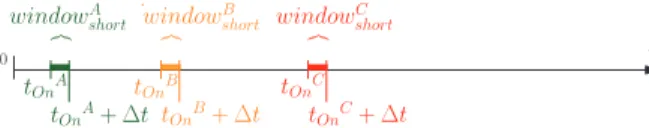
• Switch-On actions:
Let tnow denote current time. To decide if any switch-on actions are needed for machines of a given architecture i, the considered look-ahead window must start attnow+ tOni. Indeed, as machine of type i will take tOni seconds before being ready to compute, it is not necessary to look at future load before this point. As we want to avoid over-provisioning as much as possible, we decide to take one time step∆t as window length. For each architecturei, we note windowi
short its future load window used to decide switch-on actions.
t0 tOnA tOnA+∆t tOnB tOnC tOnB+∆t tOnC+∆t t windowC short windowB short windowA short z}|{ z}|{ z}|{
Fig. 1. Short look-ahead windows used for switch-on actions.
On Figure 1 are pictured the look-ahead windows for switch-on actions for an illustrative example of a data center containing three architecture types notedA, B and C. To ease the notations in the following and avoid repeating tnow, we consider thattnow= t0= 0.
We detail in the following the successive steps for the computation of the quantity of machines to switch on. We assume that we are not limited in the quantity of machines of each type. Because we want to respect the QoS, the algorithm makes the decision to switch on as many machines as needed to answer the predicted future load difference. But in order not to switch on all types of machines and thus results in an over-provisioned architecture, the decision to switch on some machines of architecturei is only taken if the predicted load difference is superior or equal to the minimum utilization thresholdminT hreshi of this architecture.
The decision process for Switch-On actions is as follows: For all architecture typesi ∈ M :
1) Compute the load prediction for windowi short. 2) Compute the maximum difference dif fi
short between the load prediction and the future capacity of the in-frastructure during the considered window.
3) If this difference is greater than or equal to the min-imum utilization threshold minT hreshi, it means that machines of typei need to be switched on; Compute the minimum quantity of machines i necessary to process the predicted load difference:
nbOni= ⌊ dif fi
short / perfmaxi ⌋
4) Else, no machine of type i needs to be switched on, nbOni= 0.
• Switch-Off actions:
Switch-off actions are also part of load-reactive actions because we want to shut down all machines becoming unnec-essary when the load decreases in order to save energy. We discussed the minimum switching intervalTi
s in the prerequi-sites, it justifies that the look-ahead windows must start from current timetnowand have a length ofTsi. Figure 2 illustrates these switch-off windows for illustrative architectures A, B andC, denoted windowi
immas they begin immediately in the future.
Switch-Off actions are decided as follows:
1) For all architecture typesi ∈ M whose current quantity of machines powered onnbiis positive; Propose switch-off actions:
a) Compute the load prediction forwindowi imm. b) Compute the maximum difference dif fi
imm be-tween the load prediction and the future capacity
t0 t TsA TsB TsC z }| { z }| { z }| { windowC imm windowB imm windowA imm
Fig. 2. Immediate look-ahead windows used for switch-off actions.
of the infrastructure during the considered window. c) If this difference is negative, meaning that the load is decreasing, compute the maximum quantity of machines of typei that can be turned off: nbOf fi= min(⌊ |dif fi
imm| / perfmaxi ⌋, nbiOn) d) Else, no machine of type i can be switched off,
nbOf fi= 0.
2) Compute all possible switch-off reconfigurations as the combinations of all proposed switch-off actions. 3) Remove the switch-off reconfigurations which do not
respect the QoS during their associatedwindowimm. 4) Sort the switch-off reconfigurations in the decreasing
order of their impact in term of processing capacity. 5) Choose the most appropriate switch-off reconfiguration:
a) For all switch-off combinations: If one of them allows to reconfigure the infrastructure towards an ideal combination for any windowi
imm, then perform this reconfiguration.
b) Else, perform the switch-off reconfiguration with the biggest impact in term of processing capacity.
2) Energy-Saving Actions: • Back-to-Ideal actions:
If no load-reactive actions have been proposed in the first phase of the algorithm, this second phase tries to propose an energy-saving action by reconfiguring the infrastructure to-wards an ideal and energy-efficient combination of machines. In fact, we consider as Back-to-Ideal action a reconfiguration which will turn off some (combination of) not energy-efficient machines and replace them by turning on some (combination of) more energy-efficient machines, according to the consid-ered future load. As those actions can consist in an important reconfiguration, we want to perform it only towards a quite stable situation, and only if the reconfiguration overhead is not too high. That is why we use long term look-ahead windows.
t0 t tOnA tOnB tOnC tOnC+TC s z }| { z }| { z }| { windowC long windowB long windowA long=windowM AX
We definewindowM AX as the maximum look-ahead win-dow used to decide energy-saving actions, and also used to check if the future load is globally increasing or decreasing. This window starts atmin(tOni) and ends at max(tOni+ Tsi). For all architectures i we note windowi
long the look-ahead window starting at tOni and ending like windowM AX at max(tOni+ Tsi). There are all represented on Figure 3, and we explain in the following their use in the algorithm.
The decision of Back-to-Ideal action is only taken if no load-reactive actions have been proposed, and if there are currently no other ongoing reconfigurations, i.e., switch on/off actions not yet completed. Of course, another prerequisite of performing such an action is that the current combination of machines should not already be an ideal combination for any of the look-ahead windows.
Assuming these conditions are fulfilled, there are two dif-ferent situations when a Back-to-Ideal action is needed: (i) The load decreases in the future, and the current combination is sufficient to process it, but is also over-provisioned in a way that it is not possible to turn off any machines because there are all utilized. (ii) The load increases in the future, meaning that we will need to turn on new machines but the current combination is already far from ideal considering energy consumption.
Here is the detailed process to decide a Back-to-Ideal action: 1) Compute the load prediction for windowM AX, and the reconfigurationreconf Ideal towards the associated ideal combination.
2) If the load prediction is lower than the processing capac-ity of the current infrastructure, the load is decreasing:
a) Compare all consecutivewindowi
longto assure that the load is monotonically decreasing. (Else, exit). b) Analyzereconf Ideal to know which architecture
mArch taking part in this reconfiguration has the maximum switch-on durationtmArch
On . c) If tmArch
On is different from min(tOni), it means that it is not optimal to perform the reconfiguration towards the ideal combination for windowM AX but instead windowmArch
long should be considered; Compute the load prediction onwindowmArch
long and updatereconf Ideal to the new associated recon-figuration. (Else, keep the previousreconf Ideal). d) Compute the energy overhead of the reconfigura-tion reconf Ideal: the sum of all Switch-On and Switch-Off energy overheads.
e) Compute the over-consumption due to staying in the current combination for the predicted load. f) If the overhead of the reconfiguration is lower than
the over-consumption of the current combination: Perform Switch-On actions ofreconf Ideal. (Else, exit).
3) Else, it means that the load prediction is greater than the processing capacity of the current infrastructure, hence the load is increasing:
a) Check if the current combination of machines is
already far from ideal; It consists in verifying that any quantity of machines of type i is greater than maxN bi. (Else, exit).
b) Compare all consecutivewindowi
longto assure that the load is monotonically increasing. (Else, exit). c) Same as Step 2) b).
d) Same as Step 2) c).
e) Perform Switch-On actions ofreconf Ideal. Note that we only perform the Switch-On actions of the chosen Back-to-Ideal because the switch-off actions will automatically be done later as a load-reactive action.
V. EXPERIMENTS ANDVALIDATIONS
A. Machine Profiling Results
Our chosen heterogeneous infrastructure is composed of three different architectures. We choose two ARM proces-sors, Cortex-A7 and Cortex-A15, provided by respectively a Raspberry Pi 2 Model B+, and a Samsung Chromebook. ARM processors consumes little energy when idle as they were originally designed for embedded devices where low power consumption results in extended battery life. Their performance has improved over time, resulting in several ARM server solutions for data centers, however, they are not yet as powerful as traditional servers. This motivated us to combine both low power processors and regular servers in our heteroge-neous infrastructure. We select a classical powerful server with an Intel Xeon processor, available at Grid’5000 [11]. It is a French experimental testbed dedicated to scientific research, where some clusters are equipped with power monitoring systems accessible via an API named Kwapi [12]. To monitor the energy consumption of the ARM machines, we use a Watts
Up? Prowatt-meter. The selected processors are:
- Big: x86 Intel Xeon E5-2630v3 (2 x 8 cores) - Medium: ARM Cortex-A15 (1 x 2 cores) - Little: ARM Cortex-A7 (1 x 4 cores)
A stateless web server is our target application because: • a load balancer could allow the load to be distributed
among several web server instances;
• being stateless, an application can be more easily mi-grated as migration consists in stopping a server instance and launching a new one on the destination machine, and then updating the load balancer;
• it is a representative example of an application whose load varies over time, and its performance can be characterized with a unique application metric, the number of requests processed per second.
We use lighttpd [13] as web server and siege [14] as web benchmark tool. The content of the profiled web server is a cgi script written in Python. Each request consists in a loop of random number generation. To craft requests of heterogeneous sizes, the number of loop iterations is also chosen randomly between 1000 and 2000. A response to a request consists in a static html page that contains the integer representing the number of iterations. For each architecture, we execute
the benchmark test with an increasing number of concurrent clients in order to find the maximum request rate that can be
processed per second, as the considered time step ∆t is one
second. Each benchmarking test runs for 30 seconds, and the maximum performance level is computed as the average of 5 benchmark results. The maximum energy consumption is also the average consumption of 5 executions. We evaluate the time to switch on and off each machine type, as well as the energy consumed during these actions. The results are presented in the first part of Table I, together with the durations in seconds of switch on and off actions, and their corresponding energy consumption in Joules. The values are averages of 5 measures for each action.
TABLE I
ARCHITECTURES PROFILES.
Acquired data Big Medium Little
perfmax(reqs/s) 1331 33 9
emax(J) 200.5 7.6 3.7 poweridle(W) 69.9 4 3.1 tOn(s) 189 12 16 tOf f (s) 10 21 14 eOn(J) 21341 49.3 40.5 eOf f(J) 657 77.6 36.2
Computed parameters Big Medium Little
Ts(s) 315 33 30
minT hresh (reqs/s) 529 10 1 maxN b ∞ 16 1
The second part of Table I contains the computed
pa-rameters (Section IV), that are: Ts the minimum switching
interval,minT hresh the minimum utilization threshold, and
maxN b the maximum number of machines from each type composing ideal combinations. From this Table we observe that the Little architecture has a very low range of utilization and that combinations should not contain more than one Little machine to be ideally energy-efficient. We will discuss this issue with the following results.
B. Simulation Setup and Temporal Visualisation
To evaluate our approach we developed a simulator in Python, which takes as inputs the experimental profiles pre-sented in Section V-A, and a trace file that describes how the application load varies over time. We implement our dynamic provisioning algorithm with the reconfiguration de-cisions based on multiple look-ahead windows as described in Section IV.
As workload traces for our simulations, we use the 1998 World Cup website access logs (available at [15]). It contains the access records to the World Cup web site from day 6 to day 92 of the competition. We organize the trace in order to have the number of requests arriving at each second. As these traces reflect a quite low request rate, we decide to create a modified version of the traces by multiplying per ten the request rate for each second. We are showing results for both these variants to demonstrate the good results of our algorithm in both situations.
Figures 4 and 5 show the temporal evolution of the sim-ulation for day 65 of the World Cup, respectively for the original traces and the traces multiplied by ten. Apart from
Fig. 4. Evolution of Dynamic Provisioning Algorithm for Day 65 - Total reconfiguration decisions: 2809, among which: 370 Back-to-Ideal actions. Joules per Request: 0.198188. Utilization: 81.06%.
Fig. 5. Evolution of Dynamic Provisioning Algorithm for Day 65 x10 -Total reconfiguration decisions: 1520, among which 224 Back-to-Ideal actions. Joules per Request: 0.162950. Utilization: 80.51%.
the processed requests and the maximum processing capacity of the infrastructure, we also show the quantity of each type of machines over time, and vertical lines corresponding to the decisions of Back-to-Ideal reconfigurations. We also compute utilization as the average percentage of processed requests over maximum processing capacity of currently powered on machines. These graphs are a visual way to realize how the algorithm manages to provision the right number of machines in order to have a processing capacity just sufficient but not too far from the actual load over time. It achieves an utilization of the infrastructure of respectively 80.5 and 81%. .
In both cases all incoming requests are processed in the same time step as their arrival, so the quality of service is perfect. The energy consumed during reconfigurations rep-resent 3% of the total energy consumption for the original traces whereas it represents 1.7% for the traces multiplied by ten. Indeed, less reconfigurations are performed during the large scale day, (1520 compared to 2809 for the
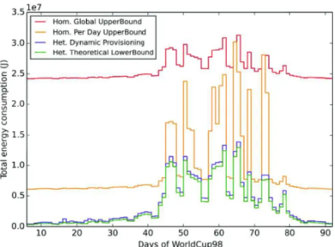
orig-Fig. 6. Total energy consumption comparison with lower and upper bounds for all days. Original traces.
TABLE II
TOTAL ENERGY DIFFERENCE PERCENTAGE OF OUR ALGORITHM
COMPARED TO LOWER AND UPPER BOUND(PER DAY) - ORIGINAL.
Energy Diff. Comp. to Lower bound Comp. to Upper Bound Best per day +5.65 % (day 46) -92.95 % (day 8) Worst per day +97.17 % (day 23) -13.19 % (day 54) Average per day +21.92 % -66.34 %
Total traces +11.72 % -60.65 %
inal traces) because during all the quite stable phase from approximately 0 to 55000 seconds, Big machines are mostly used. This architecture has a large utilization range and can consequently absorb the slight load fluctuations without many reconfigurations. Despite the fact that more Little machines are used at large scale (63 at maximum compared to 41 for original traces, which is far from the recommended number for ideal combinations), the large scale situation still has a lower Joules per Request result: 0.16 compared to 0.19 (computed as total energy consumed divided by total number of processed requests).
C. Comparative Results with Lower and Upper Bounds We compare our dynamic provisioning algorithm against a theoretical heterogeneous lower bound and two homogeneous upper bounds corresponding to existing data centre manage-ment. The considered scenarios are as follows:
• Homogeneous Global UpperBound: a data center with
a constant number of homogeneous servers during the whole execution, computed according to the peak request rate: 4089 requests/s during day 73 (40890 for traces x10). The infrastructure contains 4 (31 for traces x10)
Bigmachines that are always on. This upper bound is an
example of a classical over-provisioned data center.
• Homogeneous PerDay UpperBound: a homogeneous data
center, dimensioned each day according to the daily peak rate. This is an example of coarse grain provisioning.
• Heterogeneous Dynamic Provisioning: our chosen
in-frastructure and our dynamic provisioning algorithm
de-Fig. 7. Energy proportionality comparison with lower and upper bounds for all days. Original traces.
scribed in this paper. The total energy consumption per day contains the energy consumed by computation and by reconfigurations.
• Heterogeneous Theoretical LowerBound: the minimum
computing energy achieved with our chosen infrastructure if the data center is dimensioned every second with the ideal energy-efficient combination of machines. This is an unreachable lower bound considering no on/off latency and no on/off energy costs. This lower bound pictures also the maximum energy proportionality we could reach with our infrastructure.
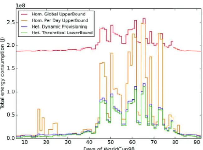
Figures 6 and 8 summarizes the results for all 86 days of the World Cup traces [15], respectively for original traces and for traces x10. Tables II and III gather the minimum, maximum and average difference percentages comparing the total energy consumption of our algorithm with the lower bound and the per day upper bound (considering the results day by day). The last line of each table is the comparison of the energy consumed during the whole World Cup traces.
Our dynamic provisioning algorithm is close to the theoreti-cal lower bound: minimum differences are +5.65% for original traces and +0.64% for large scale traces; while considering the entire execution, it consumes less than 12% more for both cases. The main difference between the results for original scale and for large scale traces concerns the comparison to the per day upper bound: for the original traces, our algorithm always consumes less than the homogeneous per day provisioning (best difference is 93%, worst is 13% and -60% for entire execution); whereas for traces x10, our dynamic provisioning algorithm consumes sometimes more than the per day provisioning (worst difference is +4%), which is mainly due to instability of the load during those days and the consequent high quantity of reconfigurations. However, considering the entire execution it achieves to consume -46% less than the homogeneous daily provisioning.
Figures 6 and 8 demonstrate the high static costs coming from classical over-provisioned data center as Homogeneous Global UpperBound, and show the advantage of our solution
Fig. 8. Total energy consumption comparison with lower and upper bounds for all days. Traces x10.
TABLE III
TOTAL ENERGY DIFFERENCE PERCENTAGE OF OUR ALGORITHM
COMPARED TO LOWER AND UPPER BOUND(PER DAY) - TRACES X10.
Energy Diff. Comp. to Lower bound Comp. to Upper Bound Best per day +0.64 % (day 81) -84.12 % (day 17) Worst per day +123.81 % (day 23) +4.49 % (day 84) Average per day +33.50 % -27.31 %
Total traces +11.91 % -46.29 %
which makes the energy consumption more proportional to the actual daily load, as also clearly shown by Figures 7 and 9. Each of these graphs is a scatter plot of the daily total energy consumption of the infrastructure regarding the daily cumulated number of requests. Therefore it can be interpreted as the energy proportionality evaluation of our heterogeneous dynamic provisioning algorithm compared to the previously described upper and lower bounds. The static costs of upper bounds are again observable, as well as the proximity of our solution with the lower bound.
VI. CONCLUSIONS ANDPERSPECTIVES
We proposed a dynamic provisioning algorithm dedicated to heterogeneous infrastructures as it takes into account the different reconfiguration temporalities of the architectures. It performs both load-reactive and energy-saving actions and suc-ceed to provision machines in time to process incoming work-load as well as to reconfigure the infrastructure towards a more energy-efficient combination when needed. We demonstrated the benefits of our original approach compared to classical data center management in terms of energy consumption and showed that it achieves energy proportionality by drastically reducing static costs. We detailed the temporal evolution of our reconfigurations over time and we also validated their efficiency for a large scale infrastructure.
As future work we will investigate the impact of load prediction errors on reconfiguration decisions, and adapt our algorithm to be able to keep a maximum quality of service despite the prediction errors. This work only focuses on energy
Fig. 9. Energy proportionality comparison with lower and upper bounds for all days. Traces x10.
proportionality of the servers, and it would be interesing to study the impacts on the cooling systems in the future.
ACKNOWLEDGMENTS
This research is partially supported by the French ANR MOEBUS project and the European CHIST-ERA STAR project. Experiments were carried out using the Grid5000 testbed, supported by a scientific interest group hosted by Inria and including CNRS, RENATER and several Universities as well as other organisations (https://www.grid5000.fr).
REFERENCES
[1] L.A. Barroso and U. Holzle. The Case for Energy-Proportional Com-puting. IEEE Computer, 2007.
[2] F. Ryckbosch, S. Polfliet, and L. Eeckhout. Trends in Server Energy Proportionality. Computer, 2011.
[3] G. Da Costa. Heterogeneity: The Key to Achieve Power-Proportional Computing. IEEE International Symposium on CCGrid, 2013. [4] V. Villebonnet, G. Da Costa, L. Lefevre, J-M. Pierson, and P. Stolf. ”Big,
Medium, Little”: Reaching Energy Proportionality with Heterogeneous Computing Scheduler. Parallel Processing Letters, 25(3), 2015. [5] E. Pinheiro, R. Bianchini, E.V. Carrera, and T. Heath. Load Balancing
and Unbalancing for Power and Performance in Cluster-Based Systems.
Workshop on compilers and operating systems for low power, 2001. [6] G. Chen, W. He, J. Liu, S. Nath, L. Rigas, L. Xiao, and F. Zhao.
Energy-aware Server Provisioning and Load Dispatching for Connection-intensive Internet Services. In USENIX Symposium on Networked
Systems Design and Implementation, 2008.
[7] M. Lin, A. Wierman, L.L.H. Andrew, and E. Thereska. Dynamic Right-Sizing for Power-proportional Data Centers. In IEEE INFOCOM, 2011. [8] D. Ardagna, S. Casolari, and B. Panicucci. Flexible Distributed Capacity Allocation and Load Redirect Algorithms for Cloud Systems. In IEEE
Int. Conf. on Cloud Computing, 2011.
[9] A-C. Orgerie, L. Lefevre, and J-P. Gelas. Chasing Gaps between Bursts: Towards Energy Efficient Large Scale Experimental Grids. In Int. Conf.
on Parallel & Distributed Comp., Applications & Technologies, 2008. [10] T. Lu, M. Chen, and L.L.H. Andrew. Simple and Effective Dynamic
Provisioning for Power-Proportional Data Centers. IEEE Transactions
on Parallel and Distributed Systems, 2013.
[11] R. Bolze et al. Grid’5000: A Large Scale And Highly Reconfigurable Experimental Grid Testbed. Int. Journal of HPC Applications, 2006. [12] F. Rossigneux, L. Lefevre, J-P. Gelas, and M. Dias de Assuncao. A
Generic and Extensible Framework for Monitoring Energy Consumption of OpenStack Clouds. In IEEE SustainCom, 2014.
[13] Lighttpd Web Server. http://www.lighttpd.net/. [14] Siege Benchmark. https://www.joedog.org/siege-home/.