O
pen
A
rchive
T
OULOUSE
A
rchive
O
uverte (
OATAO
)
OATAO is an open access repository that collects the work of Toulouse researchers and
makes it freely available over the web where possible.
This is an author-deposited version published in :
http://oatao.univ-toulouse.fr/
Eprints ID : 18475
To link to this article : DOI:
10.1140/epje/i2017-11499-2
URL :
http://dx.doi.org/10.1140/epje/i2017-11499-2
To cite this version :
Renaudière de Vaux, Sébastien and Zamansky,
Rémi and Bergez, Wladimir and Tordjeman, Philippe and Haquet,
Jean-François Magnetoconvection transient dynamics by numerical
simulation. (2017) The European Physical Journal E - Soft Matter,
vol. 40 (n° 13). pp. 1-11. ISSN 1292-8941
Any correspondence concerning this service should be sent to the repository
administrator:
[email protected]
Magnetoconvection transient dynamics by numerical simulation
⋆
S´ebastien Renaudi`ere de Vaux1,2,a, R´emi Zamansky1, Wladimir Bergez1, Philippe Tordjeman1, and
Jean-Fran¸cois Haquet2
1 Institut de M´ecanique des Fluides de Toulouse (IMFT) - Universit´e de Toulouse, CNRS-INPT-UPS, Toulouse, France 2 CEA, DEN, Cadarache, SMTA/LPMA, F13108 St Paul lez Durance, France
Abstract. We investigate the transient and stationary buoyant motion of the Rayleigh-B´enard instability when the fluid layer is subjected to a vertical, steady magnetic field. For Rayleigh number, Ra, in the range 103–106, and Hartmann number, Ha, between 0 and 100, we performed three-dimensional direct
numerical simulations. To predict the growth rate and the wavelength of the initial regime observed with the numerical simulations, we developed the linear stability analysis beyond marginal stability for this problem. We analyzed the pattern of the flow from linear to nonlinear regime. We observe the evolution of steady state patterns depending on Ra/Ha2 and Ha. In addition, in the nonlinear regime, the averaged
kinetic energy is found to depend on Ra and to be independent of Ha in the studied range.
1 Introduction
The study of magnetoconvection is fundamental in astro-physics, geophysics [1] and condensed matter physics (for instance crystal growth [2]). It is also fundamental in in-dustrial applications, as heat exchanger for nuclear fusion reactors [3], nuclear safety studies [4] or induction heating and stirring [5] in metallurgy. In this study, we focus on the dynamics and pattern motion obtained by numerical sim-ulation of magnetoconvection at low magnetic Reynolds and Prandtl numbers.
When a non-magnetic electrical conducting liquid sus-tains a constant magnetic field and a temperature gradi-ent, it undergoes the action of the driving buoyancy force, which is counterbalanced by the Lorentz force and the vis-cous force. These forces are responsible of magnetohydro-dynamic (MHD) instabilities, characterized by patterns that govern heat transfer [6, 7] and stirring efficiency. The coupling between Navier-Stokes equation and the mag-netic induction equation is determined by the value of magnetic Reynolds number Rm = µ0σUL where µ0is the
electromagnetic permeability of vacuum, σ is the electri-cal conductivity of the fluid, and U and L are the charac-teristic velocity and length of the magnetoconvection. The magnetic Reynolds number is related to the hydrodynamic Reynolds number Re by Rm = ReP m, with P m = µ0σν
the magnetic Prandtl number. In many cases, P m ∼ 10−6
⋆
Supplementary material in the form of four .avi files
avail-e-mail: [email protected]
and consequently Rm is much lower than unity, the mag-netic field is weakly perturbed and the advection of the magnetic field is negligible (O(Rm)). For incompressible liquids, small height variation and under the Oberbeck-Boussinesq approximation, three other non-dimensional parameters control the flow dynamics: the Prandtl num-ber P r = ν/κ, the Hartmann numnum-ber Ha = B0L
p σ/ρν and the Rayleigh number Ra = gβ∆T L3/νκ. Here, ν is
the kinematic viscosity, κ is the thermal diffusivity, g is the acceleration of gravity, β is the thermal expansion coeffi-cient, ∆T is a characteristic temperature difference, B0is
the magnitude of the magnetic field and ρ is the reference fluid density. Ra expresses the buoyancy to viscous force ratio, and Ha2 is the Lorentz force to viscous force ratio.
Chandrasekhar [1, 8] has developped the linear sta-bility theory for Rayleigh-B´enard magnetoconvection. He found that the convection occurs for Ra > Rac, where Rac
the critical Rayleigh number. The marginal stability curve Rac = f (Ha) is defined by a zero growth rate s = 0 of
the infinitely small perturbations. He established that for a magnetic field aligned with gravity, Rac = f (Ha), for
which Rac ∼π2Ha2 for large Ha values, experimentally
validated [9, 10]. For horizontal magnetic fields, Rac is
in-dependent of Ha. We define the relative distance to the threshold ǫ = (Ra − Rac)/Rac. One notes that for strictly
positive values of ǫ, the linear stability analysis has never been carried out. Based on a nonlinear stability analysis and for small values of Ha (Ha < 5), Busse and Clever [11] showed that stable parallel rolls form for ǫ smaller than a critical value. For larger values of ǫ, the rolls destabilize by oscillatory convection. This result has been confirmed by Direct Numerical Simulation (DNS), for Ha < 12 and
ǫ < 4 [12]. Spectral simulations have also been performed to characterize chaotic structures for a large range of ǫ, up to ∼ 500 [13]. Recently Basak et al. [14, 15] showed that the energy was proportional to ǫ for small values of ǫ < 1 and Ha < 10 using DNS in a square box. We did not find numerical studies of pattern motion and of dynam-ics for intermediate values of (Ha, Ra) and 0 < ǫ < 10 (Ha ∼ 50 and Ra ∼ 105). In particular, the transition
between the linear and nonlinear dynamics seems to have never been investigated. On the other hand, systematic experiments have been developed for this range of param-eters by Yanagisawa et al. [16,17]. The pattern motion has been characterized by ultrasonic velocimetry [18] in liquid gallium with and without horizontal magnetic field. They confirmed the structure in rolls, which is destabilized into 3D structures as Ra is increased. Moreover, in the phase diagram (Ha, Ra) they identify five flow regimes for which the patterns were characterized by their wave number. At sufficiently large values of Ra and Ha, the different phases characteristic of regime dynamics are separated by iso-lines of τmag/τbuo = Ra/Ha2, where τmag = ρ/σB20 and
τbuo= κ/gβ∆T h.
In this paper, we studied by DNS the destabilization of an electrically conducting fluid, subject to a magnetic field and to a temperature gradient, both aligned with gravity. Following the results from Chandrasekhar [1, 8], we focus on the application of a vertical magnetic field to study the effects of Ha on the marginal stability. A rectangular Rayleigh-B´enard cell is considered with an aspect ratio of 10 and periodic boundary conditions perpendicular to the vertical axis. This study was performed for Ha = 0, 9, 18 and 36, and for 104 < Ra < 1.5 · 105, with 0 < ǫ < 100.
In parallel, we realized the linear stability analysis for a large range of (Ha, Ra) values and confronted the results to DNS. The pattern motion in the nonlinear dynamics regime has been identified by DNS. We found that the transition between linear and nonlinear dynamics is deter-mined at first order by the equilibrium between potential and kinetic energies.
The paper is organized as follows. We first describe the studied configuration in sect. 2. In sect. 3, we give a brief description of the computational methods. In sect. 4, we analyse and discuss the pattern motion regarding wave-length selection.
2 Problem description
In many practical situations, confinement and boundaries play a key role. This is particularly true for MHD flows (see for example [19]). Considering infinite conditions al-lows a generalization of the results. We consider an infi-nite fluid layer of a conducting fluid, confined between two rigid, horizontal plates, as sketched in fig. 1. The fluid is subject to the action of a steady, vertical mag-netic field, and to the action of gravity. The temperatures are imposed at the walls, Tb⋆ at the bottom and Tt⋆ at
the top, so that ∆T⋆ = T
b⋆−Tt⋆ > 0. If this
temper-ature difference exceeds a critical value, buoyancy force will become larger and the cavity will exhibit convection.
Fig. 1. Sketch of the configuration. The infinite horizontal walls are assumed to have an infinite thermal conductivity. The fluid is subjected to the action of gravity (buoyancy force) and of the Lorentz force.
Under the Oberbeck-Boussinesq approximation, the non-dimensional equations for the magnetoconvection are
∂u ∂t + (u · ∇)u = −∇p + △u − Ra P rT ez+ Ha 2j × B, (1) ∂T ∂t + (u · ∇)T = 1 P r△T + Γ j 2, (2) ∂B ∂t = 1 P m△B+ ∇ × (u × B). (3)
We define the nabla operator in Cartesian coordinates ∇ ≡(∂x, ∂y, ∂z) and the Laplace operator △ ≡ ∇2.
Equa-tions (1), (2), and (3), respectively, are the Navier-Stokes equation, the heat transport equation (assuming incom-pressibility), and the induction equation, deduced from the Maxwell equations and generalized Ohm’s law. In this paper, all⋆quantities are dimensional parameters. Hence,
the variables u, p, T and B represent the non-dimensional velocity, pressure, temperature and magnetic field, and j is the current density. The current density j can either be computed using Ohm’s law or with Amp`ere’s law. Addi-tionaly, conservation of mass, electric charge and Maxwell-Thomson law read
∇ · u= ∇ · j = ∇ · B = 0. (4) To non-dimensionalize the equations, we used the fol-lowing characteristic parameters t0 = h2/ν, U = ν/h,
B0 and h1. The non-dimensional temperature is defined
by T = (T⋆−T
t⋆)/∆T⋆. The current density scale is
j0 = σUB0. The fluid is confined between two plates
lo-cated at z = 0 and z = 1. The additional non-dimensional parameter Γ = j2
0/σ∆T⋆ρcp, with cp the specific heat is
characteristic of the Joule dissipation into thermal energy. It is generally negligible in steady fields and it is not com-puted in the DNS nor in the LSA. Since P r and P m are only depending on physical properties of the fluid, they will be taken to be constant through the whole study. We used P r = 0.025 and P m = 1.55 · 10−6, as were
used for liquid gallium [20]. Γ ≈ 10−13 can be neglected.
In the configuration that was used for the DNS, we had t0≃1250 s, with h = 2 cm.
As stated by Chandrasekhar [1], a vertical magnetic field modifies the critical value of the Rayleigh number
1 With U = ν/h, Rm ≡ P m. We have checked that Rm
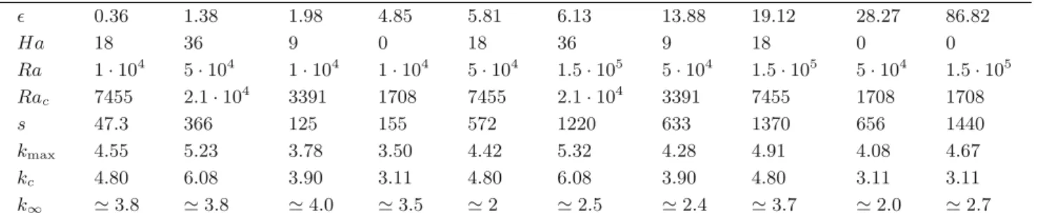
Table 1. Values of the parameters charateristics of the DNS and LSA for the ten studied cases. The critical Rayleigh Rac and
wave number kcare obtained from the marginal stability analysis; the growth rate s and the most unstable wave number kmax
are obtained by LSA; the final wave number k∞characterizes the pattern structure, and is obtained by DNS in the steady state
regime. ǫ 0.36 1.38 1.98 4.85 5.81 6.13 13.88 19.12 28.27 86.82 Ha 18 36 9 0 18 36 9 18 0 0 Ra 1 · 104 5 · 104 1 · 104 1 · 104 5 · 104 1.5 · 105 5 · 104 1.5 · 105 5 · 104 1.5 · 105 Rac 7455 2.1 · 10 4 3391 1708 7455 2.1 · 104 3391 7455 1708 1708 s 47.3 366 125 155 572 1220 633 1370 656 1440 kmax 4.55 5.23 3.78 3.50 4.42 5.32 4.28 4.91 4.08 4.67 kc 4.80 6.08 3.90 3.11 4.80 6.08 3.90 4.80 3.11 3.11 k∞ ≃3.8 ≃3.8 ≃4.0 ≃3.5 ≃2 ≃2.5 ≃2.4 ≃3.7 ≃2.0 ≃2.7
Rac beyond which convection appears. This threshold
value scales as Rac ∼ π2Ha2 in the limit of high Ha
numbers. Recall that the parameter ǫ = (Ra − Rac)/Rac
accounts for the distance to this threshold. We have inter-est in understanding the relative effects of the characteris-tic times τbuo and τmag. Therefore, we focus on the region
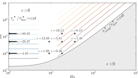
of the parameter plane (Ha, Ra) where those times re-main of relatively close importance. We restrain ourselves to the region where 0 < Ha < 100 and 0 < ǫ < 20. The computed points by DNS are given in table 1 and repre-sented in fig. 2. The blue lines represent iso-lines of τν/τbuo
and the orange lines represent the iso-lines of τmag/τbuo.
These lines can equivalently be understood as iso-lines of Ra and Ra/Ha2. One can note that the 2 points ǫ = 0.36
and ǫ = 1.38, the 3 points ǫ = 1.98, ǫ = 5.81 and ǫ = 6.13, and the 2 points ǫ = 13.88 and ǫ = 19.12, approximately have the same ratio τmag/τbuo= 35, 130 and 500,
respec-tively. The analysis of the results for these 7 points will allow to understand the effect of Ra/Ha2, of Ha at the
same Ra, and finally of Ra at the same Ha.
3 Numerical methods
Two complementary methods are used to solve the case. We performed 3D DNS of the Rayleigh-B´enard instability with a vertical constant magnetic field and the correspond-ing Linear Stability Analysis (LSA). We first introduce the DNS code Jadim, that allows complete numerical resolu-tion of the flow. We then present the LSA, which will give us the most unstable wave number kmax and the
corre-sponding eigenfrequency s. The linear stability should ac-curately account for the transient growth of the stability. 3.1 Direct numerical simulations with Jadim
We solve this case using the finite volume code Jadim, in a bi-periodic square box in x and y directions of side 10. The mesh is chosen in order to respect the DNS criteria of Gr¨otzbach [21]. The grid is composed of Nx×Ny×Nz=
256 × 256 × 64 points. The finite volume code Jadim has been already used in several different configurations. It uses a third order Runge-Kutta scheme for temporal in-tegration. The spatial derivatives are calculated with sec-ond order accuracy. Incompressibility is achieved through
a projection method. The viscous terms are calculated us-ing a semi-implicit Crank-Nicolson scheme. The descrip-tion of the numerical methods used in the computadescrip-tions can be found in Magnaudet et al. [22].
As long as the hypothesis of small magnetic Reynolds number is assumed, the magnetic field perturbation is O(Rm) compared to the other fields, and induction can be neglected. In this case, Faraday’s law reduces to ∇×E = 0, with E the electric field, and it allows to write the elec-tric field as the gradient of a potential Φ. This is the so-called quasi-static approximation. Therefore, Ohm’s law reduces to:
j= −∇Φ + u × ez. (5)
Electric charge conservation ∇ · j = 0 is ensured by a Poisson equation on the electric potential Φ:
△Φ = ∇ · (u × ez). (6)
This method is used in the DNS to compute the Lorentz force. Equation (6) is solved using the PETSc library [23]. A first order scheme was used to compute the gradient of Φ. As boundary conditions for the velocity, we sider a no-slip condition. We assume infinite thermal con-ductivity of the walls. This translates into a Dirichlet’s condition for the temperature at the walls. In the same way we assume walls as perfect electrical conductors. In terms of electric potential, this amounts to saying that the electric potential Φ is imposed at the walls. Without loss of generality, we can assume that Φ = 0. Physically, this corresponds to enclosing the liquid between highly thermally and electrically conducting, and non-magnetic plates (such as copper, see for example [16]). As Joule dis-sipation is not significant for steady fields and relatively low Ha numbers, this source term is not computed in the DNS. For t < 0, the fluid is at rest at uniform temperature; at t > 0 the temperature of the bottom is set to 1. The non-dimensional fluid velocity field is initiated with ran-dom values of magnitude 10−15. We compared the
numer-ical results obtained for 64 × 256 × 256 and 128 × 512 × 512 mesh grids at Ha = 36, Ra = 1.5 · 105 to verify the
nu-merical convergence. This case has been chosen because it corresponds to the thinnest Hartmann layer in our study. From this comparison we estimate that the velocity profile is calculated with an error of 4%.
Fig. 2. DNS points displayed in the parameter space (Ha, Ra). The arrows show the three cases at Ha = 0. The marginal stability curve is defined by ǫ = 0. All points located above this curve (ǫ > 0, white region) are unstable and will exhibit convection. Iso-lines of τvis/τbuoare drawn in blue by and iso-lines of τmag/τbuoare drawn in orange.
3.2 Linear stability analysis
We follow here Chandrasekhar in establishing the alge-braic linear system for the amplitudes of the perturbed fields. The equilibrium solution of the system (3) is given by (u, T, B) = (0, 1 − z, 1ez), and this solution is used
as the base state at t = 0. We linearly perturb this base state. We call the vertical velocity perturbation w, the temperature perturbation ϑ, and the vertical magnetic field perturbation bz. Here, the current density is given by
Maxwell-Amp`ere’s law, j = 1
P m∇×b. Taking −∇×∇×(1)
ensures the elimination of the gradient terms and of the complex terms. We then linearize (2) and the components along the z-axis of −∇ × ∇ × (1) and (3). Finally we have the set of equations (7) to (9)
∂△w ∂t = △ 2w +Ra P r µ ∂2ϑ ∂x2 + ∂2ϑ ∂y2 ¶ +Ha 2 P m ∂△bz ∂z , (7) ∂ϑ ∂t = 1 P r△ϑ + w, (8) ∂bz ∂t = 1 P m△bz+ ∂w ∂z . (9)
Note that the Joule dissipation term does not appear any more, since it is a second order term. However, this ap-proach, compared to DNS, takes into account the time-dependent perturbation of the magnetic field. The LSA results have confirmed that it is negigible. Considering disturbances as two-dimensional waves in the horizontal plane of assigned wave numbers kx and ky in x- and
y-directions gives w ϑ bz = W (z) Θ(z) B(z) | {z } X(z) exp(i(kxx + kyy) + st). (10)
Here, W (z), Θ(z) and B(z) are the initial amplitudes of the disturbances, and s is growth rate of the disturbance.
Using the form given by eq. (10) in system (7), it is pos-sible to write the equations in the form of an eigenvalue problem sL1X(z) = L2X(z), (11) where: L1= (D2−k2) 0 0 0 1 0 0 0 1 , (12) L2= (D2−k2)2 −Ra P rk 2 Ha2 P m[D(D 2−k2)] 1 1 P r(D 2−k2) 0 D 0 1 P m(D 2−k2) , (13) with D ≡ dzd and k2 = k2
x+ k2y. Each block L2,mn
rep-resents the action of the n-th variable on the m-th vari-able. This system is solved with finite differences using second order schemes. The details of calculation are given in appendix A. Following the same boundary conditions as for the DNS, we consider infinitely thermally and elec-trically conducting walls. If the external media is a perfect electrical conductor, the time-dependant perturbation of the magnetic field inside it is instantly relaxed. Therefore we can assume a homogeneous Dirichlet’s condition for the perturbation of the magnetic field. The same condi-tion goes for the temperature perturbacondi-tion. The bound-ary conditions, following the no-slip condition, the con-tinuity equation, and the perfectly conducting walls, are then
W = DW = Θ = B = 0 (14)
for z = 0, 1. Solving the system (11) gives the growth rate (or eigenfrequency) s of the system and the most
un-Fig. 3.Comparison of vertical velocity profiles obtained with DNS (solid line) and LSA (dots) in the linear regime. Both curves are normalized by their value at z = 1/2.
stable wave number kmax, that corresponds to an
eigen-vector X(z) = (W (z), Θ(z), B(z)). The case s = 0 was solved by Chandrasekhar [1] and gives the values of Rac
as a function of Ha. It corresponds to the solution of ǫ = 0, represented by the boundary between the white and grey regions in fig. 2. We observe a very good agree-ment between the LSA results and Chandrasekhar’s pre-dictions. We have extended this analysis to overcritical values Ra > Rac, in order to assess the transient growth
of the instability. We have checked that the difference in s between grids of size 256 and 512 was less than 1%.
4 Results and discussion
4.1 Short and large timescales behavior
In the DNS, the system is initiated with a uniform cold temperature T = 0, and the fluid is at rest, with a small random noise. The temperature at the bottom wall is im-posed at T = 1. The high thermal conductivity of the fluid (i.e. low P r) allows the establishment of a linear conducting profile in a few time steps. From then, buoy-ant motion starts to rise in the quiescent liquid. During those first instants, a profile of vertical velocity matches the profile given by linear stability (i.e. eigenvector). This is found to be valid for any profile taken at any random co-ordinates (x, y). Figure 3 shows one profile obtained with Jadim, compared with the linear stability, both normal-ized by their value at z = 1/2. The agreement between the two approaches is valid until the end of the linear regime. Here we define the linear regime by the validity of the LSA that corresponds to the instability growth.
Next, we consider the quantity w⋆2(z⋆= h/2) = 1
S Z Z
S
w⋆2(z⋆= h/2)dx⋆dy⋆, (15)
with w⋆ the velocity in SI units and S the surface of the
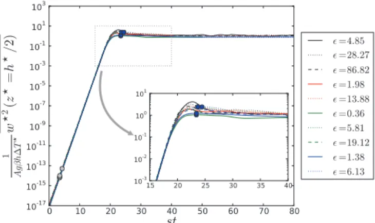
wall. This quantity represents the contribution of the ver-tical component of velocity to kinetic energy, averaged in the mid-plane. The evolution of this quantity is shown in fig. 4 for both DNS and LSA. Here, w⋆ is scaled by the
characteristic buoyant velocity. We observe a phase where the velocity grows as exp(st), where s is the LSA growth rate of the instability. Its value depends both on Ra and Ha, which will be later discussed. All the curves collapse
Fig. 4. Dynamic behavior by DNS and LSA for all the com-puted points. We used the average value of the factor A to normalize the curves. Inset: zoom on the transition between the linear and nonlinear regime.
into one master curve during the exponential growth of the instability, when plotted as a function of st. After this exponential growth, nonlinear effects become significant and the flow is reorganized until the stationary stage is reached.
The simulations show that for ǫ = 1.38 and ǫ = 5.81 which correspond to the same Ra and different Ha, the final values of w2(z = 1/2) are identical. Moreover, the
plateau value in the nonlinear regime is a function of Ra. Based on this results, it is possible to estimate the final value of w⋆2(z⋆= h/2) by a simple energy balance
be-tween kinetic energy and potential energy. This condition reads
w⋆2(z⋆= h/2) = A gβh∆T⋆, (16)
where A is a factor to be determined. This relation is equivalent to W2∼Ra. We stress that this estimate does
not take into account the Lorentz and viscous forces. Con-sequently, the DNS results show that all the curves can be superimposed in the linear and nonlinear regimes, as seen in fig. 4. The value of A using the DNS results is found to be A = 0.10 ± 0.02 for all the simulations.
Around the transition between the linear and nonlinear regimes (st ≈ 20 for our initial conditions), we do not observe an exact overlap. The simulations display that Ha contributes significantly to the amplitude of the yield kinetic energy. In conclusion, the linear regime is governed by (Ra, Ha), and the nonlinear regime by Ra.
In fig. 4, the timescale was obtained from s given by LSA (eq. (11) and table 1). Based on LSA, a systematic computation of s has been realised for 103≤Ra ≤ 1.5·105
and 0 ≤ Ha ≤ 100 (fig. 5). We observe that s is a decreas-ing function of Ha at constant Ra (dampdecreas-ing effect of mag-netic field), and an increasing function of Ra at constant Ha. Moreover ǫ is not a self-similarity parameter and s is not an univoque function of ǫ. For any value of (Ha, Ra) in the variation range studied by LSA, it is now possible to determine the s value from fig. 5 which fixes the scaling in the linear regime. Our computed points in DNS appear in red circles in this figure.
Fig. 5.Growth rate s vs. Ra for 0 ≤ Ha ≤ 100. The step of 5 in Ha is fixed for two adjacent isolines. The points computed with DNS are represented by the red circles.
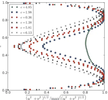
Fig. 6.Time and space averaged profiles of tangential velocity in the steady state nonlinear regime, for the DNS referenced in table 1. The curves are normalized to their maximum value and the bar denotes averaging in (x, y)-directions.
In fig. 6, we show profiles of time and space averaged velocity tangential to the Hartmann walls (orthogonal to the magnetic field) for several points. Without magnetic field (Ha = 0, Ra = 104and ǫ = 4.85), the boundary layer
thickness is of order δ ≃ 0.14 (defined as the distance to the wall corresponding to the maximum of the tangential velocity). When a magnetic field is applied, Hartmann lay-ers are likely to form and modify the velocity field. In the case Ha = 9 and Ra = 104 (ǫ = 1.98), the turbulent
mo-tion is suppressed compared to the case where Ha = 0 and the boundary layer is thicker, δ ≃ 0.19. Further increase of Ha shows a thinning of the boundary layer thickness due to the magnetic field effects. Thus, from Ha = 9, we find that δ decreases with Ha accordingly to a general trend in the Hartmann problem, coupled with thermal effects.
It is also noticeable that the points ǫ = 0.36 and ǫ = 5.81 at the same Ha = 18 have a same boundary layer thick-ness: δ ≃ 0.14 ± 0.01. A same boundary layer thickness is also measured for the points ǫ = 1.38 and ǫ = 6.13 (Ha = 36): δ ≃ 0.09 ± 0.01.
4.2 Patterns motion
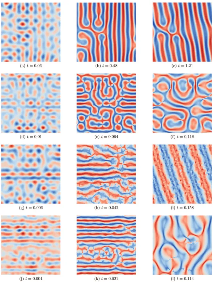
In this section we discuss four characteristic cases which are physically representative (ǫ = 0.36, 1.38, 5.81 and 6.13). DNS allows to determine the motion structures and their evolutions in time for the four values of ǫ. The spatial distribution of vertical velocity at z = 1/2 was analyzed by Fourier transform and the velocity structures were char-acterized by their wave vectors. In Supplementary Ma-terial, motion pictures of the patterns are presented in regard of the time evolutions of the kinetic energy, its spectral density, and the 2D wave vector distribution in the plane orthogonal to the magnetic field and the gravity (see videos). The movies show that the structures in linear and nonlinear regimes (st < 20 and st > 20, respectively) are strongly different. Figure 7, extracted from movies, presents three snapshots of W in the mid-plane, normal-ized by the instantaneous amplitude for the four ǫ value.
Each row corresponds to one DNS and each column to a snapshot in the linear regime, at the peak value of the kinetic energy in the mid-plane, and in the nonlinear steady state. They respectively correspond to the blue, grey and white circles in fig. 4.
In the linear part of the fig. 4, the structures develop into periodic and isotropic cells independent of time (first column of fig. 7). The spectral analysis of the patterns shows that the wave number kmax in DNS is very well
predicted by LSA in the early phase. For the four simu-lated cases, kmaxis lower but close to critical wave number
at the marginal stability kc. These results can be seen in
fig. 8 which shows, as an example, the energy spectral den-sity at different times for ǫ = 0.36. The peak at t = 0.06 perfectly matches the kmaxprediction of LSA. This result
is valid for all the computed points in table 1. The LSA at supercritical values of ǫ improves the prediction of the lin-ear behavior compared to the classic marginal theory [1]. In fig. 8 we found that kmax < kc in the linear phase.
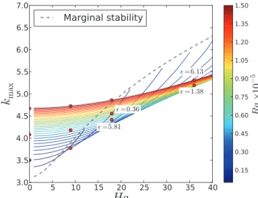
However this result cannot be generalized for a large range of (Ha, Ra). Figure 9 compares the variations of kmax
and kc for 0 ≤ Ha ≤ 40 and 104 ≤ Ra ≤ 1.5 105,
obtained by LSA. First we note that kc increases
dras-tically with Ha. Secondly, for Ha . 10, kmax increases
with Ra. However, for higher Ha values, kmax decreases,
then increases again with Ra. This means that kmax can
be smaller or larger than kc, depending on Ha and Ra.
Thirdly, for all values Ha, kmax seems to reach a plateau
value when Ra increases. This plateau value is larger than kcat low Ha and smaller than kcat high Ha. This
asymp-totic value is weakly dependent on Ha. Hence the ef-fect of the magnetic field does not seem to play a sig-nificant role at values of Ra much larger than Rac. On
the other hand, close to Rac, as for the marginal stability
Fig. 7. Snaphots of normalized vertical velocity for different times at z = 1/2 for ǫ = 0.36 (panels (a) to (c)), ǫ = 1.38 (panels (d) to (f)), ǫ = 5.81 (panels (g) to (i)), and ǫ = 6.13 (panels (j) to (l)), by DNS (red is positive and blue is negative). The first column corresponds to a snapshot during the linear regime, the second one is taken during the transition between the linear and nonlinear regime (the times are indicated in fig. 4), and the third one is characteristic of the steady state nonlinear regime. The snapshots are extracted from the DNS movies.
Fig. 8.Energy spectral density for ǫ = 0.36 in the linear regime (t = 0.06), at the maximum of the kinetic energy (t = 0.48) and in the steady state nonlinear regime (t = 1.21). The wave number values at the marginal stability kc and calculated by
the LSA kmax are given for comparison.
Fig. 9.Wave number kmax vs.Ha. Each colored curve
corre-sponds to a constant Ra.
This can be explained by considering that the character-istic width of the rolls is determined by the product of the characteristic time of cooling and the velocity close to the upper wall. This velocity decreases with Ha due to the Lorentz force.
After linear growth, a transition phase takes place, where nonlinear effects come into play, before reaching the stationary state. The structures evolve continuously and we found that this evolution is not characterized by a first order transition. For the four ǫ values, the wave number characteristic of the velocity structure is closed to kmaxat the maximum kinetic energy (fig. 8). At this peak,
nonlinear effects become dominant and the wave number decreases towards a steady value that we name k∞.
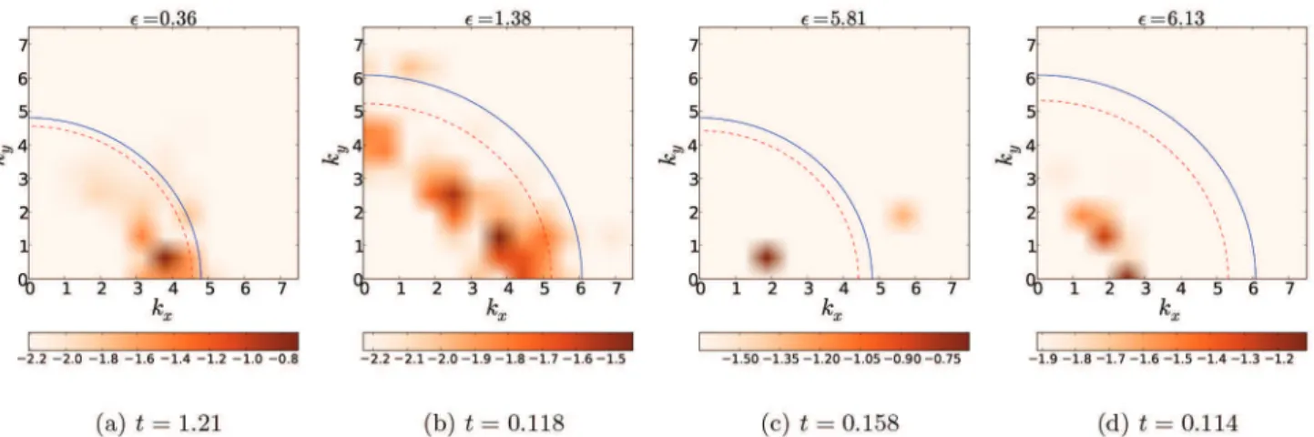
The steady state velocity patterns in nonlinear regime are presented in the right column of fig. 7, and all the structures are characterized by their 2D wave vector dis-tribution in fig. 10. The blue circle corresponds to kc
pre-dicted by Chandrasekhar [1] and the red dashed circle is kmax predicted by LSA. During the linear phase, the
en-ergy is concentrated on the circle of radius kmax(see videos
in Supplementary Material and the curve for t = 0.06 in fig. 8). In the case ǫ = 0.36 the small cells of the linear regime merge into slightly larger rolls (fig. 7(b)) which persist in time. In the steady state the velocity structure is frozen-like. In fig. 10(a), we see that most of the energy is localized in one direction associated to a lamellar structure. The wave number decreases down to an asymptotic value k∞ ≃ 3.7, which remains close to
kmax= 4.55.
In the case ǫ = 1.38, the cells merge and form larger roll-like structures. These tortuous structures remain sta-ble and evolve very slowly. The norm of the wave vector is lower than kmax, around a value k∞ ≃ 4.0. The main
difference in comparison with the case ǫ = 0.36 is that the energy tends to be istropically distributed. These tortuous structures seem to be related to spiral defect chaos (SDC) observed by Morris et al. [24].
In case ǫ = 5.81, at the peak of transition (fig. 7(h)), the cells tend to reorganize in tortuous rolls, but this structure is only transient. It then degenerates in large cells around k ≃ 2.5 before further reorganizing in par-allel rolls in the stationary regime with a wave number k∞ ≃ 2.0 (fig. 7(i)). These rolls display an oscillation
which seems to be linked to a secondary instability [11]. In this case, the energy in Fourier space is mainly localised in a unique direction as seen in fig. 10(c). The secondary peak at k = 6.0 is characteristic of the smaller structures of the rolls. In this case the dominant wave number in the stationary regime departs significantly from LSA.
The behavior of the flow for ǫ = 6.13 during the tran-sition is similar to the one for ǫ = 5.81. At the beginning of the transition, the cells merge in rolls (as seen in the DNS movies). Subsequently, these rolls transform in cell patterns, which persist contrary to the previous case. This steady state is similar to the case ǫ = 1.38 but with a dif-ferent final wave number k∞ ≃ 2.5. The energy density
spreads towards smaller wavelength (see Supplementary videos).
The analysis of these four typical cases (ǫ = 0.36, 1.38, 5.81 and 6.13) shows that the results seem to be coherent. The two cases ǫ = 0.36 and ǫ = 1.38 correspond to the same Ra/Ha2 ≈ 35. On the other hand, ǫ = 5.81 and
ǫ = 6.13 correspond to Ra/Ha2 ≈ 130. For isolines of
Ra/Ha2close to the marginal stability curve, the patterns
in the steady state nonlinear regime are characterized by a wave number lower but close to kmax(obtained from LSA).
For larger values of Ra/Ha2, the characteristic sizes of the
structures are larger and k∞ is smaller than kmax. In this
case the transition dynamics leading to the steady state nonlinear regime is more complex and shows permanent reorganization due to higher Ra.
Fig. 10. 2D normalized energy spectra of the vertical velocity W (z = 1/2), for ǫ = 0.36 ǫ = 1.38, ǫ = 5.81, and ǫ = 6.13 in the steady state nonlinear regime. The data are normalized by the total energy. The colors are in log-scale. These spectra correspond to the snapshots of the third column in fig. 7. The marginal wave number kc (solid blue circle) and kmax (dashed
red circle) calculated by LSA are given for comparison.
Considering all the studied cases, the DNS seems to display a structural transition between lamellar and tor-tuous when Ha increases and ǫ < 10. Indeed, at Ha = 9 and 18 (ǫ = 1.98, ǫ = 0.36 and ǫ = 5.81), the patterns are lamellar; at Ha = 36 (ǫ = 1.38 and ǫ = 6.13), the patterns are tortuous lamellar. This tortuous structure could be understood as a coupling effect of buoyancy force and Lorentz force acting of the velocity field in the three directions. The joint effect of these two forces is to cre-ate a torque which bends the lamellar structures if Ha is high enough. For ǫ > 10 (ǫ = 13.88 and ǫ = 19.12), the structures become similar to thermoconvection without magnetic effect. These two cases are far enough from the marginal stability curve and the buoyancy force becomes dominant.
5 Concluding remarks
In this paper, we studied the transient dynamics of a liquid metal in magnetoconvection. We computed the velocity patterns by DNS for various value of ǫ = (Ra − Rac)/Rac
corresponding to intermediate (Ha, Ra) values. The char-acteristic lengths of the patterns were measured during the transient dynamics: linear regime, nonlinear transi-tion and steady regime. We have developed a LSA code, in order to determine the growth rate and the wave num-ber of the instability. We observe a very good agreement between the DNS results in the linear regime and the LSA predictions. From the DNS, the wave vectors characteris-tic of the structures appear to be isotropic and the maxi-mum of the energy density matches the value kmaxof the
LSA. It is to note that the methods for computing the Lorentz force differ in the two approaches. In the DNS we used the quasi-static model and in the LSA we solved for the perturbation of B. Both methods should agree in the P m = 0 limit. Here these approaches are consistent, ow-ing to the smallness of P m. We found that the dynamics is
self-similar except around the transition between the two regimes where the total energy of the system yields a max-imum. The time scaling in the linear regime is based on the growth rate, and in the steady state nonlinear regime, the energy scaling is given by Ra and is independent of Ha at first order.
In the steady state nonlinear regime the patterns present large differences with Ra and Ha. For cases neigh-bouring the marginal stability (ǫ = 0) and with a same Ra/Ha2 ratio, the wave number k
∞ is lower, but very
close to kmax. For cases far away from the marginal
stabil-ity and at constant Ra/Ha2, the wave number k
∞< kmax.
Therefore, an increase in Ra/Ha2generates a decrease in
k∞. Furthermore, the structure types are determined by
Ha in the steady state nonlinear regime. For Ha = 9 and 18, we observe a lamellar structure. Increasing to Ha = 36 shows that there is a structural transition: the rolls be-come tortuous. This study will be extended to a large range of ǫ values and to frequency effects when AC mag-netic fields are applied.
The authors greatly acknowledge the help of Anna¨ıg Pedrono for the numerical developments in the Jadim code. This work was granted access to the HPC resources of CALMIP super-computing center. Financial support from the french Nuclear Energy Center (CEA) in Cadarache and from the ECM com-pany in Grenoble are acknowledged.
Appendix A. Finite differences schemes for
stability analysis
We give in this appendix the numerical schemes that were used for the linear stability analysis. The operators in equations (12) and (13) can be expressed with finite dif-ferences, in order to solve the linear system (11).
Appendix A.1. Numerical schemes
Let us consider the vector x that either stands for W , Θ, or B and we discretize in the z-direction and for a number of points Nz, the space step is ∆z = N1
z. We
choose the following second order schemes to approximate the derivatives: x′i = xi+1−xi−1 2∆z , (A.1) x′′i = xi+1+ xi−1−2xi ∆z2 , (A.2) x′′′i =
xi+2−xi−2−2xi+1+ 2xi−1
2∆z3 , (A.3)
x(4)i =
xi+2+ xi−2−4xi+1−4xi−1+ 6xi
∆z4 . (A.4)
Let us express X and the operators L1 and L2 from
eq. (11) with finite differences
X= (W1, · · · , WNz, Θ1, · · · , ΘNz, B1, · · · , BNz) T , (A.5) Lk = Lk,11 Lk,12Lk,13 Lk,21 Lk,22Lk,23 Lk,31 Lk,32Lk,33 , (A.6)
with k = 1 or 2. Each matrix Lk,ij is a Nz×Nz matrix.
As shown in the following paragraph, the matrices L1and
L2 depend on Ra, Ha, P r, P m and k.
Appendix A.2. Expression of the matrices
We can note that the matrices L1,ijand L2,ijwill be (n +
1)-diagonal where n is the order of derivation. Replacing the terms in eqs. (1), (2) and (3) with the expressions given by eqs. (A.1) to (A.4) reads
L1,11 = 1 ∆z2 a11 11a1211 0 · · · 0 1 −2 1 . .. ... 0 . .. ... . .. 0 .. . . .. 1 −2 1 0 · · · 0 aNz,Nz−1 11 a Nz,Nz 11 , (A.7) L1,22 = I, (A.8) L1,33 = I, (A.9) L1,ij,i6=j = 0, (A.10)
where I is the identity matrix. The terms a11 11, a1211,
aNz,Nz−1
11 and a
Nz,Nz
11 will be given by the boundary
condi-tions. Those matrices represent the terms on the left side of the equations, and except for L1,11, there is no
deriva-tive term which implies the matrices to be diagonal. The L2,ij matrices represent the coupling between the
differ-ent equations. Let b(0)ij , b (−1) ij , b (−2) ij , b (+1) ij , b (+2) ij be the
main, first lower, second lower, first upper and second up-per diagonal terms of the matrix. The inner aspect of the matrix is L2,ij= . .. ... ... ... ... b(−2)ij b (−1) ij b (0) ij b (+1) ij b (+2) ij . .. ... ... ... ... . (A.11)
The other terms are all equal to zero. The two first and the two last lines will be given by the boundary conditions. We can first express the L2,11, L2,22, L2,33 matrices. The
L2,11 matrix is pentadiagonal and we have
b(0)11 = 6 ∆z4 + 4 k2 ∆z2 + k 4, (A.12) b(+1)11 = b(−1)11 = − 4 ∆z4 − 2k2 ∆z2, (A.13) b(+2)11 = b(−2)11 = 1 ∆z4. (A.14)
The L2,22 et L2,33 matrices are tridiagonal, hence b(+2)22 =
b(−2)22 = b(+2)33 = b(−2)33 = 0. We can express the other terms as b(0)22 = − 1 P r k2+ 2 ∆z2 , (A.15) b(+1)22 = b(+1)22 = 1 P r 1 ∆z2, (A.16) b(0)33 = − 1 P m k2+ 2 ∆z2 , (A.17) b(+1)33 = b (+1) 33 = 1 P m 1 ∆z2. (A.18)
The L2,13and L2,31are also pentadiagonal and tridiagonal
matrices and the diagonal terms can be expressed as
b(0)13 = 0, (A.19) b(+1)13 = −b (−1) 13 = Ha2 P m µ 1 ∆z3 + k2 2∆z ¶ , (A.20) b(+2)13 = b (−2) 13 = 1 2∆z3, (A.21) b(0)31 = 0, (A.22) b(+1)31 = −b (−1) 31 = 1 2∆z. (A.23)
Since the magnetic field and the temperature do not influence each other, the L2,23 and L2,32 are empty. If
we took in consideration the Joule dissipation, the L2,32
would not be zero, but since the equations were linearised and the Joule dissipation is a second order term, it does not appear here. L2,12and L2,21are diagonal matrices and
are expressed as L2,12= − Ra P rk 2 I, L2,21 = I. (A.24)
References
1. S. Chandrasekhar, Hydrodynamic and Hydromagnetic Sta-bility (Clarendon Press, 1961).
2. R. Moreau, Prog. Crystal Growth 38, 161 (1999). 3. H. Branover, Metallurgical Technologies, Energy
Conver-sion, and Magnetohydrodynamic Flows, Vol. 148 (AIAA, 1993).
4. Ch. Journeau, P. Piluso, J.F. Haquet, S. Saretta, E. Boc-caccio, J.M. Bonnet, Proc. ICAPP (2007).
5. E. Taberlet, Y. Fautrelle, J. Fluid Mech. 159, 409 (1985). 6. J.M. Aurnou, P.L. Olson, J. Fluid Mech. 430, 283 (2001). 7. U. Burr, U. M¨uller, Phys. Fluids 13, 3247 (2001). 8. N.O. Weiss, M.R.E. Proctor, Magnetoconvection
(Cam-bridge University Press, 2014). 9. Y. Nakagawa, Nature 175, 417 (1955).
10. Y. Nakagawa, Proc. R. Soc. London, Ser. A 240, 108 (1957).
11. F.H. Busse, R.M. Clever, Phys. Fluids 25, 931 (1982). 12. Y. Nandukumar, P. Pal, EPL 112, 24003 (2015).
13. W.M. Macek, M. Strumik, Phys. Rev. Lett. 112, 074502 (2014).
14. A. Basak, R. Raveendran, K. Kumar, Phys. Rev. E 90, 033002 (2014).
15. A. Basak, K. Kumar, Eur. Phys. J. B 88, 1 (2015). 16. T. Yanagisawa, Y. Yamagishi, Y. Hamano, Y. Tasaka, M.
Yoshida, K. Yano, Y. Takeda, Phys. Rev. E 82, 016320 (2010).
17. T. Yanagisawa, Y. Hamano, T. Miyagoshi, Y. Yamagishi, Y. Tasaka, Y. Takeda, Phys. Rev. E 88, 063020 (2013). 18. Y. Takeda, Ultrasonic Doppler Velocity Profiler for Fluid
Flow, Vol. 101 (Springer Science & Business Media, 2012). 19. R. Moreau, Magnetohydrodynamics (Springer Science &
Business Media, 1990).
20. M.J. Assael, I.J. Armyra, J. Brillo, S.V. Stankus, J. Wu, W.A. Wakeham, J. Phys. Chem. Ref. Data 41, 033101 (2012).
21. G. Gr¨otzbach, J. Comput. Phys. 49, 241 (1983).
22. J. Magnaudet, M. Rivero, J. Fabre, J. Fluid Mech. 284, 97 (1995).
23. S. Balay, S. Abhyankar, M.F. Adams, J. Brown, P. Brune, K. Buschelman, L. Dalcin, V. Eijkhout, W.D. Gropp, D. Kaushik, M.G. Knepley, L.C. McInnes, K. Rupp, B.F. Smith, S. Zampini, H. Zhang, PETSc users manual, Tech-nical Report ANL-95/11 - Revision 3.6 (Argonne National Laboratory, 2015).
24. S.W. Morris, E. Bodenschatz, D.S. Cannell, G. Ahlers, Phys. Rev. Lett. 71, 2026 (1993).