New developments of the Extended Quadrature Method of Moments to solve Population Balance Equations

O

pen

A

rchive

T

OULOUSE

A

rchive

O

uverte (

OATAO

)

OATAO is an open access repository that collects the work of Toulouse researchers and

makes it freely available over the web where possible.

This is an author-deposited version published in : http://oatao.univ-toulouse.fr/

Eprints ID : 22828

To link to this article :DOI:1016/j.jcp.2018.03.027

URL http://dx.doi.org/

10.1016/j.jcp.2018.03.027

To cite this version : Pigou, Maxime and Morchain, Jérôme and

Fede, Pascal and Penet , Marie-Isabelle: New developments of the

Extended Quadrature Method of Moments to solve Population Balance

Equations (2018), Journal of Computational Physics, vol. 365,

pp.243-268

Any correspondance concerning this service should be sent to the repository

administrator: staff-oatao@listes-diff.inp-toulouse.fr

New

developments

of

the

Extended

Quadrature

Method

of

Moments

to

solve

Population

Balance

Equations

Maxime Pigou

a

,

b

,

∗

_,

_{Jérôme Morchain}

a

_,

_{Pascal Fede}

b

_,

_{Marie-Isabelle Penet}

c

_,

Geoffrey Laronze

c

a_{LISBP,UniversitédeToulouse,CNRS,INRA,INSA,Toulouse,France}

b_{InstitutdeMécaniquedesFluidesdeToulouse–UniversitédeToulouse,CNRS-INPT-UPS,Toulouse,France} c_{SanofiChimie–C&BDBiochemistryVitry- 9quaiJulesGuesde,94400Vitry-sur-Seine,France}

a

b

s

t

r

a

c

t

Keywords:

ExtendedQuadratureMethodofMoments (EQMOM)

QuadratureBasedMethodofMoments (QBMM)

PopulationBalance Mathematicalmodelling Gaussquadrature

Population Balance Models have a widerange ofapplications in manyindustrial fields as theyallowaccountingforheterogeneityamongpropertieswhichare crucialforsome system modelling. They actually describe the evolution of aNumber Density Function (NDF) using a Population Balance Equation (PBE). For instance, they are applied to gas–liquid columns orstirred reactors, aerosoltechnology, crystallisationprocesses, fine particles orbiologicalsystems.Thereisasignificantinterestforfast, stableandaccurate numerical methods in order to solve for PBEs, a classof such methods actually does not solvedirectlytheNDFbutresolvestheirmoments.Thesemethodsofmoments,and in particular quadrature-based methods ofmoments, have been successfully applied to a varietyof systems.Point-wise values ofthe NDF are sometimesrequired butare not directlyaccessible fromthemoments.To addresstheseissues,the ExtendedQuadrature MethodofMoments(EQMOM)hasbeendevelopedinthepastfewyearsandapproximates the NDF, fromitsmoments,as aconvexmixtureofKernel DensityFunctions (KDFs)of the same parametric family. In the present work EQMOMis further developed ontwo aspects.Themainoneisasignificantimprovementofthecoreiterativeprocedureofthat method,thecorrespondingreductionofitscomputationalcostisestimatedtorangefrom 60%upto95%.ThesecondaspectisanextensionofEQMOMtotwonewKDFsused for theapproximation,theWeibullandtheLaplacekernels.AllMATLABsourcecodesusedfor thisarticleareprovidedwiththisarticle.

1. Introduction

PopulationBalanceEquations(PBEs)are particularformalismsthatallowsdescribingtheevolutionofpropertiesamong heterogeneous populations. Theyare used to trackthesize distribution of fineparticles [1]; thebubble size distribution ingas–liquidstirred-tankreactorsorbubblecolumns[2,3];thecrystal-sizedistributionincrystallizers; thedistributionof biologicalcellpropertiesinbioreactors[4,5];thevolumeand/orsurfacedistributionofsootparticlesinflames[6,7] orthe formationofnano-particles[8],amongotherexamples.

*

Correspondingauthorat:LISBP-INSAToulouse,135AvenuedeRangueil,31077Toulouse,France.

Nomenclature Greek symbols

ε

relativetolerance

λ

j j-thnestedquadraturenode

µ

positivemeasure

ω

j j-thnestedquadratureweight

Ä

ξ NDFsupport

π

k k orderorthogonalpolynomial

σ

shapeparameter

ξ

randomvariable

ξ

i i-thmainquadraturenode

ζ

realisabilitycriteriaon]0

_{, +∞}

[

Roman

a orthogonalpolynomialsrecurrencecoefficient

A transitionmatrixtodegeneratedmoments

b orthogonalpolynomialsrecurrencecoefficient

H

Hankeldeterminant Jn n orderJacobimatrix mk momentoforderk

M

realisablemomentspace

n numberdensityfunction

e

n approximationofn N orderofmomentset

N

orderofrealisability

pk canonicalmomentoforderk P numberofmainquadraturenodes

Q numberofnestedquadraturenodes

wi i-thmainquadratureweight

A PBE describes the evolution and transport of a Number Density Function (NDF), under the influence of multiple processeswhichmodifythetrackedpropertydistribution(e.g.erosion,dissolution,aggregation,breakage, coalescence, nu-cleation,adaptation,etc.).

One often requires low-cost numerical methods to solve PBEs, for instance when coupling with a flow solver (e.g. Computational Fluid Dynamics software). Monte-Carlo methods constitute a stochastic resolution of the popula-tion balance and can be applied to such PBE–CFD simulations [9]. Similarly, sectional methods allow direct numeri-cal resolutions of the PBE through the discretisation of the property space [10,11]. They respectively require a high number of parcels or sections in order to reach high accuracy and are thus often discarded for large-scale simula-tions.

Aninterestingalternative approachliesinthefield ofmethodsofmoments.APBE,whichdescribestheevolutionofa NDF,istransformedinasetofequationswhichdescribestheevolutionofthemomentsofthatdistribution.Momentsare integralpropertiesofNDFs,thefirstloworderintegermomentsarerelatedtothemean,variance,skewnessandflatnessof thestatisticaldistributionsdescribedbyNDFs.Thisapproachthenreducesthenumberofresolvedvariablestoafinitesetof NDFmoments.Italsocomeswithsomedifficultieswhenonemustcomputenon-momentintegralproperties,orpoint-wise evaluations,ofthedistribution[12].

Totackletheseissues,onecantrytorecoveraNDFfromafinitesetofitsmoments.Inmostcases,thisreverseproblem hasaninfinitenumberofsolutionsanddifferentapproachesexisttoidentifyoneoranotherout ofthem.Thesimplestis probablytoassume thattheNDFisastandarddistribution(Gaussian,Log-normal,. . . ) whoseparameters willbededuced fromits firstfew moments.Othermethods thatleadto continuousapproximations, andwhich preserveahighernumber ofmoments,aretheSplinemethod[13],theMaximum-Entropyapproach[12,14,15] ortheKernelDensityElementMethod (KDEM)[16].

Morerecently,theExtendedQuadratureMethodofMoments(EQMOM)wasproposedasanewapproachwhichismore stablethanthepreviousones,andyieldseithercontinuousordiscreteNDFsdependingonthemoments[1,17,18].EQMOM has been implemented in OpenFOAM [19] for the purpose of PBE–CFD coupling. The core of this method relies on an iterativeprocedurethatisacomputationalbottleneck.

The current work focuses on EQMOM and develops a new core procedure whose computational cost is significantly lowerthan previousimplementationsby reducingboth (i)thecost ofeachiterationand(ii)thetotalnumberofrequired iterations.

The previous core procedure [1] will be recalled before describing how it can be shifted toward the new– cheaper – approach. Both implementations will be compared in terms of computational cost (number of required floating-point operations)andrun-time.

Multiplevariations ofEQMOMexist,theGauss EQMOM[17,20], Log-normalEQMOM[21] as wellasGammaandBeta EQMOM[18].Twonewvariations,namelyLaplaceEQMOMandWeibullEQMOM,areproposedalongwithaunified formal-ismamongallsixvariations.

Thewholesourcecodeusedtowritethisarticle(figuresanddatageneration)isprovidedassupplementarydata,aswell asourimplementationsofEQMOMintheformofaMATLABfunctionslibrary[22].

2. QuadratureBasedMethodsofMoments:QMOMandEQMOM 2.1. Definitions

Letd

µ

(ξ )

beapositivemeasure,inducedbyanon-decreasingfunction

_µ

(ξ )

definedonasupport

Ä

ξ.Thismeasureis associated toaNumber DensityFunctionn

(ξ )

such that d

µ

(ξ )

=

n

(ξ )

d

ξ

.LetmN bethevector ofthefirst N

+

1 integer

momentsofthismeasure:

mN

=











m0 m1

..

.

mN











,

mk

=

Z

Äξ

ξ

kn

(ξ )

d

ξ

(1)

Threeactualsupportswillbeconsidered:(i)

Ä

ξ

=

]

−∞, +∞

[,(ii)

Ä

ξ

=

]0

, +∞

[ and(iii)

Ä

ξ

=

]0

,

1[.Foreachsupport, one candefine theassociatedrealisablemomentspace,

M

_N

_(Ä

_ξ

₎

,asthesetofallvectorsoffinitemoments mN induced

byallpossiblepositivemeasuresdefinedon

Ä

ξ.

A moment set is said to be “weakly realisable” if located on the boundary of the realisable moment space (mN

∈

∂M

N

(Ä

ξ

)

).Otherwise,iflocatedwithintherealisablemomentspace,mN issaidtobe“strictlyrealisable”. 2.2. Quadraturemethodofmoments

EQMOMisbasedontheQuadratureMethodofMoments(QMOM)thatwasfirstintroducedbyMcGraw[23].Itisusedto approximateintegralpropertiesofadistributionwhereonlyafinitenumberofitsmomentsisknown.Bymakinguseofan evennumberofmoments 2P ,one cancomputeaGaussquadraturerulecharacterisedbyitsweights wP

= [

w1

,

. . . ,

wP

]

T

andnodes

ξ

P

= [ξ

1

,

. . . ,

ξ

P

]

Tsuchthat:

Z

Äξ f

(ξ )

d

µ

(ξ ) =

P

X

i=1 wif

(ξ

i

)

(2)

holdstrueif f

(ξ )

= ξ

k

,

∀

k

∈ {

0

,

. . . ,

2P

−

1

}

.Otherwise,thisquadraturerulewillproducean approximationoftheintegral property. Thecomputationofthequadraturerule(i.e.thevectors wP and

ξ

P) isofspecialinterestforfollowing

develop-ments,whichiswhyitstwomainstepswillbedetailed.

Any positivemeasured

µ

(ξ )

isassociatedwithasequenceofmonicpolynomials(i.e.polynomialwhoseleading coeffi-cientequals1)denoted

_π

k –withk theorderofthepolynomial–suchthat:

Z

Äξ

π

i

(ξ )

π

j

(ξ )

d

µ

(ξ ) =

0

,

for i

6=

j (3)

Thesepolynomialsaresaidorthogonalwithrespecttothemeasured

µ

(ξ )

andaredefinedby:

π

k

(ξ ) =

1 ck

¯

¯

¯

¯

¯

¯

¯

¯

¯

¯

¯

m0 m1

· · ·

mk₋1 mk m1 m2

· · ·

mk mk+1

..

.

..

.

. .

.

..

.

..

.

mk−1 mk

· · ·

m2k−2 m2k−1 1

ξ

_{· · ·}

ξ

k−1

ξ

k

¯

¯

¯

¯

¯

¯

¯

¯

¯

¯

¯

(4)

withckaconstantchosensothattheleadingcoefficient(oforderk)of

π

k equals1,hencemaking

π

kamonicpolynomial.

Itisknownthatmonicorthogonalpolynomialssatisfyathree-termrecurrencerelation[24]:

π

k₊1

(ξ ) = (ξ −

ak

)

π

k

(ξ ) −

bk

π

k₋1

(ξ )

(5)

withakandbk beingtherecurrencecoefficientsspecifictothemeasured

µ

(ξ )

,

_π

₋1

(ξ )

=

0 and

π

0

(ξ )

=

1.

Let Jn

(

d

µ

)

bethen

×

n Jacobimatrixassociatedtothemeasured

µ

.Thisisatridiagonalsymmetricmatrixdefinedas:

Jn

(

d

µ

) =













a0

√

b1 0

√

b1 a1

. .

.

. .

_.

. .

_.

p

_b n₋1 0

p

bn₋1 an₋1













(6)

TheweightsandnodesofthequadraturerulefromEq.(2) aregivenbyspectralpropertiesof JP

(

d

µ

)

.Thenodes

ξ

P of

therulearetheeigenvaluesof JP

(

d

µ

)

.Theweightsoftherulearegivenby:

wi

=

m0v21,i (7)

where v1,i isthe first componentofthe normalised eigenvector belongingto theeigenvalue

ξ

i. Thecomputation ofthe

quadraturerule(Eq.(2))thenreliesontwosteps:

1. ThecomputationoftherecurrencecoefficientsaP₋1

= [

a0

,

. . . ,

aP₋1

]

TandbP₋1

= [

b1

,

. . . ,

bP₋1

]

T. 2. Thecomputationoftheeigenvaluesandthenormalisedeigenvectorsof JP

(

d

µ

)

.

Multiplealgorithmsareavailableintheliteraturetocomputetherecurrencecoefficients:

•

TheQuotient-Differencealgorithm[25,26]

•

TheProduct-Differencealgorithm[27]

•

TheChebyshevalgorithm[28]

TheChebyshevalgorithmwasfoundtobethestablestoneofthethree[1,28],itsdescriptionisgiveninAppendixA.

2.3.ExtendedQuadratureMethodofMoments

TheQMOM methodiswell suited forthe approximationofintegral propertiesofthe NDF,whichisactually themain purposeofGaussquadratures.However,inmanyapplicationssuchasevaporation[12] ordissolution[29] processes, point-wise values of the NDF n

(ξ )

are required but not directly accessible fromthe moments. For that purpose, a method is neededtoproduceanapproximation

e

n

(ξ )

oftheoriginaldistributionn

(ξ )

,byknowingonlyafinitesetofitsmoments.

Inasense,onecanconsiderthattheGaussianquadraturecomputedwithQMOM approximatesn

(ξ )

asaweightedsum ofDiracdistributions:

e

n

(ξ ) =

P

X

i=1 wi

δ(ξ, ξ

i

)

(8)

withtheDirac

δ

distributiondefinedbyitssiftingproperty +∞

Z

−∞

f

(ξ ) δ(ξ, ξ

m

)

d

ξ =

f

(ξ

m

)

(9)

Formostapplications,n

(ξ )

isexpectedto bea continuous distribution whilstQMOM yields monodisperse ordiscrete polydispersereconstructionsofn

(ξ )

,with

_e

n

(ξ )

=

0 forallvaluesof

ξ

exceptsomefinitenumberofthesevalues.

Manymethods were suggestedto tackle thisproblemand to propose a continuous reconstruction

e

n

(ξ )

froma finite number ofmoments mN. Some of them are the Spline method [13], the Maximum-Entropy approach [14,15,12] or the

KernelDensityElement Method[16]. Theirpropertieswill notbe discussed herebutone onlyunderlinesthat they tend tobe unstable,ill-conditioned, or havea highsensitivitytonumerical parameters[13,29,30].In particular,noneof them can handlethe caseof a weakly realisablemoment set.Such a momentset is associatedto a discrete (or degenerated) distributionand,inthisspecificcase,thedistributionprovidedbyQMOMistheonlypossiblereconstruction(seeEq.(8)).

Notethat afailure –orinstabilities– inanumerical methodcancompromise theintegrity oflarge-scale simulations. Forthisreason,Chalonset al.[17],Yuanetal.[18] andNguyenetal.[1] proposedarobustandstablemethodtotacklethis reconstructionproblemby handlingboth continuous approximationsanddiscrete solutions.Theirapproach,theExtended QuadratureMethodofMoments, approximatesn

(ξ )

asa convexmixtureofKernelDensity Functions (KDFs)ofthesame parametricfamily:

e

n

(

µ

) =

P

X

i=1 wi

δ

σ

(ξ, ξ

i

)

(10) with

•

wi:theweightofthei-thnode, wi

≥

0

,

∀

i

∈ {

1

,

. . . ,

P

}

• ξ

i:thelocationparameterofthei-thnode,

ξ

i

∈ Ä

ξ

,

∀

i

∈ {

1

,

. . . ,

P

}

• δ

σ :aKDFchosentoperformtheapproximation,referredlatertoasthereconstructionkernel.

σ

istheshapeparameter oftheapproximation.

Thecomputationoftheweights wP

= [

w1

,

. . . ,

wP

]

T,thenodes

ξ

P

= [ξ

1

,

. . . ,

ξ

P

]

Tandtheshapeparameter

σ

fromthe

momentsetm2P isperformedbytheEQMOMmoment-inversionprocedure.Theimprovementofthisprocedureconstitutes

thecoreofthisarticleandisdetailedinsection3.

Multiple standard normalized distribution functions can be used as the reconstruction kernel

δ

σ (e.g. Gaussian, Log-normal,etc.). A listofthemis giveninAppendix B.All ofthesekernels degenerateinto Diracdistributioniftheir shape parametersaresufficientlysmall:

lim

σ_→0

δ

σ

(ξ, ξ

m

) = δ(ξ, ξ

m

)

(11)

This allows EQMOM tobe numerically stableinthe caseof a momentset m2P beingon theboundary ofthe realisable

moment space

∂M

2P

(Ä

ξ

)

. Indeed,in such cases,the EQMOM approximation simply degenerates in a weighted sum of DiracdistributionandthedefinitiongiveninEq.(10) stillholdstrue,with

_σ

=

0.

EQMOMcanalsobeusedtocomputeintegralpropertiesoftheNDFwithhighaccuracy.Thiscomeswiththeintroduction ofnestedquadratures.Themainquadratureproposesthefollowingapproximationofintegralterms:

Z

Äξ f

(ξ )

n

(ξ )

d

_{ξ ≈}

P

X

i=1 wi







Z

Äξ f

(ξ )δ

σ

(ξ, ξ

i

)

d

ξ







(12)

Moreover,aquadraturerulecanbeusedtoapproximatethebracketedintegralinEq.(12).Thiswillbethenested quadra-turethat actually dependsonthe kernel

δ

σ

(ξ,

ξ

m

)

. Forinstance,Gauss–Hermitequadraturescan be usedto approximate

integralsoveraGaussiankernel(seeAppendixB.1).Nestedquadraturesthengivethefollowingapproximation:

Z

Äξ f

(ξ )

n

(ξ )

d

_{ξ ≈}

P

X

i₌1 wi Q

X

j₌1

ω

jf

¡

g

(

σ

, ξ

i

, λ

j

)

¢

(13)

with Q theorder,

_ω

Q

= [

ω

1

,

. . . ,

ω

Q

]

Ttheweightsand

λ

Q

= [λ

1

,

. . . ,

λ

Q

]

Tthenodesofthesub-quadrature. g definesthe

nodesofthe nestedquadraturefrom

_σ

,

ξ

i and

λ

j.Thesenestedquadraturesare detailedforallKDFsinAppendix Band

AppendixC.

3. Momentinversionprocedure

The EQMOM moment-inversion procedure comes with analytical solutions forsome kernels in the caseof low-order quadratures.The one-nodeanalyticalsolutions aredetailedforall kernelsinAppendixB.Whenthey exist,thetwo-nodes analytical solutions are implemented in MATLABcode (see supplementary data) butare not detailed inthis article.The current sectionis focusing onthe numericalprocedure used tocompute the reconstruction parameters inabsence ofan analyticalsolution.

Theprocedure proposedbyYuanetal.[18] andNguyenetal.[1] isfirstrecalledinsection 3.1.Thesection 3.2details howtheirapproachcanbeshiftedtowardanewconvergencecriteriathatwillbeappliedtothespecificcasesof

•

theHamburger momentproblem(section3.3):NDFdefinedonthewholephasespace

Ä

ξ

=

]

−∞, +∞

[

•

theStieltjes momentproblem(section3.4):NDFdefinedonthepositivephasespace

Ä

ξ

=

]0

, +∞

[

•

theHausdorff momentproblem(section3.5):NDFdefinedontheclosedsupport

Ä

ξ

=

]0

,

1[

Some momentsetsleadto ill-conditionedsituationsthat needtobe specificallyhandledbyEQMOMimplementations. Theseareaddressedinsection3.6.

3.1. Standardprocedure

LetmN bethevectorofthefirstN

+

1 integermomentsofthemeasured

µ

(ξ )

=

n

(ξ )

d

ξ

,withN

=

2P aneveninteger:

mN

=











m0 m1

..

.

mN











,

mk

=

Z

Äξ

ξ

kn

(ξ )

d

ξ

(14)

TheEQMOMmoment-inversionprocedureaimstoidentifytheparameters

_σ

,wP

= [

w1

,

. . . ,

wP

_]

T_and

_ξ

P

= [ξ

1

,

. . . ,

ξ

P

]

T

e

mN

=











e

m0

e

m1

..

.

e

mN











,

m

e

k

=

Z

Äξ

ξ

k

e

n

(ξ )

d

ξ,

e

n

_{(ξ ) =}

P

X

i₌1 wi

δ

σ

(ξ, ξ

i

)

(15)

Foranyvalueof

_σ

,Yuanetal.[18] identifiedaprocedurewhichleadstotheparameterswP and

ξ

P suchthatmN−1

=

e

mN₋1.The EQMOMmoment-inversionproblemhasthenbeenreducedtosolving ascalarnon-linear equationby looking

forarootofthefunction DN

(

σ

)

=

mN

− e

mN

(

σ

)

.

Theapproach developedbyYuanetal.[18] and thenimprovedby Nguyenetal.[1] isbased onthefact that,forthe KDFsusedinEQMOM,itispossibletowritethefollowinglinearsystem:

e

mn

=

An

(

σ

) ·

mn∗ (16)

where An

(

σ

)

isa lower-triangular

(

n

+

1

)

× (

n

+

1

)

matrix whoseelements dependonly onthe chosen KDF andonthe

value

_σ

,whereasm∗ n isdefinedas: m∗_n

₌











m∗ 0 m∗ 1

..

.

m∗ n











,

m ∗ k

=

P

X

i₌1 wi

ξ

ik (17)

Bytheirdefinition,themomentsm∗n correspondtothemomentsofadegenerateddistribution(i.e.afinitesumofDirac

distributions),hencethesemomentswillbereferredasthedegeneratedmomentsoftheapproximation.Degeneratedmoments aredefinedinsuchawaythatthevectorswP and

ξ

P canbecomputedfromm∗2P−1usingaGaussQuadrature(see2.2).

Atthispoint,one hasthebasisrequiredtocomputetheobjectivefunction DN

(

σ

)

andtosearchforitsroot.The

com-putationofDN

(

σ

)

fromavectormN isasfollow(seealsoFig.1a):

1. Computem∗

N₋1

(

σ

)

=

AN−₋11

(

σ

)

·

mN₋1.

2. Computetherecurrencecoefficientsa∗_P−1

(

σ

)

andb∗P₋1

(

σ

)

byapplyingtheChebyshevalgorithmtom∗N₋1

(

σ

)

.

3. UsetherecurrencecoefficientstocomputetheGaussianquadraturerulewP

(

σ

)

and

ξ

P

(

σ

)

.

4. Knowingtheparameters

_σ

,wP

(

σ

)

and

ξ

P

(

σ

)

ofthereconstruction,computemN

e

(

σ

)

,thiscanbedoneeasilyby:

•

ComputingtheN-thorderdegeneratedmomentoftheapproximatedNDF:m∗_N

(

σ

)

=

P

iP=1wi

(

σ

)ξ

i

(

σ

)

N.

•

Multiplying the last line of AN

(

σ

)

and the vector of degenerated moments: mN

e

(

σ

)

= [

0

,

0

,

. . . ,

1

]

·

AN

(

σ

)

·

£

m∗

0

(

σ

), . . . ,

m∗N−1

(

σ

),

m∗N

(

σ

)

¤

T_.

5. ComputeDN

(

σ

)

=

mN

− e

mN

(

σ

)

.

ForeachcompatibleKDF,itispossibletouselowordermomentstocomputeanupperbound

_σ

max sothatthesearchof

arootofDN isrestrictedtotheinterval

σ

∈

[0

,

σ

max].Thenaboundednon-linearequationsolversuchasRidder’smethod

canbeappliedtoactuallyfindtherootofthefunction.

Twospecificcaseswerediscardedinthepreviousdescriptionofthemethod.First,ithappensthatthefunctionDN does

notadmit anyroot, insuchacasetheprocedureisswitched towardthe minimisationofthisfunctioninordertoreduce theerroronthelastmomentoftheapproximation.

Second,duringthecomputationofDN

(

σ

)

,onemustcomputedegeneratedmomentsfromwhichweightsandnodesare

extracted. Ifdegeneratedmoments m∗

N−1

(

σ

)

turn outnot tobe realisableon thesupport

Ä

ξ oftheNDF,thequadrature performedonthisvectorwillleadtonodesoutside

Ä

ξ,oreventonegative/complexweights.Nguyenetal.[1] thensuggest to checkfor therealisability ofdegenerated moments, andiftheseare not realisable, to setmN

e

(

σ

)

to aarbitrarily high value such as10100_{. Thiswill force thenon-linear equation solverto test alower value of}

_σ

_{in orderto bringback the}

vectorm∗

N−1

(

σ

)

within therealisablemomentspace.However notethatthisisonlyanumericaltricktoconvergetoward

theactualroot,butDN

(

σ

)

isactuallyundefinedassoonasm∗

N₋1

(

σ

)

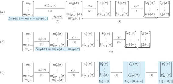
isnotrealisable.

3.2.Anewprocedurebasedonmomentrealisability

The reversiblelinear systemlinking raw moments ofthe approximation m

e

N to its degenerated moments m∗N is such

thatanewobjectivefunction D∗

N

(

σ

)

–whoserootisthesameasthatofDN

(

σ

)

–canbeformulated.Itscomputationisas

follow(seealsoFig.1b): 1. Computem∗

N

(

σ

)

=

A−N1

(

σ

)

·

mN.

2. Computeaquadratureonthevectorm∗_N−1

(

σ

)

toobtainthevectorswP

(

σ

)

and

ξ

P

(

σ

)

.

3. Computem∗_N

(

σ

)

=

P

iP₌1wi

(

σ

)ξ

i

(

σ

)

N.

4. ComputeD∗

Fig. 1. Comparisonofthecomputationofconvergencecriteriabasedon(a)DN(σ),(b)D∗

N(σ)and(c)therealisabilitycriteriaofthesupportÄξ.CA:

Chebyshev Algorithm. QC: Quadrature Computation. The convergence criteria are highlighted in light blue. Inspired by Fig. 1 from Nguyen et al. [1]. (For interpretationofthecoloursinthefigure(s),thereaderisreferredtothewebversionofthisarticle.)

Notethat DN

(

σ

)

=

D∗

N

(

σ

)

×

AN,N

(

σ

)

.As showninAppendixBforallkernels,diagonal elementsof An

(

σ

)

arealways

strictlypositive,thereforethetwoobjectivefunctionsdosharethesameroots.

Thebenefitofthisnewobjectivefunctionisthatitonlyrequiresthematrix A−_N1

(

σ

)

insteadofboththematrixA−_N−1₁

(

σ

)

andthelastlineofAN

(

σ

)

.Thisonlyincreasestheclarityofthemethod,buthashardlynoeffectonitsnumericalcost.

Thepoint ofthisalternativeapproachishowevertounderlineacrucialelementforthenewEQMOM implementation: we actually look fora value of

_σ

for whichm∗

2P

(

σ

)

=

m∗2P

(

σ

)

.This impliesthat, forthisspecific searched

σ

value, the

vectorm∗ 2P

(

σ

)

reads m∗_2P

(

σ

) =















P

P i₌1wi

ξ

_i0

P

P i₌1wi

ξ

_i1

..

.

P

P i₌1wi

ξ

i2P















(18)

whichis,byconstruction,thevectorofthefirst2P

₊

1 momentsofthesumof P Diracdistributions.

Under thecondition that a P -node EQMOM reconstruction exists forthemoment setm2P with

σ

>

0

,

wi

>

0

, ξ

i

6=

0

,

i

_{∈ {}

1

,

. . . ,

P

_}

,thevectorm∗

2P

(

σ

)

willhavethefollowingspecificproperties:

1. Thevectorm∗_2P−1

(

σ

)

mustbestrictlywithintherealisablemomentspace

M

_N−1

(Ä

ξ

)

. 2. Thevectorm∗

2P

(

σ

)

mustbeontheboundaryoftherealisablemomentspace

M

N

(Ä

ξ

)

.

EQMOM procedurewillthen relyontherealisabilityofthevector m∗_2P

(

σ

)

insteadofthecomputation oftheerroron thelastmoment,thiswillbeacheaperapproach.

Situations were the EQMOM reconstruction exist but with

_σ

₌

0, or

_∃

i

_{∈ {}

1

,

. . . ,

P

_},

wi

₌

0 or

ξ

i

=

0 are tackled in

section3.6butarealwaysbasedoncheckingtherealisabilityofm∗

2P

(

σ

)

.

The actual definition of the realisable moment space of order n,

M

_n, depends on the support

Ä

ξ of the NDF.The three classical supports, corresponding to the Hamburger,Stieltjes and Hausdorff momentproblems, comewith different constraints on a moment set to ensure its realisability.The realisabilitycriteria foreach ofthese supports will then be detailed.

Fig. 1sums up the“standard approach” based on DN

(

σ

)

,the shifted approach,based on D∗N

(

σ

)

, aswell asthe new

approachbasedontherealisabilitycriteriaofm∗_2P

(

σ

)

forallthreesupports.

3.3. Applicationtothe Hamburgerproblem

As stated in 2.2, it is known that monic polynomials which are orthogonal to a measure d

µ

(ξ )

=

n

(ξ )

d

ξ

satisfy a three-termrecurrencerelation(Eq.(5))withakandbk

,

k

∈ N

,therecurrencecoefficientsspecifictothemeasured

µ

(ξ )

.The

Favard’stheorem[31] andits converse[32] implythatthemeasure d

µ

(ξ )

isrealisableon

Ä

ξ

=

]

−∞, +∞

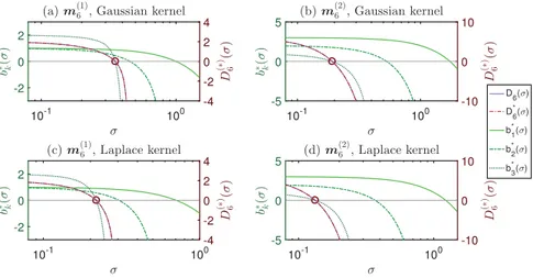
[ ifandonlyif

Fig. 2. EvolutionofthedifferentconvergencecriteriaforbothGaussian(aandb)andLaplace(candd)kernelsdependingonσ value.Thetwoinitial momentsetsarem(1)₆ = [1 1 2 5 12 42 133]T_andm(2)

6 = [1 2 7 17 58 149 493]T.

Onelooksforavalueof

_σ

suchthattheassociateddegeneratedmomentsm∗

2P−1

(

σ

)

arestrictlyrealisable(i.e.withinthe

momentspace),andthemomentsm∗

2P

(

σ

)

areweaklyrealisable(i.e.onthefrontierofrealisability).Then,iftheChebyshev

algorithmisusedtocomputetherecurrencecoefficientsa∗

P₋1

(

σ

)

= [

a∗0

(

σ

),

. . . ,

a∗P₋1

(

σ

)]

Tandb∗P

(

σ

)

= [

b∗1

(

σ

),

. . . ,

b∗P

(

σ

)]

T

fromthevectorm∗_2P

(

σ

)

,theconditionofrealisabilitycanbewrittenintermsofvaluesofb∗P

(

σ

)

:lookingfortheEQMOM

reconstructionparameterswiththeGaussianandLaplacekernelsisequivalenttolookingforavalueof

_σ

suchas:

•

b∗

k

(

σ

)

>

0,

∀

k

∈ {

1

,

. . . ,

P

−

1

}

•

b∗

P

(

σ

)

=

0

Fig.2 makes use of the developmentsfrom AppendixB.1 and Appendix B.2,about theGaussian andLaplace kernels respectively,toshowtheevolutionofD6

(

σ

)

,D∗6

(

σ

)

andbk∗

(

σ

),

k

∈ {

1

,

2

,

3

}

fortwosetsof7 moments(P

=

3).Thisfigure

illustratesthe factthat indeedthe approachesbasedon DN

(

σ

)

, D∗N

(

σ

)

andb∗P

(

σ

)

areequivalent asthey sharethesame

circledroot.

Letdenote

_σ

k therootofbk

(

σ

)

.Onecannoticethattheroot

σ

klieswithintheinterval [0

,

σ

k₋1].Weactuallyobserved

theexistence ofall roots

_σ

k

,

k

∈ {

1

,

. . . ,

P

}

onnumerous(about106) randomlyselected momentsetsof N

+

1

=

13

mo-ments,andneverobservedan undefinedroot.Thegenerality ofthisobservationhasnot beenmathematicallyproved,but itseemsthatindeed

_σ

kisalwaysdefinedandalwaysliesin

σ

k

∈

[0

,

σ

k−1]

,

k

∈ {

2

,

. . . ,

P

}

.

σ

1isdefinedanalytically.

Thepreviousobservationswereusedtodesignasimplealgorithmwhichallowsidentifyingtheroot

_σ

P.Thisalgorithm

isbasedonthefactthatitispossibletocheckwhetheravalue

_σ

t ishigherorlowerthan

σ

P atlowcostandwithnoprior

knowledgeof

_σ

P value:

•

Ifb∗

k

(

σ

t

)

>

0

, ∀

k

∈ {

1

,

. . . ,

P

}

,then

σ

t

<

σ

P.

•

Otherwise,thatisif

_∃

k

_{∈ {}

1

,

. . . ,

P

_},

b∗

k

(

σ

t

)

<

0,then

σ

t

>

σ

P.

Onecanthenuseaniterativeapproachthatwill

1. Check the realisability of the raw moments m2P

=

m∗2P

(

0

)

by computing b∗P

(

0

)

and checking the positivity of all

elements.

2. Initialiseaninterval

h

σ

_l(0)

,

σ

r(0)

i

suchthat

_σ

_l(0)

<

σ

P and

σ

r(0)

>

σ

P,andthenupdatetheseboundstoshrinkthesearch

interval.Theseinitialvalueswillbe

_σ

(0)

l

=

0 and

σ

(0)

r

=

σ

1with

σ

1 theanalyticalsolutionofb∗1

(

σ

)

=

0.

3. Iterateoverk (a) Choose

_σ

t

∈

h

σ

_l(k−1)

,

σ

r(k−1)

i

. (b) Computeb∗P

(

σ

t

)

.

(c) Ifallelementsofb∗P

(

σ

t

)

arepositive,set

σ

l(k)

=

σ

t and

σ

r(k)

=

σ

r(k−1).

(d) Otherwise,set

_σ

(k) l

=

σ

(k₋1) l and

σ

(k) r

=

σ

t.

Thechoiceof

_σ

t atstep3awillbemadeby tryingtolocatetheroot

σ

jofb∗_j

(

σ

)

with j theindexofthefirstnegative

elementof b∗_P

³

σ

r(k)

´

.Following Nguyenetal.[1] developments,the useofRidder’smethod isadvised toselect

_σ

t.This

3. Iterateoverk

(a) Identify j theindexofthefirstnegativeelementofb∗_P

³

σ

r(k−1)

´

. (b) Compute

_σ

t1

=

1 2

³

σ

_l(k−1)

+

σ

r(k−1)

´

andb∗P

(

σ

t1

)

. (c) Compute

_σ

t2

=

σ

t1

+

³

σ

t1

−

σ

(k₋1) l

´

b∗ j ¡ σ_t1¢ r b∗ j ¡ σ_t1¢2−b∗ j ³ σl(k−1) ´ ∗b∗ j ³ σr(k−1) ´ andb∗P

(

σ

t2

)

.

(d) Set

_σ

_l(k) asthe highest value between

_σ

_l(k−1),

_σ

t1 and

σ

t2 such that the corresponding vector b∗P contains only

positivevalues. (e) Set

_σ

(k)

r asthelowestvalue between

σ

r(k−1),

σ

t1 and

σ

t2 suchthat thecorresponding vector b∗P contains atleast

onenegativevalue.

Stop the computation if

_σ

r(k)

−

σ

l(k)

<

ε σ

1 or ifb∗P

³

σ

_l(k)

´

<

ε

b∗

P

(

0

)

, with

ε

a relative tolerance (e.g.

ε

=

10−10). Then

compute the weights wP andnodes

ξ

P of the EQMOM reconstruction by computing a Gauss quadrature based on the

recurrencecoefficientsa∗

P₋1

³

σ

_l(k)

´

andb∗_P−1

³

σ

_l(k)

´

.

Actualimplementationsofthisalgorithmforbothkernelsareprovidedassupplementarydata.

3.4. Applicationtothe Stieltjesproblem

It iswell known that therealisabilityofa momentset mN on thesupport

Ä

ξ

=

]0

, +∞

[ isstrictly equivalent to the positivityoftheHankeldeterminants

H

_2n

+d[33] definedas:

H

_2n +d

=

¯

¯

¯

¯

¯

¯

¯

md

· · ·

mn+d

..

.

. .

.

..

.

mn+d

· · ·

m2n+d

¯

¯

¯

¯

¯

¯

¯

(19) withd

∈ {

0

,

1

}

andn

∈ N,

2n

+

d

≤

N.

This condition on the positivity of Hankel determinants can be translated into a condition on the positivity of the numbers

ζ

k [32] definedby:

ζ

k

=

H

k−3

H

k

H

_k −2

H

k₋1

,

H

_j

₌

1 if j

<

0 (20)

ThesenumberscanbedirectlycomputedfromtherecurrencecoefficientsaP andbP definedin2.2throughthefollowing

relations:

ζ

2k

=

bk

ζ

2k−1

,

ζ

2k+1

=

ak

− ζ

2k (21) with

ζ

1

=

a0

=

m1

/

m0.

The goal here is to usethese realisabilitycriteria to compute the parameters ofEQMOM quadraturewith either the Log-normal, theGamma orthe Weibullkernel (seeAppendix B.3,Appendix B.4 andAppendixB.5 respectively). Inthese cases,onemust

1. Compute m∗_N

(

σ

)

=

A_N−1

(

σ

)

·

mN with AN

(

σ

)

the matrix associated to the chosen kernel (see Appendix B.3,

Ap-pendixB.4,AppendixB.5).

2. ApplytheChebyshevalgorithmtom∗

N

(

σ

)

toaccesstherecurrencecoefficientsa∗P

(

σ

)

andb∗P

(

σ

)

.

3. Compute

ζ

∗_N

(

σ

)

= [ζ

1∗

(

σ

),

. . . ,

ζ

N∗

(

σ

)]

TusingrelationsinEq.(21).

Oneactuallylooksfor

_σ

suchthat

• ζ

k∗

(

σ

)

>

0,

∀

k

∈ {

1

,

. . . ,

N

−

1

}

• ζ

N∗

(

σ

)

=

0

Let

_σ

kbetherootof

ζ

k∗

(

σ

)

.Inallcases,theroot

σ

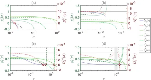
2isdefined,analyticallyfortheLog-normalandGammakernels,and

numericallyfortheWeibullkernel.Fig.3showstheevolutionof D6

(

σ

)

,D∗6

(

σ

)

and

ζ

∗6

(

σ

)

forthreemomentsetswhenthe

developmentsrelativetotheWeibull(seeAppendixB.5)kernelareused.Threesituationscanbeobservedonthatfigure: 1. Allroots

_σ

k,k

∈ {

2

,

. . . ,

N

}

aredefined(Fig.3a).

2. Someintermediaryroots

_σ

k,k

∈ {

3

,

. . . ,

N

−

1

}

,arenotdefinedbuttheroot

σ

N stillexists(Fig.3b).

252

Fig. 3. Evolution of the different convergence criteria for the Weibull kernel depending on σ value. The initial moment sets are m(6a)= [1 1.5 12 131 15200 18033 2.16e5]T_,m(b)

6 = [1 5.5 78 1285 22225 4.05e5 7.88e6]Tandm (c)

6 = [1 1 2 5 14 42 133]T.

ThesethreecasescanbeobservedfortheGammaandLog-normalkernelstoo.

Inthefirsttwocases,when

_σ

N exists,theEQMOMapproximationiswelldefined.Thelast case–where

ζ

_N∗

(

σ

)

admits

norootin[0

,

σ

N₋1] –actuallycorrespondstothecasedescribedbyNguyenetal.[1] whereDN

(

σ

)

didnotadmitanyroot

either.Inthiscase,itwassuggestedtominimiseDN

(

σ

)

inordertoreducethedifferencebetweenmN andmN

e

(

σ

)

asmuch aspossible.

DN

(

σ

)

tendstobeadecreasingfunction,butisundefinedassoonasanyelementof

ζ

∗

N−1

(

σ

)

isnegative.Theminimum

ofDN

(

σ

)

isthenusuallylocatedatthehighestorderdefinedroot.Forinstance,inthecaseshowninFig.3c,theminimum

ofD6

(

σ

)

islocatedattheroot

σ

5 of

ζ

5∗

(

σ

)

.

Themoment-inversionprocedureforreconstructionkernelsdefinedon

Ä

ξ

=

]0

, +∞

[ isthenreducedtothe identifica-tionofthedefinedroot

_σ

k

,

k

∈ {

2

,

. . . ,

N

}

,ofhighestindex.Thealgorithmproposedinsection3.3alreadyconvergestoward

thisrootandonlyrequireslittleadjustments:

1. Check the realisability of the raw moments m2P

=

m∗2P

(

0

)

by computing

ζ

∗N

(

0

)

and checking the positivity of all

elements.

2. Initialiseaninterval

h

σ

_l(0)

,

σ

r(0)

i

with

_σ

_l(0)

₌

0 and

_σ

r(0)

=

σ

2with

σ

2 thesolutionof

ζ

2∗

(

σ

)

=

0.

3. Iterateoverk

(a) Identify j theindexofthefirstnegativeelementof

ζ

_N∗

³

σ

r(k−1)

´

. (b) Compute

_σ

t1

=

1 2

³

σ

_l(k−1)

+

σ

r(k−1)

´

and

ζ

∗ N

(

σ

t1

)

. (c) Compute

_σ

t2

=

σ

t1

+

³

σ

t1

−

σ

(k₋1) l

´

ζ∗ j ¡ σ_t1¢ r ζ∗ j ¡ σ_t1¢2−ζ∗ j ³ σ_l(k−1)´∗ζ∗ j ³ σr(k−1) ´ and

ζ

∗N

(

σ

t2

)

. (d) Set

_σ

(k)

l as the highestvalue between

σ

(k₋1)

l ,

σ

t1 and

σ

t2 such that the corresponding vector

ζ

∗N contains only

positivevalues.

(e) Set

_σ

r(k) asthelowestvalue between

σ

r(k−1),

σ

t1 and

σ

t2 suchthat thecorresponding vector

ζ

∗N containsatleast

onenegativevalue. Stopthecomputationif

_σ

r(k)

−

σ

(

k)

l

<

εσ

1orif

ζ

N∗

³

σ

_l(k)

´

<

ε

ζ

∗

N

(

0

)

,with

ε

arelativetolerance(e.g.

ε

=

10−10).Thencompute

the weights wP and nodes

ξ

P of the EQMOM reconstruction by computing a Gaussian-quadrature based on recurrence

coefficientsa∗ P−1

³

σ

_l(k)

´

andb∗ P₋1

³

σ

_l(k)

´

.

3.5.Applicationtothe Hausdorffproblem

Momentsof adistribution definedon theclosed support

Ä

ξ

=

]0

,

1[ mustobey two setsof conditionsinorderto be withintherealisablemomentspace[15,26].ThemomentsetmN isinteriortotherealisablemomentspaceassociatedto

thesupport

Ä

ξ

=

]0

,

1[ ifandonlyif:

• H

k

>

0,

∀

k

∈ {

0

,

. . . ,

N

}

Fig. 4. EvolutionofthedifferentconvergencecriteriafortheBetareconstructionkernelandfourinitialmomentsets.Thesesetscanbefoundinthefigure sourcecodeprovidedassupplementarydata.

with

H

_kdefinedinEq.(19) and

H

_kdefinedby

H

_2n +d

=

¯

¯

¯

¯

¯

¯

¯

md−1

−

md

· · ·

mn+d−1

−

mn+d

..

.

. .

.

..

.

mn+d−1

−

mn+d

· · ·

m2n+d−1

−

m2n+d

¯

¯

¯

¯

¯

¯

¯

(22)

Leavingasidetheobviouscondition

H

₀

₌

m0

>

0,theconditions

H

k

>

0 and

H

k

>

0 inducealowerboundm−k andan

upperboundm+_k forthevaluesofmk,k

∈ {

1

,

. . . ,

N

}

.Consequently,onecandefinethecanonicalmomentsofthedistribution

pN

= [

p1

,

. . . ,

pN

]

Tas

pk

=

mk

−

m−k

m+_k

−

m−_k (23)

AmomentsetmN isstrictlyrealisableifandonlyiftheassociatedcanonicalmomentset pN liesinthehypercube]0

,

1[N.

Canonicalmomentscanbecomputedthroughtherecurrencerelation[34]:

pk

=

ζ

k

1

₋

pk₋1

(24)

with

ζ

kdefinedinEq.(20) andp1

=

m1.

Inthe caseoftheBetakernel(see B.6),one islookingfora value of

_σ

such thatthe vector p∗

N

(

σ

)

hasthe following

properties:

•

p∗

k

(

σ

)

∈

]0

,

1[

,

∀

k

∈ {

1

,

. . . ,

N

−

1

}

•

p∗

N

(

σ

)

=

0

p∗_N

(

σ

)

iscomputedfromthevector

ζ

∗_N

(

σ

)

whichisdeducedfromtherecurrencecoefficientsa∗_P−1

(

σ

)

andb∗P

(

σ

)

.These

arecomputed–likepreviously– throughtheChebyshevalgorithmappliedtothevectorm∗

N

(

σ

)

=

A−

1

N

(

σ

)

·

mN.

Fig.4showstheevolutionofthecanonical momentsandtheconvergencecriteriaD6

(

σ

)

andD∗6

(

σ

)

forfourdifferent

setsof7momentswiththedevelopmentsrelativetotheBetakernel(seeAppendixB.6).Eachofthesesetscorrespondsto oneofthefoursituationsencounteredwhendealingwithBetaEQMOM:

•

Fig.4a: theroot

_σ

N of DN

(

σ

)

, D∗N

(

σ

)

andp∗N

(

σ

)

existsandcan beidentified througha similarprocedure thanthat

describedinsections3.3and3.4.

•

Fig.4b:theroot

_σ

N isnotdefinedbuttheminimumofDN

(

σ

)

islocatedatthe

σ

valueforwhich p∗_N−1

(

σ

)

isonthe

boundaryofthehypercube]0

,

1[N−1_.

•

Fig.4c: DN

(

σ

)

,D∗N

(

σ

)

andp∗N

(

σ

)

admitmultipleroots.

•

Fig.4d: theroot

_σ

N isdefined,butthereis arange

]

σ

v1

,

σ

v2

[

with

σ

v2

<

σ

N,highlighted inlightgrey, suchthat in

Thealgorithm proposed insections 3.3and3.4can still be applied hereby replacingthe convergencecriteriaby the canonical moments, and by checking that the values of p∗

N

(

σ

)

all lie inthe interval ]0

,

1[ instead of checkingonly for

positivity:

1. Checktherealisabilityoftherawmoments m2P

=

m∗2P

(

0

)

bycomputing p∗N

(

0

)

andcheckingthat allelements liein

]0

,

1[. 2. Initialiseaninterval

h

σ

_l(0)

,

σ

r(0)

i

with

_σ

(0) l

=

0 and

σ

(0)

r

=

σ

2with

σ

2 theanalyticalsolutionof p∗2

(

σ

)

=

0.

3. Iterateoverk

(a) Identify j theindexofthefirstelementof p∗

N

³

σ

r(k−1)

´

thatiseithernegativeorhigherthan1. (b) Compute

_σ

t1

=

1 2

³

σ

_l(k−1)

+

σ

r(k−1)

´

and p∗ N

(

σ

t1

)

. (c) If j

<

N and p∗ j

³

σ

r(k−1)

´

>

1

•

Compute

_σ

t2

=

σ

t1

+

³

σ

t1

−

σ

(k₋1) l

´

q∗ j ¡ σ_t1¢ r q∗ j ¡ σ_t1¢2−q∗ j ³ σl(k−1) ´ ∗q∗ j ³ σr(k−1) ´ andp∗N

(

σ

t2

)

,withq∗j

(

σ

)

=

1

−

p∗j

(

σ

)

. (d) Else,thatisif j

₌

N orp∗ j

³

σ

r(k−1)

´

<

0

•

Compute

_σ

t2

=

σ

t1

+

³

σ

t1

−

σ

(k₋1) l

´

p∗ j ¡ σ_t1¢ r p∗ j ¡ σ_t1¢2−p∗ j ³ σl(k−1) ´ ∗p∗ j ³ σr(k−1) ´ and p∗N

(

σ

t2

)

.

(e) Set

_σ

_l(k) asthehighestvaluebetween

_σ

_l(k−1),

_σ

t1 and

σ

t2 suchthatthecorrespondingvector p∗N liesin]0

,

1[ N_.

(f) Set

_σ

r(k) asthe lowest value between

σ

r(k−1),

σ

t1 and

σ

t2 such that the corresponding vector p∗N doesnot lie in

]0

,

1[N_.

Stopthecomputation if

_σ

r(k)

−

σ

l(k)

<

εσ

2 orif p∗N

³

σ

_l(k)

´

<

ε

p∗

N

(

0

)

,with

ε

arelative tolerance(e.g.

ε

=

10−10). As

previ-ously,onceconvergenceisachieved,theweights wP andnodes

ξ

P ofthereconstructioncanbeobtainedbycomputinga

Gaussianquadraturerulebasedontherecurrencecoefficientsa∗

P₋1

³

σ

_l(k)

´

andb∗_P−1

³

σ

_l(k)

´

.

Thisalgorithm willconvergetotheroot

_σ

N forcasessimilar toFig.4a; totheminimumofDN

(

σ

)

forcasessimilarto

Fig.4b;tooneofthemultiplerootsforcasessimilartoFig.4c.InthecaseillustratedinFig.4d,thealgorithmmayormay notidentifytheexistingroot,dependingonwhetheroneoftheintermediatetested

_σ

valuesliesinthegreyedarea.

Onecouldtrytodevelopamorerobustalgorithm,thatwillalwaysfindtherootifitisdefined,eveninthecaseshownin Fig.4d.Anotherimprovementwouldbetoensureaconsistentresultwhenmultiplerootsexist,forinstancebyconverging towardthelowestroot,sothatasmallperturbationintherawmomentswillonlycauseasmallchangeontheresulting

_σ

value.Nothingpreventsthecurrentalgorithmfromconvergingtowardonerootforamomentsetandtowardanotherone afterasmallperturbationofthissetwhichcouldinduceinstabilitiesinlarge-scalesimulations.Notethattheselimitations alreadyexistedinpreviousEQMOMimplementationsanddonotresultfromthenewapproachdevelopedinthisarticle.

3.6.Handlingweaklyrealisableandill-conditionedmomentsets

TheEQMOMmoment-inversionprocedureattemptstoidentifyaNDFdefinedby

e

n

_{(ξ ) =}

P

X

i₌1

wi

δ

σ

(ξ, ξ

i

)

(25)

whosefirst2P

₊

1 integermomentsaregivenbym2P.

Thisapproximationisnotalwayspossibleasshowninsections3.4and3.5.WhentheEQMOMapproximationexists,it maybeill-conditionedifatleastoneofthefollowingsholdstrue:

•

σ

=

0

• ∃

i

,

wi

₌

0

• ∃

i

, ξ

i

=

0

Thefirst situationis that ofm2P beingweakly realisable. The second situationoccursif m2P is the momentset ofa

convexmixture ofthe reconstructionkernelwithlessthan P nodes.Thesesituationsarenot mutuallyexclusive,a vector m6couldbethevectorofthe7firstmomentsofabi-Diracdistribution,oneofwhichcouldbelocatedin

ξ =

0.

Accountingfor thesesituations requiresintroducing the orderofrealisability ofa momentset,

N (

mN

)

.This notation

wasintroducedbyNguyenetal.[1] butwasonlydefinedon

Ä

ξ

=]

0

,

+∞[

intermsofHankeldeterminants.Thefollowing definitionisbroaderasit encompassestheirsbutextendsitto othersupports.

N (

mN

)

isthenumberofmomentsinthe

largeststrictly realisablesubset ofmN.Foreach support,the orderof realisabilityisdefinedinterms ofthe realisability

•

For

Ä

ξ

=

]

−∞, +∞

[,computebP fromm2P;

– ifallelementsarepositive,

N (

m2P

)

=

2P

₊

1; – else,ifthereisn suchthatbn

=

0,

N (

m2P

)

=

2n;

– else,ifthereisn suchthatbn

<

0,

N (

m2P

)

=

2n

−

1.

•

For

Ä

ξ

=

]0

, +∞

[,compute

ζ

2P fromm2P;

– ifallelementsarepositive,

N (

m2P

)

=

2P

+

1;

– elseidentifyn suchthat

ζ

n

≤

0,

N (

m2P

)

=

n.

•

For

Ä

ξ

=

]0

,

1[,compute p2P fromm2P;

– ifallelementsareincludedon

_]

0

,

1

_[

,

N (

m2P

)

=

2P

+

1;

– elseidentifyn suchthat pn

∈ ]

/

0

,

1

[

,

N (

m2P

)

=

n.

Detecting situationswhere

_σ

₌

0 requires tocheck the orderofrealisability ofrawmoments. If

N (

m2P

)

iseven, set

σ

=

0;otherwiseapplytheiterativeproceduretom2P′ with

N (

m2P

)

=

2P′

₋

_{1 toidentify}

_σ

_[1].

The actual numberof nodesrequired by the EQMOM approximation, i.e. the numberof non-zero weights P′′_{, is} de-termined from

N (

m∗_2P

(

σ

))

.Ifit is even, P′′

_{= N (}

_m∗

2P

(

σ

))/

2; otherwise, P′′

= (N (

m2P∗

(

σ

))

+

1

)/

2 but one node willbe

locatedin

_{ξ =}

0 whichmightbeanissueforKDFsdefinedon

Ä

ξ

=

]0

, +∞

[ or

Ä

ξ

=

]0

,

1[.Theweightsandnodeswillbe computedfromtherecurrencecoefficientsa∗

P′′₋1

(

σ

)

andb∗P′′₋1

(

σ

)

.If P′′

<

P ,let wk

=

0

,

ξ

k

=

1

/

2

, ∀

k

∈ {

P′′

+

1

,

. . . ,

P

}

.

Theseadjustments ofthe firstandlaststeps ofalgorithmsdescribed insections3.3,3.4and3.5give greatstability to themoment-inversionprocedureatlowcost.

Inthesituationwhere

N (

m∗

2P

(

σ

))

=

2P ,theEQMOMapproximationis guaranteedtopreservethe wholemomentset m2P.However, if

N (

m∗_2P

(

σ

))

<

2P ,theapproximationmay,ormaynot,preserveall momentswithnosimplemethodto

checkforthis.OneshouldcomputethemomentsoftheEQMOMapproximationandmeasuretherelativeerrorfromoriginal moments.

4. ComparisonofEQMOMapproaches 4.1. Method

The new EQMOM moment-inversionprocedure only requirescomputation ofthe realisabilitycriteriaof the vector of degeneratedmomentsm∗

2P

(

σ

)

inordertoidentify

σ

.Thesecomputationswerealreadyperformedintheoriginalapproach

[1] toensuretherealisabilityofthevectorm∗_2P−1

(

σ

)

priortothequadraturecomputationandulteriorsteps.

Itisthereforeobviousthatthenewapproachwillalwaysrequirealowernumberoffloatingpointoperations(FLOP).In orderto quantifythisreductiononFLOP number,andtheactual performancegain, differentimplementationsofEQMOM arecompared,theyarebasedeitherontherealizabilitycriteria,oronaquadrature-basedobjectivefunction.

4.1.1. TestedEQMOMimplementations

Comparisonareperformedforkernelsdefinedon

Ä

ξ

=

]

−∞, +∞

[ (i.e.GaussandLaplacekernels),andon

Ä

ξ

=

]0

, +∞

[ (i.e.Log-Normal,GammaandWeibullkernels),usingMATLAB[22] implementations.

Implementationsthat arebasedontherealizabilitycriteriaofm∗

2P

(

σ

)

usealgorithms thatwerefullydescribedin

sec-tions3.3and3.4andadjustmentsfromsection3.6.

For quadrature-based moment-inversion implementations, we optimized codes fromMarchisio and Fox [20] and the OpenQBMM project[19] byimplementingoptimizationssuggestedbyNguyen etal.[1] andadjustmentsfromsection3.6. InsteadofsearchingfortherootofD2P

(

σ

)

(seeFig.1a),theseimplementationsdirectlysearchtherootofD∗2P

(

σ

)

(Fig.1b).

Doingso,allcomparedimplementationsonlyrequirethematrix A_2P−1

(

σ

)

andcanbenefitfromthesamecodeoptimization whencomputingm∗_2P

(

σ

)

=

A_2P−1

(

σ

)

·

m2P.

For kernels definedon

Ä

ξ

=

]0

, +∞

[, ifRidder’s methodfails to identifya root of D∗2P

(

σ

)

, the golden-ratio method

is usedtominimize D2P

(

σ

)

2

=

¡

D∗2P

(

σ

) ·

A2P,2P

(

σ

)

¢

2.Thegolden-ratiominimization methodwas alreadyusedin

Open-QBMM [19].

4.1.2. Performancemeasurements

The mainelement ofcomparisonis thenumberoffloating-pointoperationsrequiredforthewhole moment-inversion procedure. The MATLAB implementations embed a simple FLOP counter that distinguishes each operation (

+

,

−

,

∗

,

/

, exp,

√

_·

,

_Ŵ(·)

,. . . )andcountsthemforeachstepofthemoment-inversionprocedure(linearsystem, Chebyshevalgorithm, quadraturecomputationandothers).

InordertoevaluatethenumberofoperationsusedinthecomputationoftheeigenvaluesandeigenvectorsoftheJacobi matrix(Eq.(6)),theJacobiandtheFrancisalgorithmswhicharesuitedforsymmetricmatrices[35] areusedinplaceofthe MATLABbuilt-in“eig”function[22].TheJacobialgorithmisusedformatricesofsizeupto3

_×

3 andtheFrancisalgorithm forlargermatricesinordertoalwaysusethefastestmethod.

Twoothersmetricsaremeasuredforeachcalltothemoment-inversionprocedure:thenumberoftested

_σ

valuesand thewall-timeoffunctioncalls.

Table 1

ComparisonofGaussEQMOMimplementationscorrespondingtoFig.1band1c formomentsetsfarfromthefrontierofrealisability.ThecountofFLOP detailstheoperationsrelatedto(i)thematrix–vectorproductA−1

2P(σ)·m2P,(ii)theChebyshevAlgorithm(CA),(iii)theQuadratureComputation(QC)and

(iv) amiscellaneouscategory.Resultsaregivenasmean±standard-deviationamong104_momentsets.

P=2 P=3 P=4 P=5 New approach FLOP A−2P1(σ) 237±59 767±141 1709±253 3201±476 CA 177_±40 477±83 979±139 1751±251 QC 52_±0 474±42 995±120 1746±188 Misc. 54_±12 65±11 75±11 86±12 Total 519_±112 1783±242 3759±441 6784±830 Evaluations 12_±3 14±2 17±2 19±3 Run-time (ms) 1_±0 2±0 3±0 4±1 Former approach FLOP A−2P1(σ) 295±161 1433±423 4060±869 8516±1870 CA 202±102 853±241 2246±467 4509±967 QC 742±377 9171±2910 24997±9966 52312±14096 Misc. 191_±99 430±129 804±156 1298±251 Total 1429_±739 11887±3603 32108±10645 66635±16085 Evaluations 14±7 26±7 39±8 50±11 Run-time (ms) 1_±1 9±3 17±5 31±7 Gain in FLOP 59.1%_±12.3% 84.2%_±3.5% 87.9%_±2.5% 88.0%_±13.1% Evaluations 8.6%_±27.7% 40.9%_±17.7% 54.2%_±12.8% 53.0%_±55.2% Run-time 53.2%_±13.2% 81.9%±4.2% 84.0%±3.6% 83.3%±18.0%

4.1.3. Testedmomentsets

Eachcomparisonwasperformedon104 _{randomlygeneratedmomentsets.Thesehavevaryingsize2P}

+

1

_{∈ {}

5

,

7

,

9

,

11

_}

andwereeitherfarfrom,orcloseto,theboundaryoftherealisablemomentspace.

Momentssets forkernels definedon

Ä

ξ

=

]

−∞, +∞

[ were computedfromrandomvectorsaP₋1 andbP using a

re-versedChebyshevalgorithm.Distributionlawsfortheelementsofthesevectorsare

•

ak

∼ N (

0

,

25

),

k

∈ {

0

,

. . . ,

P

−

1

}

.

•

bk

∼

1

+

Exp

(

4

),

k

∈ {

1

,

. . . ,

P

}

.

•

bP

∼

Exp

(

0

.

5

)

formomentsetsclosefromthefrontierofrealisability.

Similarly,momentssetsforkernelsdefinedon

Ä

ξ

=

]0

, +∞

[ werecomputedfromrandomvectors

ζ

2P usingareversed

ζ

-Chebyshevalgorithm[1].Elementsofthesevectorsaregeneratedusingfollowingdistributionlaws:

• ζ

k

∼

1

+

Exp

(

4

),

k

∈ {

1

,

. . . ,

2P

}

.

• ζ

2P

∼

Exp

(

0

.

5

)

formomentsetsclosefromthefrontierofrealisability.

4.1.4. Reproducibility

Toallowreproducibilityofresultsdescribedhereafter,everysourcecodespreviouslydescribed,andrandomlygenerated data,areavailableassupplementarydata.

4.2.Results

ResultsofthecomparisonperformedonGauss-EQMOMformomentsetsfarfromtheboundaryoftherealisablemoment spacearegiveninTable1.Similartablesareavailableassupplementarydataforallkernelsandmomentsets.

Table2underlinesadecreaseinthenumberoftested

_σ

values,inparticularforhighorderreconstructions.Thisdecrease ismainlydueto thefactthatintheformerapproach,ifm∗_N−1

(

σ

)

turnsout nottoberealisable, theobjectivefunctionis settoa arbitrarilyhighnegative value. Theuseofsuch anarbitraryvalue slowsdownthe convergenceofthenon-linear equation solver. Meanwhile, the new approach never makes use of arbitrary values, all the elements of the vectors of realisabilitycriteria(b∗

P

(

σ

)

,

ζ

∗2P

(

σ

)

or p∗2P

(

σ

)

)areusedoneaftertheotherwhichyieldsabetterchoiceofthenexttested

σ

value.

Moreover,forkernelsdefinedon

Ä

ξ

=

]0

, +∞

[ andinsituationsillustratedinFig.3c,theformerapproachmayswitch froma rootsearch toa minimization processif norootis found.Thisinduces numerous supplementary tested

_σ

values beforeconvergenceisreachedwhilethissituationneveroccursinthenewapproach.

Asignificant dropin thetotal numberofFLOP can be observedin Table3.This was expectedandismainly justified bythefactthat thequadraturecomputation isonlycalledonce inthenewapproachwhilstitiscalledformosttested

_σ

valuesintheformermoment-inversion procedure.Thisquadrature,whichconsistsinthe computationofthe eigenvalues