an author's https://oatao.univ-toulouse.fr/23022
Boyer, Marc and Daigmorte, Hugo and Navet, Nicolas and Migge, Jörn Performance impact of the interactions between time-triggered and rate-constrained transmissions in TTEthernet. (2016) In: 8th European Congress on Embedded Real Time Software and Systems, 31 January 2016 - 2 February 2016 (Toulouse, France).
Performance impact of the interactions between time-triggered
and rate-constrained transmissions in TTEthernet
Marc Boyer, ONERA, France Hugo Daigmorte, ONERA, France Nicolas Navet, University of Luxembourg
Jörn Migge, RealTime-at-Work, France
Abstract: Switched Ethernet is becoming a de-facto standard in industrial and embedded networks. Many
of today’s applications benefit from Ethernet’s high bandwidth, large frame size, multicast and routing capabilities through IP, and the availability of the standard TCP/IP protocols. There are however many variants of Switched Ethernet networks, just considering the MAC level mechanisms on the stations and communication switches. An important technology in that landscape is TTEthernet, standardized as SAE6802, which allows the transmission of both purely time-triggered (TT) traffic and sporadic (or rate-constrained - RC) traffic. To the best of our knowledge, the interactions between both classes of traffic have not been studied so far in realistic configurations. This work aims to shed some light on the kind of performances, in terms of latencies, jitters and useful bandwidth that can be expected from a mixed TT and RC configuration. The following issues will be answered in a quantified manner by sensitivity analysis: How do both classes of traffic interfere with each other? What are the typical worst-case latencies and useful bandwidth that can be expected for a RC stream for various TT traffic loads? What is the overall impact of TTEthernet integration policy for the RC traffic? This study builds on a worst-case traversal time analysis developed by the authors for SAE6802, and explores these questions by experiments performed configurations of various sizes.
Keywords: Time-Triggered Ethernet, worst-case traversal times, sensitivity analysis, benchmarking.
1 T T E t h e r n e t : t r a n s m i s s i o n s c h e d u l e f o r s e v e r a l c l a s s e s o f t r a f f i c
The SAE standard AS6802, [AS6802] describes a network called Time-Triggered Ethernet, also known as
TTEthernet [Ste09]. As explained in the standard, AS6802 “adds synchronization and time-deterministic data transfer characteristics to those Ethernet operations that use active star (e.g., hub or switch) topologies, while retaining full compatibility with the requirements of IEEE 802.3” [AS6802]. In fact, while
keeping the same frame format as IEEE 802.3, AS6802 defines three kinds of data flows:
– A time-triggered (TT) traffic, where a global (periodic) time schedule defines for each TT flow the time point at which frames have to be sent.
– A rate constrained (RC) traffic, where each flow has a bandwidth limit defined by two parameters: a minimal duration between two successive frames at the source and a maximal frame size. This constraint is the same as the one of ARINC664 P7, also known as AFDX (Avionics Full DupleX ethernet), where this minimal duration is called a BAG (Bandwidth Allocation Gap).
– A best-effort (BE) traffic that is simply a class for low-priority Ethernet traffic without timing and delivery guarantees.
Both TT and RC flows are statically defined, with a single source, a static routing, and a set of receivers.
Figure 1: Topology and data flow example.
Let us consider the system shown in Figure 1 with a single switch connecting four nodes, S1, S2, R1, and R2. The node S1 sends two flows, F1 to R2 and F2 to R1, while the node S2 sends one flow, F3 to R2. Let us assume that F2 and F3 have the same period P, and F1 a period equal to 2⋅P.
Sending all flows as TT traffic requires building a global frame schedule for all links such that there is no contention, and, in the best case, no buffering of frames in switches (a frame is sent as soon as it is received). Such a schedule is given in Figure 2.
Figure 2: Schedule example with purely TT traffic.
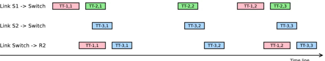
With purely RC traffic, no synchronization is needed between the nodes, what is required is only the respect of the per-flow inter-frame gap in emission. Then, some contention can occur in the switches, and frames have to be buffered. This buffering adds some jitters to the flow. For instance in the example of Figure 3, even if the flow F3 is sent with a periodic pattern, the interference can shorten the distance between two successive messages (see messages RC-3,1 and RC-3,2).
Figure 3: Schedule example with purely RC traffic.
At first sight, TT traffic seems a better solution than RC traffic, but it requires a lot of care. The first obvious point is that it requires a global clock, and a large part of the SAE standard consists in defining a robust protocol for global synchronization. It implies the addition of “protocol control frames” (PCF). A second requirement is the ability to build a global communication schedule, which is a NP-complete problem. Generating communication schedule involves non-trivial optimization algorithms, see for instance [Ta13], whose actual performances are difficult to assess given that no optimal solution can be known except on very small problems. Lastly, the best temporal performances are achieved when synchronizing the tasks schedule and the communication schedule. Actually, the network is meant to transfer data between tasks, and the delay to control is the delay between data production and data consumption. Indeed, without synchronization between the tasks and the network, a data may have to wait a full transmission period before being sent. Similar asynchronisms can create latencies in reception too. This means that, if the local scheduling on a computer is changed during the design process of a system, it may impact the network scheduling and then the scheduling on all computers.
On the opposite, a RC traffic does not require a global synchronization. It also requires some analysis method, not to build the global schedule, but to verify that the system’s timing behavior will respect the memory and frame latency constraints (see [Gr04, Fr06, Bo11] for switched Ethernet networks). An important property of the RC traffic is that the frame communication delays can be computed independently of the task scheduling on the sending station. This means that changing the task scheduling on a station will not have any impact on the other nodes as long as long as the constraint of the minimum time between two successive transmissions is met.
Because not all streams have the same transmission requirements, and because development constraints may prevent the use of TT traffic for some nodes, it can be a practical solution to take advantage of the AS6802 protocol flexibility and mix on the same network TT and RC traffic as illustrated on Figure 4. But mixing both kinds of traffic1 implies interferences. Each TT frame is scheduled for transmission on a link at a specific time point, whereas an RC frame can be sent almost at any time, creating thus interferences at the
1 The standard actually supports three kinds of traffic: TT and RC, but also Best Effort (BE) traffic. This latter class that comes without any guarantee with respect to delays and even proper frame delivery will be ignored in this paper.
link access level. The SAE standard defines two integration policies for the RC and TT traffic in the communication switches: shuffling and preemption [AS6802], whereas former works have considered also
timely block and resume preemption [Ste09]:
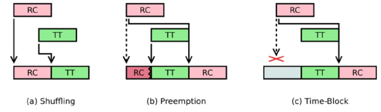
– In case of shuffling, an RC frame can be sent at any time, and the transmission of TT frame is postponed so that the RC frame can complete its transmission. Then, a TT is no more associated to a time instant (called scheduled point in time) but to a time window, the scheduled window2. – In case of preemption, when a TT frame has to be sent, the sender aborts the transmission of the RC
frame in order to send the TT frame immediately. The RC frame is sent again after the TT frame, from the start (this is called preemption restart).
– The timely block idea is to block any RC frame emission if its emission time can interfere with the next TT frame.
– The resume preemption mechanism consists in resending the frame from where it was stopped, and not from the start. These two latter mechanisms have not been kept in the standard.
In case of preemption, the low jitter and low latency of the TT traffic is favored over the RC one, but some bandwidth is lost and RC traffic latencies increase. On the opposite, in case of shuffling, no bandwidth is lost but the TT traffic will experience a larger latency.
Figure 4: TT-RC integration policies.
Two RC-TT traffic integration policies are considered in this study: timely-block, which minimizes the jitters for the TT flows, and the shuffling integration policy which is work-conserving.
The global clock synchronization service is implemented through the exchange of dedicated frames. The SAE standard uses PCF (Protocol Control Frames) of small size (64 bytes) for this purpose. These PCF frames belong to some specific RC flows, with priority higher than all other flows. To solve contentions with TT frames, the shuffling policy is used. To solve contentions with lower priority RC flows, non-preemptive priority is used. Due to the existence of PCF, a TT frame is assigned a slot whose length is a
time window, i.e. whose length is large enough to contain the TT frame and a PCF frame, and also an RC
frame in case of shuffling.
2 E x p e r i m e n t a l s e t u p
2 . 1 W o r s t - c a s e t r a v e r s a l t i m e e v a l u a t i o n
Since the network is one link in the timing chain of a real-time distributed function, its real-time capability must be proven, that is to say, for each frame, an upper bound on the network latency must be guaranteed. The network latency is also often referred to as Worst-Case Traversal Time (WCTT) in the literature. In the case of a Time Triggered flow, upper bounding the WCTT is quite simple: once the global schedule has been derived, the upper bound on the delay is the distance between the emission time on the first link to the reception time on the last link (cf. Figure 2). The TT transmission schedules in this study have been generated using the TTE-Plan tool from TTTech (TTE-Plan 4.2 for all experiments except the ones with 500VLs which required TTE-Plan 4.3 with specific raster tick settings). For RC flows, there is no global schedule but the BAG contracts enable to upper-bound the workload submitted to the network per flow. This information is used by schedulability analyses that derive an upper bound on the network latency for each flow. The reader is referred to [Fr06, Ba09, He12, Bo12, Gu13, Bo14] for good starting points about the techniques and their performances.
The WCTT analysis used in this study relies on the network calculus theory [Fr06], which was used to certify the A380 AFDX backbone and is still used in certification today. The pessimism of state-of-the-art implementation has been experimentally evidenced (see [Bo12]) and NC can be extended to account for fine-grained system characteristics such as task scheduling [BD12], frame scheduling at the end-system level [Bo14] and transmission offsets [Li11]. The WCTT analysis used in this work extends [BD12, Li11] by considering the TT traffic as produced by a local scheduler, and adding the impact of the integration policy. Another basic idea underlying the WCTT analysis is to consider the processing and transmission times of TT frames as time periods during the resource is unavailable for RC traffic and adapt the network-calculus service curves accordingly. The analysis is implemented in the RTaW-Pegase timing analysis tool for embedded communication architectures developed by RTaW in partnership with ONERA.
Bounding the WCTT of the RC traffic in presence of TT traffic is also studied in [St11] and [DP15]. In [St11], the author assumes that there is, in each buffer, at most one frame of each crossing VL and computes the delays based on the knowledge of the TT schedule. A more precise analysis is presented in [DP15], based on the notions of busy window, ET availability and ET demand, that are somewhat similar to the concepts of service and arrival curves in network calculus. The maximal number of RC frames in each buffer during a busy window is computed with regard to the VL BAG, neglecting the jitter introduced in the network that must be added to have correct bounds. The contention between two frames sharing some buffers in their path occurs only once in FIFO policy. This effect is called “grouping”, “serialization” or “shaping” in [Ba09] [Fr06] [Bo11] and is also modeled in [DP15] by subtracting the delay introduced by flows sharing two consecutive buffers. The delay introduced by the TT flows is accounted for by enumerating, as possible start of busy windows, all starts of TT frame emission in the global TT schedule.
2 . 2 N e t w o r k t o p o l o g i e s
Three network configurations of various sizes are considered in the experiments of this paper:
- 4S-200VL: 4 communication switches and 200 rate-constrained multicast flows, called VLs in the following (VL stands for Virtual Links in AFDX terminology),
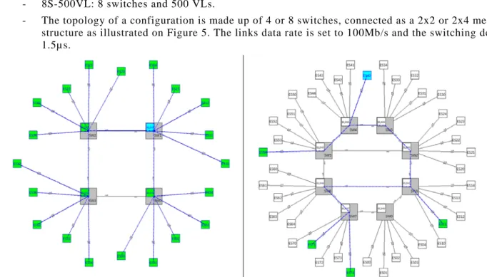
- 8S-200VL: 8 switches and 200 VLs, - 8S-500VL: 8 switches and 500 VLs.
- The topology of a configuration is made up of 4 or 8 switches, connected as a 2x2 or 2x4 mesh structure as illustrated on Figure 5. The links data rate is set to 100Mb/s and the switching delay to 1.5µs.
Figure 5: Topology of the case studies. The right-hand figure shows the 4 switches 2x2 mesh topology configuration with a synchronization frame broadcasted by switch 1. The left-hand figure shows the 8-switches 2x4 network configuration with a multicast stream (RTaW-Pegase screenshots).
Five end-systems are connected to each switch. Then, the predefined number of VLs is created with the following procedure for each VL:
- The number of receivers is randomly chosen between 1 and 5 with a uniform distribution, and the destination nodes are randomly selected (avoiding the source). The expected total number of flows is hence 3 times larger than the number of VLs.
- The size of the frames of the VL is randomly chosen according to a uniform distribution: as many more small frames, but still some large ones. The range of the size distribution is adjusted wrt the network load objective and the number of VLs.
- The frame rate, or BAG, is randomly chosen with a uniform distribution in the set of values authorized by the AFDX standards. The BAG value is biased towards large values. Indeed, with an equiprobable choice, the load generated by larger BAG value flows (e.g., 128ms BAG) would have been negligible compared to the load of the smaller BAG flows (e.g., 2ms BAG).
2 . 3 D i s t r i b u t i o n s o f B A G a n d f r a m e s i z e
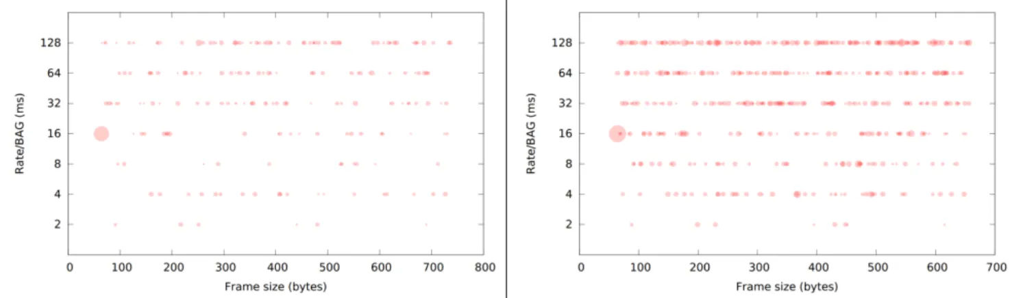
The distributions resulting from the random generation for the BAG and frame size of the VLs is shown in Figure 6 for the 4S-200VL configuration, where the area of the circles is proportional to the number of VLs with these parameter values. For example, the top-left circle shows that there is only one VL with BAG 128ms and maximal size 107bytes, and the large circle near the 16 label shows that they are 29 VLs with BAG 16ms and size 64 bytes.
Figure 6: Distribution of BAG and frame size for the 4S-200VL configuration.
The load on the links between the switches in the 4S-200VL configuration ranges from 2.05% to 7.56%, the variability being due to the randomness of the configurations. The same distributions are shown for the 8-switches 200 VLs configuration (8S-200VL) and the 8-8-switches 500VLs configurations in Figure 7. For these two latter configurations, the load of the links between the switches respectively ranges from 3.31% to 16.68% and from 5.20% to 27.45%. The larger load in these configurations is due to the larger number of VLs but also to the larger maximum frame size (twice the maximum size used to generate the first configuration).
2 . 4 E x p e r i m e n t s : i n c r e a s i n g T T t r a f f i c w i t h / w i t h o u t s c h e d u l e r e g e n e r a t i o n
The aim of this study is to evaluate the impact of the TT traffic over the RC traffic. This will be assessed by gradually increasing the share of the TT traffic while simultaneously reducing the RC traffic by the same amount. This comes to consider networks where an increasing share of the RC traffic is turned into TT traffic. At each stage, the WCTTs of the RC flows are recomputed.
We first consider a configuration entirely consisting of RC traffic, called “0 TT”. We then split this configuration into 10 subsets of VLs (S1, S2, S3,…, S10) , each subset being made up of 10% of the VLs:
- The VLs in S1 are transformed into TT traffic, the rest of the traffic remaining RC. This configuration is denoted by “S1 TT”.
- On the basis of “S1 TT”, S2 is turned into TT traffic. This configuration is denoted by “S1-2 TT”. - This goes on until one ends up with a complete TT configuration (“S1-10 TT”), leading overall to
11 configurations.
The frames of all TT flows are assumed to have a deadline constraint equal to the period of the flow. For each traffic configuration under study, two different experiments are performed:
- Experiments A: a global schedule is built for the TT flows, the routing is set for all flows of the 11
configurations, and an upper bound on the WCTTs of the RC flows is computed. From the scheduling point of view, each configuration is a new problem submitted to the off-line scheduler TTE-Plan, and there is no link between two flow configurations. In particular, the scheduler will often choose different routes for the same VL in the RC class, as it will be seen later in the experiments.
- Experiment B: we start with “S1-S10 TT” where all flows are in the TT class. A global TT
schedule is built for this configuration. Then, 10%, 20% and up to 100% of the flows are progressively becoming RC, but the same schedule is kept for the remaining TT flows, and the routing remains the same as in is “S1-S10 TT” for all VLs.
Keeping the same routing and same TT schedule as done in experiment B eases the comparisons but this is not optimal in terms of scheduling performances. Indeed, our observation has been that the off-line TT scheduler tries to spread the TT slots as uniformly as possible over time, creating hence time windows for the RC frames to be transmitted with little delays, and subtracting TT slots at random will not lead to an optimally balanced TT load.
3 P e r f o r m a n c e s o f m i x e d T T a n d R C c o n f i g u r a t i o n s – a n e m p i r i c a l
e v a l u a t i o n
The performance evaluation study is conducted by progressively turning RC VLs into TT VLs and studying the impact on the RC flow latencies. The outcomes of the experiments are difficult to predict because there are different and conflicting effects of the TT traffic over the RC traffic:
1. Priority change: in AS6802, the TT flows have a higher priority than the RC flow. Hence, moving a flow from RC to TT will reduce the remaining bandwidth left to the RC flows, and increase their delays.
2. Loss of bandwidth: When the integration method is timely block, some bandwidth just before a TT window may have to be left unused, increasing thus the delays of the RC traffic.
3. Contention reduction: The TT frames are scheduled by the off-line scheduler TTE-Plan which will shape the TT traffic over time. Indeed, the scheduler tries to spreadthe TT time-windows along the system hyper-period. This is beneficial for RC flows since it reduces the number of frames and thus the waiting times in the communication switch queues.
To illustrate contention reduction, let us consider the topology in Figure 1 assuming that all flows are converging to station R2. The flows F1 and F2 are TT while the flow F3 is RC, and all flows have the same BAG. By shaping the TT load along the hyper-period, the scheduler will insert idle times between the time windows of both TT flows. Hence, the RC frame from flow F3 can be delayed either by a frame of F1 or a frame of F2 but not by both, as illustrated in Figure 8. On the contrary, if the flows F1 and F2 were RC, they could arrive at the switch back-to-back and the RC flow would be delayed by both.
Figure 8: TT shaping reduces contention by idle times by TT time windows. 3 . 1 C o n f i g u r a t i o n w i t h 4 s w i t c h e s a n d 2 0 0 V L s ( 4 S - 2 0 0 V L )
The graphs on Figure 9 show the worst-case traversal times (WCTT) of the RC flows with shuffling and timely block in Experiments A (communication schedule regeneration at each step). It must be noted that The outliers are due to flows whose routing was changed with respect to their routing in their 0TT configuration. Indeed, the changes of routing negatively impact many RC flows. We observe anyway that globally an increasing share of TT traffic helps to reduce the RC WCTTs (see also Table 1). This holds for both shuffling and timely block. Here, the positive shaping effect outweighs the detrimental effects listed previously as soon as the TT load is above 20%.
Figure 9 : Upper bounds on the worst-case traversal times (WCTT in ms) for the rate-constrained flows in Experiments A on the 4S-200VL configuration with shuffling (left) and timely block (right). The curves show the WCTTs for a share of TT traffic equal to 0% (0TT), 20% (20TT), 50% (50TT) and 70% (70TT). The VLs are sorted by increasing WCTTs in the 0TT configuration.
As can be seen in Figure 10 that shows Experiments B (i.e., no TT schedule regeneration at each step), shuffling is logically better (12.5% on average over all flows) for RC flows than the timely block scheme. In experiments B with shuffling (see Table 1), the average WCTT for RC flows is 1.20ms with 0% TT load, 1.08ms with 20% TT load, 0.82ms with 50%TT load and 0.33ms with 90% TT load. However, this large latency improvement, up to 72% over purely RC traffic, is only for the reduced set of RC flows left.
Figure 10 : Upper bounds on the worst-case traversal times (WCTT in ms) for the rate-constrained flows in Experiments B on the 4S-200VL configuration with shuffling (left) and timely block (right) for an increasing share of TT traffic (0 to 70%).
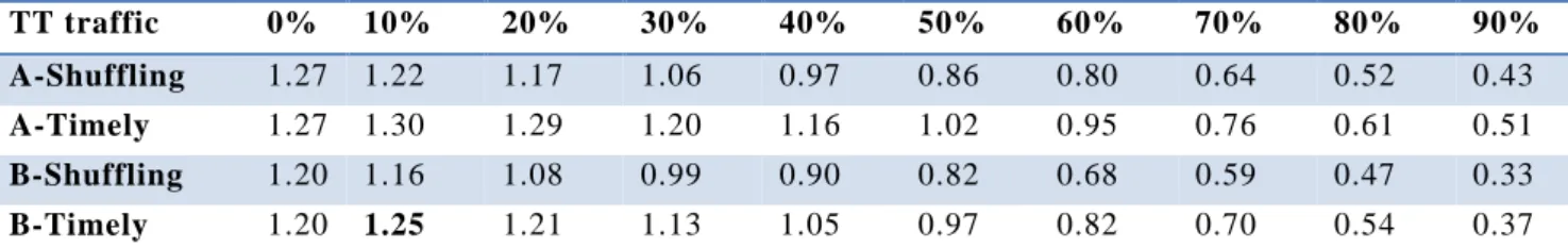
Table 1 summarizes the results over all traffic configurations for Experiments A and B. The small difference there is at 0% TT load can be explained by differences in the routing provided by TTE-Plan. On this small system, except in one case, the WCTTs of RC flows decrease monotonously with the increase of
the TT traffic. The number in bold in Table 1 shows a case where the loss of bandwidth due to timely block is not fully compensated by the better shaping of the TT traffic.
TT traffic 0% 10% 20% 30% 40% 50% 60% 70% 80% 90% A-Shuffling 1.27 1.22 1.17 1.06 0.97 0.86 0.80 0.64 0.52 0.43
A-Timely 1.27 1.30 1.29 1.20 1.16 1.02 0.95 0.76 0.61 0.51
B-Shuffling 1.20 1.16 1.08 0.99 0.90 0.82 0.68 0.59 0.47 0.33
B-Timely 1.20 1.25 1.21 1.13 1.05 0.97 0.82 0.70 0.54 0.37
Table 1: Average WCTT in ms of RC flows with an increasing share of TT traffic on the 4S-200VL configuration. ‘A-Shuffling’ stands for experiments A with shuffling traffic integration mechanism.
Due to space constraints, the results are not shown in this paper for the configuration with 8 switches and 200VLs. The reader is referred to [Bo15] for the complete set of experimental results.
3 . 2 C o n f i g u r a t i o n w i t h 8 s w i t c h e s a n d 5 0 0 V L s ( 8 S - 5 0 0 V L )
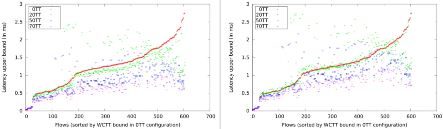
In this section the same experiments are conducted on a larger configuration in terms of topology (number of switches and stations). The frame size is also twice the size used for the smaller system. As a result of that, the network is more highly loaded with links loads up to 27.5% (see §2.3). Figure 11 shows the WCTTs for the RC traffic with timely block on experiments A (left graphic) and B (right graphic). WCTTs obtained with Experiments A form a cloud of points in the left-hand graphic of Figure 7 because, in this more constrained problem, the off-line scheduler defines for the majority of RC flows different routes at the different TT load levels. The gain obtained with TT traffic can best be seen in Figure 12 (left graphic). However, as seen on Figure 11 (right graphic) and Figure 12 (right graphic), on the contrary to the results obtained with the small system, here more TT load leads to degraded performances for the RC traffic when timely block is used. Indeed this mechanism involves a loss of bandwidth for RC frames that increases with the number of TT frames exchanged in the system.
Figure 11 : Upper bounds on the worst-case traversal times (WCTT in ms) for the rate-constrained flows in Experiments A and Experiments B on the 8S-500VL configuration with timely block (right) for an increasing share of TT traffic (0 to 70%).
Figure 12 : Upper bounds on the worst-case traversal times (WCTT in ms) for the rate-constrained flows in Experiments B on the 8S-500VL configuration with shuffling (left) and timely block (right) for an increasing share of TT traffic (0 to 70%).
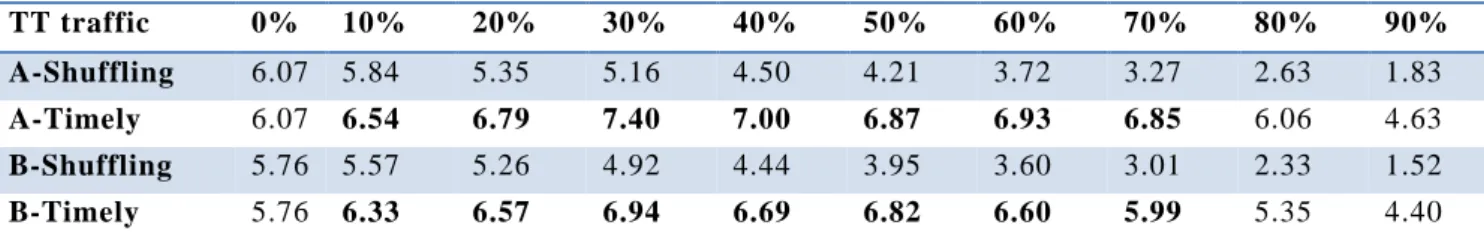
What we see in Table 2 is that on this more loaded configuration shuffling clearly outperformed timely block for RC traffic WCTTs. In both Experiments A and B, the WCTTs of RC flows steadily decrease with an increasing share of TT traffic with shuffling, while, with timely block, RC flows have larger latencies with TT traffic up to 80% of TT traffic. The larger the TT load, the higher the performance difference between shuffling and timely block. Indeed, the average WCTT response times of RC frames are more than 2 times larger with timely block above 50% of TT traffic in Experiments A and B.
TT traffic 0% 10% 20% 30% 40% 50% 60% 70% 80% 90% A-Shuffling 6.07 5.84 5.35 5.16 4.50 4.21 3.72 3.27 2.63 1.83
A-Timely 6.07 6.54 6.79 7.40 7.00 6.87 6.93 6.85 6.06 4.63
B-Shuffling 5.76 5.57 5.26 4.92 4.44 3.95 3.60 3.01 2.33 1.52
B-Timely 5.76 6.33 6.57 6.94 6.69 6.82 6.60 5.99 5.35 4.40
Table 2: Average WCTT in ms of RC flows with an increasing share of TT traffic on the 8S-500VL configuration. ‘A-Shuffling’ stands for experiments A with shuffling traffic integration mechanism.
In our experiments on the large configuration with 8 switches and 1500 flows, we observed that, when using timely-block, scheduling a share of the flows as TT traffic could degrade the latencies of the RC flows. This degradation is however limited to 21% in our experiments. This same behavior could not be reproduced with shuffling which however leads to larger worst-case jitters for TT flows.
4 D i s c u s s i o n a n d f u t u r e w o r k
This study is to the best of our knowledge the first providing an evaluation of the impact of the TT traffic over the RC traffic in an AS6802 network mixing TT and RC traffic with different traffic integration policies. Experiments have been presented, which offer some insights about the interferences between both classes of traffic:
- The timely block integration has a detrimental impact on the RC traffic latencies with respect to shuffling, with an increase of more than a factor 2 over shuffling above 50% of TT flows.
- TT flows, as scheduled with TTE-Plan, tend to spread the network transmissions over time as a traffic shaping policy would do, which reduces the RC latencies. However this only holds with shuffling which incurs increased jitters for TT flows.
These results should however be interpreted with caution for the following reasons:
– The results obtained depend on the global TT schedule. The experiments presented here have been done using the Plan scheduler of TTTech. Another scheduler, or a modified version of TTE-Plan, may lead to different results. The performance of a Time-Triggered system depends on the ability to build an efficient global schedule; in others words, the performances of an AS6802 network depends not only on the network technology but also importantly on the configuration tool. – Other choices for the network configurations used in the experiments (probability distributions for
the random generation, assumption on the clock-drifts, topology choices, etc) may possibly have lead to different findings.
– We built with TTE-Plan a schedule considering only the shuffling integration method and used it also for timely block configuration. Our analyses on timely block are thus done using a schedule designed for the shuffling method.
– The algorithms computing the upper bounds on delays for RC frames only provides upper bounds, not the exact worst case which is unknown. There is currently no method to compute tight lower bounds on the worst-case delays, as it exists for AFDX [Ba09]. Hence there is no way to estimate the actual pessimism of our upper bound in a satisfactory manner. Although, experiences with previous similar analyses in Network Calculus (e.g. [Bo12]) suggest that the analysis should be accurate, this remains to be ascertained.
– At moderate load, the RC traffic benefits from the traffic shaping of the TT traffic, which is facilitated by the assumption that deadlines equal periods. On more constrained systems, with deadlines less than periods, it is possible that this beneficial effect will be less pronounced.
SAE6802, with its three classes of traffic, offers a lot of flexibility in terms of how the communication can be organized. It becomes however difficult for the system designer to know beforehand the impact of configuration choices on the communication latencies. This study is a step towards a better understanding
the behavior of SAE6802 and the influence of configuration parameters. Our aim is also to conceive and implement the toolset that will help automate the configuration and verification of SAE6802 networks. Given the number configuration choices parameters involved, we believe that design space exploration techniques that would guide the designer would help to raise the level of abstractions and lead to a faster and more secure design process. Ultimately, this work contributes to a better understanding of how to best integrate mixed-criticality traffic in complex networked embedded systems as currently investigated in the DREAMS FP7 EU project [Dr15].
Acknowledgments: This work has been partially funded by the FP7-ICT integrated project DREAMS
(FP7-ICT-2013.3.4-610640).
5 R e f e r e n c e s
[AS6802] “Time-Triggered Ethernet”, SAE standard AS6802, 2011.
[Ba09] H. Bauer, J.L. Scharbarg, C. Fraboul, Christian,”Applying and optimizing Trajectory approach for performance evaluation of AFDX avionics network”, 14th IEEE ETFA, Palma de Mallorca, 2009.
[Bo11] M. Boyer, J. Migge, M. Fumey, “PEGASE, A Robust and Efficient Tool for Worst Case Network Traversal Time“,SAE 2011 AeroTech Congress & Exhibition, Toulouse, France, 2011.
[Bo12] M. Boyer, N. Navet, M. Fumey (Thales Avionics), “Experimental assessment of timing verification techniques for AFDX“, Embedded Real-Time Software and Systems (ERTS 2012), Toulouse, France, 2012. [Bo14] M. Boyer, L. Santinelli, N. Navet, J. Migge, M. Fumey, “Integrating End-system Frame Scheduling for more Accurate AFDX Timing Analysis“, Embedded Real-Time Software and Systems (ERTS 2014), Toulouse, France, 2014.
[Bo14] M. Boyer, H. Daigmorte, N. Navet, J. Migge, “Performance impact of the interactions between time-triggered and rate-constrained transmissions in TTEthernet”, ONERA Technical Report, 2015.
[BD12] M. Boyer, D. Doose, “Combining network calculus and scheduling theory to improve delay bound”, 20th Int. Conf. on Real-Time and Network Systems (RTNS2012), 2012.
[DP15] D. Tamas–Selicean, P. Pop, W. Steiner “Timing analysis of rate constrained traffic for the TTEthernet communication protocol”, 18th IEEE Int. Symp. on Real-time Computing (ISORC), 2015. [DR15] Home page of the DREAMS (Distributed REal-time Architecture for Mixed Criticality Systems) FP7 EU project, http:// http://www.uni-siegen.de/dreams/home/, retrieved 13/11/2015.
[Fr06] F. Frances, C. Fraboul, J. Grieu, “Using Network Calculus to optimize AFDX network“, Proc. of the 3thd European congress on Embedded Real Time Software (ERTS06), 2006.
[Gr04] J. Grieu, "Analyse et évaluation de techniques de commutation Ethernet pour l’interconnexion des systèmes avioniques", Doctoral dissertation, Institut National Polytechnique de Toulouse, 2004.
[Gu13] JJ. Gutierrez, J.C. Palencia, M.G. Harbour, “Response time analysis in AFDX networks with sub-virtual links and prioritized switches” Proc of the XV Jornadas de Tiempo Real, Santander, Spain, 2012. [He12] E. Heidinger, N. Kammenhuber, A. Klein, G. Carle, “Network Calculus and mixed-integer LP applied to a switched aircraft cabin network”, Proc. of the IEEE 20th Int. Workshop on Quality of Service (IWQoS), 2012.
[Li11] X. Li, Xiaoting, J.L. Scharbarg C. Fraboul, F. Ridouard, ”Existing offset assignments are near optimal for an industrial AFDX network” Proc. 10th Int. Workshop on Real-tTme Networks (RTN 2011), Porto, Portugal, 2011.
[Na15] N. Navet, J. Seyler, J. Migge, "Timing verification of real-time automotive Ethernet networks: what can we expect from simulation?”, Presentation at the SAE World Congress 2015, "Safety-Critical Systems" Session, Detroit, USA, April 21-23, 2015.
[Se15] J. Seyler, T. Streichert, M. Glaß, N. Navet, J. Teich, “Formal Analysis of the Startup Delay of SOME/IP Service Discovery”, DATE 2015, Grenoble, France, March 9-13, 2015.
[Ste09] W. Steiner, G. Bauer, B. Hall, M. Paulitsch, and S. Varadarajan, “TTEthernet Dataflow Concept”, Proc. of Eighth IEEE International Symposium on Network Computing and Applications, 2009.
[St11] W. Steiner, “Synthesis of Static Communication Schedules for Mixed-Criticality Systems”, 1st IEEE Workshop on Architectures and Applications for Mixed-Criticality Systems (AMICS), 2011.
[Tam13] D. Tämas-Selicean, P. Pop, W. Steiner, “Synthesis of Communication Schedules for TTEthernet-Based Mixed-Criticality Systems”, 10th Int. Conf. on Hardware/Software Codesign and System Synt., 2013.