Effets des grands angles de zénith et de la couverture
nuageuse sur l’éclairement sous-marin: implications
pour la production primaire dans l'océan Arctique
Thèse
Srikanth Ayyala Somayajula
Doctorat interuniversitaire en océanographie
Philosophiæ doctor (Ph. D.)
Effects of large solar zenith angles and cloud cover
on underwater irradiance: Implications for
primary production in the Arctic Ocean
Thése
Srikanth Ayyala Somayajula
Sous la direction de :Marcel Babin, directeur de recherche Simon Bélanger, codirecteur de recherche
Résumé
Le processus de la photosynthèse nécessite l'énergie de la lumière solaire et, dans l’océan, se déroule essentiellement dans la couche euphotique. Outre les autres variables (à savoir la chlorophylle a et les paramètres photosynthétiques), une connaissance appropriée du champ lumineux en termes de rayonnement incident disponible sur la photosynthèse (PAR) à un emplacement, une profondeur et une heure et une date donnés, est requise par les modèles d'écosystème marin. Le travail inclus dans cette thèse examine comment des angles de zénith solaires plus grands et différentes conditions nuageuses caractéristiques des régions de haute latitude, en particulier dans l'Arctique, peuvent affecter la précision des estimations de l'éclairement de surface et dans la colonne d’eau. L’accent est également mis sur les variations du champs lumineux à haute fréquence liées à la nébulosité sur les estimations de la productivité primaire.
Les PAR de surface estimés à partir de différents modèles ont été comparés à des mesures en série chronologique in situ à haute fréquence de données de PAR d'une bouée située en mer Méditerranée. Nous avons examiné comment les incertitudes dues aux angles de zénith solaires plus grands, en conditions nuageuses variables, pouvaient affecter la précision des estimations de l'éclairement de surface. La méthode de classement objectif a été utilisée pour identifier les meilleures méthodes. Le produit PAR de la NASA-Ocean Biology Processing Group (OBPG) a montré les meilleures performances globales, tandis que les PAR basées sur la méthode de la table de conversion (LUT) ont présenté les meilleures performances en termes de différence carrée moyenne, de biais sous ciel clair et également par temps couvert. D'autres méthodes basées sur des formulations empiriques ont montré la troisième meilleure performance par temps clair, tandis que par temps nuageux, elles présentaient de plus grandes incertitudes. Trois méthodes testées par faible ensoleillement ont montré des incertitudes allant jusqu'à 50% dans toutes les conditions du ciel. Les
performances du modèle dépendent des propriétés et des produits de nuage.
Les estimations de la production primaire dans l’ensemble de la couche illuminée de l’océan exigent la connaissance du champ lumineux à n’importe quelle profondeur dans la colonne d’eau jusqu’à un niveau de rayonnement solaire minimal (c’est-à-dire la profondeur euphotique). La précision d'un modèle semi-analytique pour le coefficient d'atténuation diffuse verticale de l'éclairement de surface (!"#) dont les variables sont les propriétés optiques inhérentes de l’eau de mer (absorption et diffusion), et l’angle zénithal solaire, a été examiné pour des anges zénithaux solaires et une nébulosité élevés. Des simulations de transfert radiatif approfondies ont été effectuées pour quantifier les incertitudes dues aux grands angles zénithaux et aux nuages sur les estimations du coefficient d'atténuation diffuse. Les incertitudes dans ces deux conditions sont dues à la variabilité des proportions des parties directes et diffuses de l’éclairement total atteignant la surface et dans la colonne d’eau. En outre, un paramétrage amélioré du modèle a été proposé pour estimer !"# aux grands angles zénithaux et différentes conditions nuageuses. L'évaluation des résultats avec des données in situ de l'océan Arctique, à l'aide du paramétrage amélioré du modèle, a montré de bonnes performances avec une erreur relative de 17% par rapport aux 23% du paramétrage initial du modèle par temps clair.
La production primaire quotidienne intégrée en profondeur a été estimée à l'aide d'un modèle de photosynthèse-lumière pour différentes entrées de PAR, moyennées à différents pas de temps sur une journée (par exemple, 1h, 3h, 6h, etc.). Les mesures à haute fréquence de bouées caractérisant la variabilité diurne due aux angles zénithaux solaires et la variabilité due aux nuages sur l’éclairement en surface et le coefficient d'atténuation diffuse vertical, ainsi que des données de biomasse journalière par satellite et des paramètres de photosynthèse in situ à proximité d'une bouée permettent d'examiner l'incertitude dans les estimations de la production primaire en raison de la résolution temporelle. Des erreurs inférieures de 1,91% pour un ciel quasi dégagé, 2,74% pour un ciel partiellement dégagé et 3,58% pour un ciel couvert sont observées pour des entrées de PAR à 0,5h, 1h et 3h, alors que les erreurs varient de ~ 11% à 25,39% pour un ciel quasi claire à couvert avec des entrées de PAR moyennées sur 24h. Il a été observé que la précision des estimations de la production primaire dépendait des entrées de PAR de différentes résolutions temporelles et
de la couverture nuageuse. Enfin, l’impact de la résolution spatiale des PAR sur la production primaire a été quantifié à l’aide des données de télédétection couleur des océans. Les résultats de cette thèse montrent que la meilleure représentation des nuages et de leurs propriétés aux échelles spatiales et temporelles est importante dans les modèles pour améliorer la précision de l'estimation du PAR en surface. Les résultats suggèrent également que davantage d’efforts visant à mieux quantifier les incertitudes liées à la faible élévation du soleil doivent être consentis en multipliant les études d’évaluation dans différentes régions et à différentes échelles de temps. Les résultats soulignent également que les incertitudes dues aux nuages et aux grands angles zénithaux solaires dans la représentation du champ lumineux dans la colonne d'eau peuvent être améliorées. Un effort important en vue de considérer la représentation des mesures de cycle diurne avec des changements horaires des champs d’éclairement (dus aux nuages, par exemple) améliore les valeurs de PAR quotidiennes intégrées et donc les estimations de la production primaire. Il souligne donc que les futurs travaux de recherche et de modélisation visant à améliorer la compréhension de la production primaire océanique et de son rôle dans l’océan mondial devraient inclure un examen de la variabilité diurne des mesures d’éclairement dans la distribution de la production primaire.
Abstract
The process of photosynthesis requires the energy from sunlight and takes place essentially in the euphotic layer of the oceans. In addition to other variables (i.e., chlorophyll a and photosynthetic parameters) a suitable knowledge of light field in terms of photosynthetically available radiation (PAR) at any given location, depth and time is an important input parameter required by marine ecosystem models. The work included in this thesis examines how larger solar zenith angles, different cloud conditions that are characteristic features of high latitude regions, especially in Arctic, might affect the accuracy of surface irradiance estimates. Further, main focus was on the effects of high frequency variations in the light field on primary production.
Surface PAR estimated from different models were compared with high frequency in situ time series measurements of PAR a buoy located in Mediterranean Sea. It was examined how uncertainties due to larger solar zenith angles under varying cloud conditions might affect the accuracy of surface irradiance. Objective ranking method was used to identify the best methods. Methods tested under low sun elevations exhibited uncertainties as large as 50% under all sky conditions. Model performances were dependent on cloud properties and products.
Accuracy of a semianalytical model for coefficient of vertical diffuse attenuation of surface irradiance (!"#) based on optical properties inherent to the water itself (absorption and scattering), and solar zenith angle was examined under larger solar zenith angels and cloud conditions. Extensive radiative transfer simulations were performed to quantify the uncertainties due to large solar zenith angles and clouds on the estimates of diffuse attenuation coefficient. The uncertainties under both these conditions are due to the variability in the proportions of direct and diffuse parts of the total irradiance reaching the surface and in the water column. Also, an improved model parameterization proposed to estimate !"# under large solar zenith angels and cloud conditions was evaluated with Arctic
Depth integrated daily primary production was estimated using a photosynthesis-light model for various PAR inputs averaged at different time steps over a day (for ex. 1h, 3h, 6h etc.). High frequency measurements from buoy characterizing diurnal variability due to solar zenith angles and variability due to clouds on surface irradiance and vertical diffuse attenuation coefficient of irradiance along with satellite daily biomass data, and in situ photosynthetic parameters near a buoy location are used to examine the uncertainty in primary production estimates due to temporal resolution.
The results of this PhD work show that the better representation of clouds and their properties both on spatial and temporal scales are significant in the models to improve the accuracy in estimation of surface PAR. The results also suggest that more efforts to quantify uncertainties under low sun elevations by more evaluation studies in different regions and time scales are necessary in accurate estimation of PAR, which is important for primary production studies. Also, the results emphasize that the uncertainties due to clouds and at large solar zenith angles in representation of light field in water column can be improved. The representation of diurnal-cycle measurements with hourly changes in irradiance fields (e.g., due to clouds) improved the daily integrated PAR values and hence primary production estimates.
Contents
Résumé ... iii!
Abstract... vi!
Contents ...viii!
List of Tables ... xi!
List of Figures ...xiii!
List of Symbols ... xvii!
Acknowledgements ... xxi!
Foreword ... xxiii!
Introduction ... 24!
Chapter 1 - Evaluation of sea-surface photosynthetically available radiation algorithms under various sky conditions and solar elevations ... 42!
1.1 Résumé ... 42!
1.2 Abstract ... 44!
1.3 Introduction ... 45!
1.4 Materials and Methods ... 49!
1.4.1 The three radiative models ... 49!
1.4.1.1 NASA-OBPG (OBPG) ... 49!
1.4.1.2 Gregg and Carder (GC) ... 50!
1.4.1.3 Santa Barbara DIscrete Ordinate Radiative Transfer (DISORT) Atmospheric Radiative Transfer (SB) ... 51!
1.4.2 Cloud correction schemes ... 53!
1.4.2.1 Dobson and Smith cloud formulation (DS) ... 53!
1.4.2.2 Budyko (B) ... 53!
1.4.2.3 New cloud correction schemes (NC) ... 54!
1.4.3 Atmospheric parameters from remote sensing ... 54!
1.4.3.1 ISCCP dataset (IS) ... 54!
1.4.3.2 MODIS Atmospheric dataset (M) ... 55!
1.4.4 Definition of PAR Products... 56!
1.4.4.1 OBPG operational PAR product ... 56!
1.4.4.2 LUT method ... 56!
1.4.4.3 Clear sky models with CF corrections ... 57!
1.4.4.4 In situ PAR data for validation ... 57!
1.4.5 Statistical analysis and methods ranking ... 59!
1.5 Results ... 62!
1.5.1 Methods ranking and performance for daily and monthly PAR estimation ... 62!
1.5.2 Methods performance under quasi-clear sky, partly cloudy and overcast
conditions ... 65!
1.5.3 Spatial and temporal mismatch ... 70!
1.5.4 New cloud correction parameterization ... 73!
1.5.5 Instantaneous PAR estimation under low sun elevation ... 75!
1.6 Discussion... 79!
1.6.1 Performance of PAR estimation methods under all sky conditions, temporal and spatial mismatch ... 79!
1.6.2 Impact of clouds and cloud products on PAR estimation ... 81!
1.6.3 Impact of low sun elevations on PAR estimation ... 83!
1.6.4 Methods ranking ... 84!
1.7 Conclusions ... 85!
Chapter 2 - Performance of semianalytical algorithm for vertical diffuse attenuation coefficient of downwelling irradiance under large solar zenith angles and cloudy skies... 91!
2.1 Résumé ... 91!
2.2 Abstract ... 93!
2.3 Introduction ... 94!
2.4 Materials and Methods ... 95!
2.4.1 In situ measurements ... 95!
2.4.1.1 BOUSSOLE ($% − '()*) ... 96!
2.4.1.2 Ship-based observations of Rrs and $% in the Arctic ($% − +,-./-) ... 97!
2.4.2 AOP calculations ... 98!
2.4.3 $% modeling ... 98!
2.4.3.1 Forward modeling with Hydrolight ... 99!
2.4.3.2 Semianalytical model parameterization ... 100!
2.4.3.3 Inverse model for $% ($% − 011(3++)) ... 100!
2.4.4 Model performance assessment ... 101!
2.5 Results ... 102!
2.5.1 Evaluation of $% − 011 model performance with radiative transfer simulations ... 102!
2.5.2 Model performance with in situ Buoy and Arctic data ... 112!
2.6 Discussion... 119!
2.7 Conclusions ... 122!
Chapter 3 - Impact of high frequency surface irradiance measurements in a day on assessing primary production estimates ... 124!
3.1 Résumé ... 124!
3.2 Abstract ... 126!
3.4 Materials and methods ... 129!
3.4.1 Primary production model ... 129!
3.4.2 Photosynthetically available radiation (PAR) ... 130!
3.4.3 Vertical diffuse attenuation coefficient of downward irradiance ... 132!
3.4.4 Photosynthetic parameters ... 132! 3.4.5 Chlorophyll a ... 133! 3.4.6 Model performance ... 133! 3.5 Results ... 135! 3.6 Discussion... 143! 3.7 Conclusions ... 151! Conclusion ... 152! Bibliography ... 157!
List of Tables
Table 1. Description of PAR estimation methods from different sources and inputs under all sky conditions, the acronyms correspond to: OBGP: Ocean Biology Processing Group, SB: SBDART radiative transfer model, GC: Greg and Carder model, IS: ISCCP dataset, M: MODIS-Aqua dataset, DS: Dobson and Smith cloud attenuation formulation, B: Budyko cloud attenuation formulation as modified by Morel and Andre, NC: new cloud attenuation formulation (this study). ... 49! Table 2. Meteorological and sun variables represented in the Gregg and Carder (1990) model. ... 51! Table 3. Input parameters used in SBDART model to generate LUT ... 53! Table 4. Pearson’s Correlation Coefficient (r), RMSD (Ψ), CMRSD (∆), Bias (Ω), Slope (S) and Intercept (I) estimated between each method estimate and In situ for Daily and Monthly PAR values. RMSD, CMRSD and Bias are in units of mol photons m-2 d-1. The % values refer to relative RMSD and Bias. ... 67!
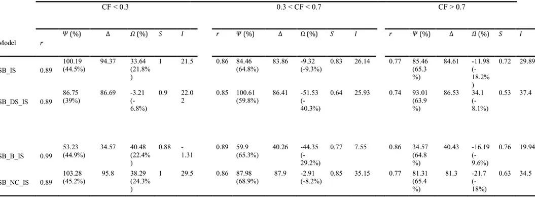
Table 5. Pearson’s Correlation Coefficient (r), RMSD (Ψ), CMRSD (∆), Bias (Ω), Slope (S) and Intercept (I) computed between each method estimate and in situ towards the study of impact of clouds and cloud products on PAR values under different sky conditions. RMSD, CMRSD and Bias are in units of in mol photons m-2 d-1. The % values refer to the relative RMSD and Bias. ... 69!
Table 6. Comparison of mean differences of daily integrated PAR modeled and estimated under different spatial and temporal binning for MODIS (1o ~ 77 km; 24 hr)
and ISCCP (2.5o ~ 280 km; 3 hr). The values are given in relative units. ... 71!
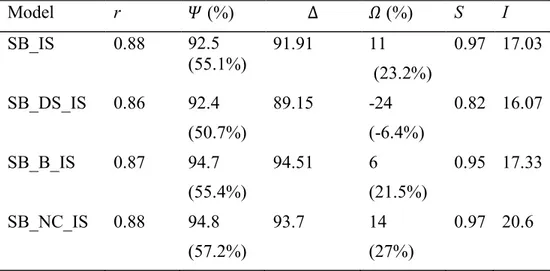
Table 7. Pearson’s Correlation Coefficient (r), RMSD (Ψ), CMRSD (∆), Bias (Ω), Slope (S) and Intercept (I) computed between each method estimate and in situ data under all sky conditions for low sun elevations. RMSD, CMRSD and Bias are in units of in µmol m-2 s-1. The % values refer to the relative RMSD and Bias.88!
Table 8. Pearson’s Correlation Coefficient (r), RMSD (Ψ), CMRSD (∆), Bias (Ω), Slope (S) and Intercept (I) computed between each method estimate and in situ data under different sky conditions for low sun elevations. RMSD, CMRSD and Bias are in units of in µmol photo m-2 s-1. The % values refer to the relative
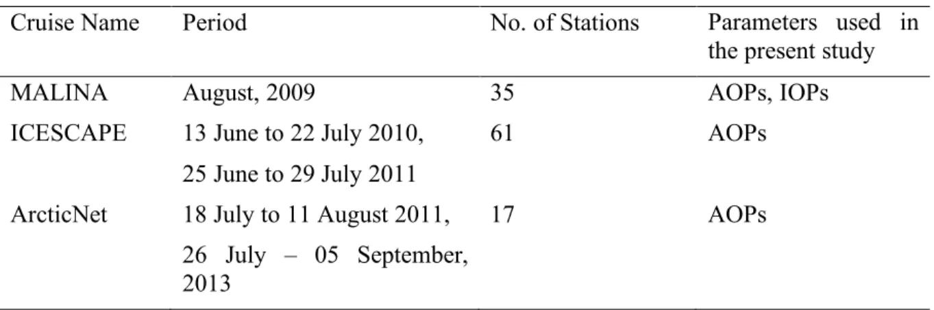
RMSD and Bias... 90! Table 9. In situ data used in the present study. ... 97! Table 10. Hydrolight model parameters for Sun at 70o, 75o, 80o, and 85o at depth ranges for
clear skies. ... 105! Table 11. Hydrolight model parameters for Sun at 30o, 60o, 70o, 75o, 80o, and 85o at depth
Table 12. Unique model parameters for Large solar zenith angles (LZA) at depth ranges for clear skies and for Sun at 30o, 60o, 70o, 75o, 80o, and 85o completely cloudy to
overcast skies. ... 111! Table 13. Comparison of !(d-Lee(QAA)) (0-10m) model with BOUSSOLE buoy in situ data at
09 m depth. ... 113! Table 14. Comparison of !(d-Lee(QAA)) (1) model with entire Arctic in situ data. ... 114!
Table 15. Comparison of !(d-Lee(QAA)) (E(10%)) model with ICESCAPE-2010&11 and Arctic
Net 2011&13 in situ data. ... 118! Table 16. Evaluation of new cloud parameterization for Kd (1) model with MALINA-2009
in situ data. ... 119! Table 17. Photosynthetic parameters at different depths used for the estimation of daily depth integrated primary production rates. ... 133! Table 18. RMSD and Bias of the daily depth integrated PP calculated with PAR(0+) data averaged over different time intervals, and under different photoinhibition (5) conditions. ... 135! Table 19. MAPE of the daily depth integrated PP modeled and estimated under different temporal binning using in situ data for different sky conditions. ... 139! Table 20. Comparison of MAPE between depth integrated PP estimated at 1 km and different spatial binning for MODIS-A for clear skies. ... 141! Table 21. Comparison of MAPE of daily depth integrated PP modeled and estimated under different spatial and temporal binning for MODIS (1o~ 77 km; 24 h) and ISCCP
List of Figures
Figure 1. The solar spectrum for direct light at both the top of Earth’s atmosphere and at sea level (https://commons.wikimedia.org/wiki/File:Solar_Spectrum.png,This figure was prepared by Robert A. Rohde as part of the Global Warming Art project. Permission is granted to copy, distribute and/or modify this document under the terms of the GNU Free Documentation License, Version 1.2 or any later version published by the Free Software Foundation; with no Invariant Sections, no Front-Cover Texts, and no Back-Cover Texts. A copy of the license is included in the section entitled GNU Free Documentation License). 26! Figure 2. Solar elevation above horizon during summer (a) or winter (b). Sun is seen during period L from sunrise (↑) till sunset (↓). ... 28! Figure 3. Example of clear-sky spectral downwelling plane irradiances Ed (λ) at the sea
surface for solar zenith angles of 30o and 60o (Ocean Optics Web Book • All
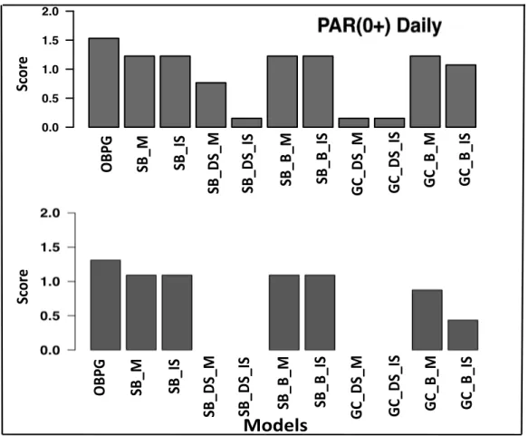
contents 2019 Creative Commons Attribution license. Permission is granted to copy, distribute and/or modify this document under the terms of the GNU Free Documentation License, Version 1.2 or any later version published by the Free Software Foundation; with no Invariant Sections, no Front-Cover Texts, and no Back-Cover Texts. A copy of the license is included in the section entitled GNU Free Documentation License). ... 31! Figure 4. Schematic representation of the optical properties of the water (cf. Mobley 1995, Ocean Optics Web Book • All contents 2019 Creative Commons Attribution license. Permission is granted to copy, distribute and/or modify this document under the terms of the GNU Free Documentation License, Version 1.2 or any later version published by the Free Software Foundation; with no Invariant Sections, no Front-Cover Texts, and no Back-Cover Texts. A copy of the license is included in the section entitled GNU Free Documentation License). 35! Figure 5. Photosynthesis-irradiance curve ... 37! Figure 6. Location of the BOUSSOLE site (black star). Background data corresponds to daily PAR for the month of June 2008, source MODIS L3 (Frouin et al. 1992 algorithm). ... 48! Figure 7. Top panel: score of the eleven models used to derive daily mean PAR(0+) (see table 4 for model details). Bottom panels: Modeled versus in situ PAR(0+) for the eleven models. The solid line corresponds to 1:1 line and the dashed-line corresponds to the linear fit of modeled versus in situ data. ... 63! Figure 8. Top panel: score of the eleven models used to derive monthly mean PAR(0+) (see table 4 for model details). Bottom panels: Modeled versus in situ PAR(0+) for the eleven models. The solid line corresponds to 1:1 line and the dashed-line corresponds to the linear fit of modeled versus in situ. ... 64!
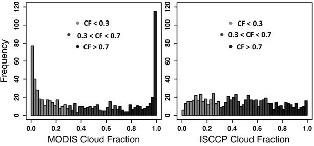
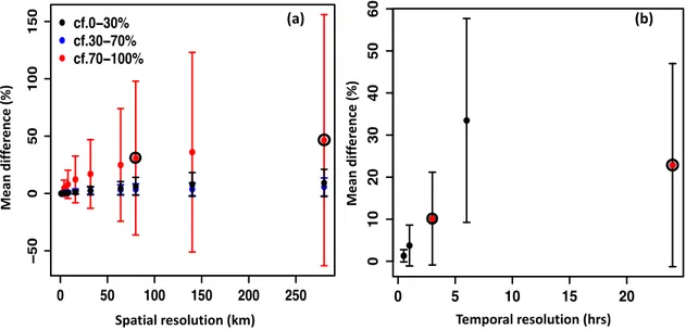
Figure 9. Scores of the selected models used to derive daily mean PAR(0+) under a) quasi-clear (CF<0.3), b) partially cloudy (0.3<CF<0.7) and c) overcast (CF>0.7)conditions (see table 5 for model details). d) d) Modeled versus in situ PAR(0+) for the selected models (see text for details). The solid line corresponds to the 1:1 line and the dashed-line corresponds to the linear fit of modeled versus in situ data. ... 68! Figure 10. Frequency distribution of a) MODIS and b) ISCCP daily mean CF values under quasi-clear (CF<0.3), partial (0.3<CF<0.7) and overcast (CF>0.7) cloud conditions. ... 70! Figure 11. (a) Mean percentage difference between daily PAR at 1-km resolution and PAR estimated 4-km, 8-km, 16-km, 32-km, 64-km, 80-km, 140-km and 280-km resolution for the year 2008 under varying sky conditions. The black circles correspond to MODIS (~ 77 km) and ISCCP (280 km) spatial resolutions. The black, blue and red vertical bars represent the lower and upper limits of the mean error for the three sky conditions (see text for details). (b) Mean percentage difference between daily-integrated PAR at 15 min time step and daily-integrated PAR at 30 min, 1 h, 3 h, 6h and 24 h time step for two months of BOUSSOLE buoy data under all sky conditions. The black circles correspond to ISCCP (3 hr binning) and MODIS (24 hr binning) temporal resolutions. The black vertical bars represent the lower and upper limits of the mean error. ... 71! Figure 12. a) Ratio PARcloud:PARclear as a function of CF for B (solid red line), DS ( solid
blue line) and the new cloud correction schemes (dashed line for ISCCP and dotted line for MODIS datasets). Ratio PARcloud:PARclear as a function of CF for
b) MODIS and c) ISCCP. The black solid line corresponds to the fitted relationships proposed in this study. Modeled versus in situ PAR(0+) for the new cloud-correction schemes for d) MODIS and e) ISCCP products. The solid lines in d) and e) corresponds to 1:1 line and the dashed-line corresponds to the linear fit of modeled versus in situ data. ... 74! Figure 13. Modeled versus in situ instantaneous PAR(0+) for the four methods (see table 7 for model details). The solid line corresponds to the 1:1 line and the dashed-line corresponds to the linear regression of modeled data versus in situ data. ... 75! Figure 14. Modeled versus in situ instantaneous PAR(0+) for SB_IS, SB_DS_IS, SB_B_IS and SB_NC_IS under a) quasi-clear (CF<0.3), b) partially cloudy (0.3<CF<0.7) and c) overcast (CF>0.7) conditions (see Table 8 for details). The solid line corresponds to the 1: 1 line and the dashed-line corresponds to the linear fit of modeled versus in situ data. ... 77! Figure 15. Normalized residuals of the four methods (see table 1.7 for model details) as a function of a) ISCCP τcl, b) ISCCP CF and c) θ0. Vertical dashed line in c)
corresponds to sun zenith angle of 78.5o and the solid black line corresponds to
a percentage residual equal to zero. ... 78! Figure 16. Methods scores with (top) and without (bottom) the inclusion of SB_DS_M, SB_DS_IS, GC_DS_M and GC_DS_IS methods. ... 84!
Figure 17. A map depicting sampling locations for the MALINA, ICESCAPE, ArcticNet cruises in Arctic and BOUSSOLE buoy site in the Mediterranean Sea. ... 97! Figure 18. Comparison of $% − 011 (1) and Hydrolight simulated $% − 60 − 07+ − -819,(1) for sun for 70o, 75o, 80o, and 85o under clear sky conditions. ... 103!
Figure 19. Comparison of (a) !: − ;<<(Ed10%) and (b) !: − ;=>(Ed10%) with
Hydrolight simulated Kd-HL-LZA-clear(Ed10%) for 70o, 75o, 80o, and 85o under
clear sky conditions. ... 103! Figure 20. Comparison of !: − ;<< (1) (a, b, c, & d) and !: − ?@AB: (1) (e, f, g, & h) with Hydrolight simulated !: − C; − D@AB:(1) for sun at 30o, 60o 75o, and 85o
under different cloudy sky conditions. Note that results for 70o and 80o are
similar to 75o and 85o, hence only results at 75o and 85o are presented here for
the cloud cover cases. ... 106! Figure 21. Same as Figure 20, but for !: − ?@AB:(Ed10%). ... 107!
Figure 22. Hydrolight simulations of !:(1) and !:(Ed10%) models for varying sun
geometry, cloud amount and absorption coefficient. ... 109! Figure 23. Same as Fig. 22, but for three ratios of backscattering to absorption (bb/a) coefficients. ... 110! Figure 24. Comparison of !: − ;<<(QAA)(0-10m) with !: − EBAF(0-9m) from time series at 9 m water column depth for sun at 30o, 60o, 70o and 80o under all sky
conditions. ... 112! Figure 25. Solar zenith angle dependency of !(d-buoy)(0-9m)... 114!
Figure 26. Comparison of !: − ;<<(G>>)(1) with !: − >HDIJD(1) in Arctic ocean during MALINA-2009, ICESCAPE-2010&11 and Arctic Net-2011&13 for 412, 443, 490, 510 ,555 nm and at all wavelengths. ... 116! Figure 27. Comparison of !: − ;<<(G>>)(Ed10%) with !: − >HDIJD(Ed10%) in Arctic
ocean during ICESCAPE-2010&11 and Arctic Net-2011&13 for 412, 443, 490, 510 ,555 nm and at all wavelengths. ... 117! Figure 28. Comparison of !: − ;<<(1) obtained from QAA, and !: − D@AB:(1) model parameters using MALINA cruise data with !: − >HDIJD(1) in Arctic Ocean at all wavelengths. ... 118! Figure 29. Distribution of relative error (%) as a function of absorption, solar zenith angles (x-axis) and cloud amount (different panels) between Hydrolight simulated !:(1) values against !: − ;<<(1) estimates (red dashed line shows the average relative under all absorption conditions). ... 120! Figure 30. Distribution of relative error (%) as a function of total absorption at different wavelengths between QAA derived values against in vivo measurements. .... 121! Figure 31. Locations of the BOUSSOLE (red dot) buoy and PROSOPE (green dot) cruise in the Mediterranean Sea. ... 131! Figure 32. Scatter plots for comparison of daily depth PP estimates obtained with PAR(0+)
calculated with PAR(0+) data at 0.25 time intervals. The black, red and green
symbols represent 5 = 0, 0.01 and 0.1 mg C. (mg Chl)-1 h-1.(Kmol photons m-2
s-1)-1 (the axis is on log scale). ... 135!
Figure 33. Mean absolute percentage error between daily PP estimates obtained with PAR(0+) averaged over 0.5, 1, 3, 6, 12 and 24h time intervals as function of PP calculated with PAR(0+) data at 0.25h time intervals. The black, red and green vertical bars represent the lower and upper limits of the mean error for beta = 0, 0.01 and 0.1. The dashed lines represent the error levels of 3%, 10% and 18% respectively from bottom to top. ... 137! Figure 34. Mean absolute percentage error between daily PP estimates with PP15min and PP
at 0.5h, 1h, 3h, 6h, 12h and 24h integrated daily PAR inputs to the P-I model. The black vertical bars represent the lower and upper limits of the mean error for different sky conditions. The dashed lines represent the error levels of 10%, 20% and 25% respectively from bottom to top. ... 138! Figure 35. MAPE between daily PP estimates with PAR(0+)1km and PAR(0+) at 4 km,
8km, 16km, 32km, 64km, 80km, 140km and 280km spatial PAR inputs to the P-I model. The black, red and green vertical bars represent the lower and upper limits of the mean error for beta =0, 0.01 and 0.1. ... 141! Figure 36. PAR distribution curve and the corresponding PAR(0+) daily values (in mol photons m-2 d-1) obtained over different time integration steps for curves given
a-g) a cloud less day, h-n) during the presence of intermittent clouds. ... 143! Figure 37. PAR(0+) daily time profiles during varying sky conditions (the red dot indicates
the noon value used to model 24h daily PAR estimate). ... 145! Figure 38. PAR(0+) daily time profiles obtained based on daily noon value (bell-shaped
profile represented by black circles) and profile from in situ measurements (light blue dotted line). Red dot indicated the local noon value. PAR24h and
PARref gives the PAR(0+) daily values obtained from the two profiles
respectively. ... 146! Figure 39. Daily PAR profiles (bell-shaped profile indicated by black circles) obtained based on instantaneous noon value. Red dot represents the noon value from in situ measurements. PARnoon values is given in µmol photons m-2 s-1, PAR24h
and PARref gives the PAR(0+) daily values obtained from the bell-shaped
profile and the measured values respectively, PPref and PP24h represents the PP
estimates from PAR24h and PARref inputs... 148!
Figure 40. Distribution of PAR(0+) values (blue dotted line), cloud fraction value for
ISCCP (brown dots at 3h time interval) and MODIS (green dot at 13:30 pass) for a given day... 150!
List of Symbols
Symbol Definition Units
a absorption coefficient m-1
b scattering coefficient m-1
bb backscattering coefficient m-1
Lw water leaving radiance W m-2 nm-1 sr-1
Lu upwelling radiance W m-2 nm-1 sr-1
Ed(z) downwelling irradiance at depth z W m-2 nm-1
EM(0O) Downwelling surface irradiance Kmol photons m-2 s-1
Es above surface irradiance W m-2 nm-1
Rrs remote sensing reflectance (ratio of water-leaving
radiance to downwelling irradiance above the surface)
sr-1
Kd diffuse attenuation coefficient for downwelling
irradiance m
-1
!"#(P) diffuse attenuation coefficient for downwelling irradiance between 0 m and depth z
m-1
!"#(QRS%) diffuse attenuation coefficient for downwelling irradiance between EM(0) m and 10% of EM(0)
m-1
KMVWX Downward diffuse attenuation coefficient for the PAR m-1
PAR(z, t) Photosynthetically available radiation at a given depth z
(m) and time Kmol photons m
-2 s-1
θS above surface sun zenith angles degrees
P` Normalized production to chlorophyll a biomass mg C (mg Chl a)-1 h-1
Pa` Maximum production rate at light saturation mg C (mg Chl a)-1 h-1
b Initial slope of the P-I curve mg C (mg Chl a)-1 h-1.(cK
mol photons m-2 s-1)-1
β Negative slope of the P-I curve at high light levels mg C (mg Chl a)-1 h-1.(cK
mol photons m-2 s-1)-1
Chlca Chlorophyll a concentration mg m-3
LUT Look-up Table CF Cloud Fraction
Dedicated to the Lotus feet of SRI SITA RAMA and to Dhana Lakshmi and Raga Amruta
Acknowledgements
First of all, I would like to thank my supervisor, Marcel Babin for giving me the opportunity to work in marine optical and primary production studies. Thank you for being a never-ending source of inspiration in the scientific work and your way of handling the tasks. I am very thankful for your support throughout the project, which make the research possible and giving me the opportunity to be a part of Takuvik research group. I also want to thank my co-supervisor Simon Bélanger for his insightful discussions on modelling aspects and related science. His expertise on marine light field and its processes was significant for this study. My sincere thanks to my committee member Warwick Vincent, for his inspirational talks during my course work, also Jean-Éric Tremblay for their constructive, appreciated advice on my work during committee meetings.
Next, I would like to thank Emmanuel Devred for always being there for me. I really enjoyed working together with you and found our discussion fruitful and inspiring. I thank you for your patience in my process of learning R programming and for making me to realize the amazing things it does. I have learnt a lot from you and appreciate that have made me feel that my work is really important. I want to thank Eric Rehm for discussions on Hydrolight simulations. Thanks to Atsushi Matsuoka who gave me advice during my initial PhD work. I am grateful to Maxime Benoit-Gagné, Guislain Bécu, and Phillippe Massicotte for programming assistance. I thank Flavienne Bruyant for her help with discussions on photosynthetic parameters. I thank David Antoine and Vincenzo Vellucci for their help with BOUSSOLE data and in manuscript preparation.
Thanks to all my colleagues who helped me during my PhD time at Takuvik lab for their dicussions: Sophie Renaut, Moritz Schimid, Deo Florence Onda, Jordon Grigor, Julien Laliberté, Nicolar Schiffrine, Marti Gali Tapais. My sincere thanks to Marie-Hélène Forget and Debra Christiansen Stowe for the invaluable moral support during my initial days in Québec City.
Canada’s New Arctic Frontier for a postgraduate scholarship, and to Québec-Océan for stipends made this project possible. Thanks to Canadian Space Agency funding support. I am very grateful to my brother Praveen and his family for their support during the last days of my PhD completion.
Finally, words fail to express the appreciation I have for my beloved wife Dhana Lakshmi and our daughter Raga Amruta’s support. She encouraged me to follow my dreams and take this path and ways my foundation throughout. She has my utmost respect and admiration, and of course, my deepest love. You have always respected my work and done everything possible to give me as much time as I needed to finish up this PhD work by taking good care of our loving daughter Raga Amruta.
Foreword
This doctoral thesis comprises a general introduction, three scientific articles (Chapters 1, 2 and 3), and general conclusions. Chapter 1 published in Applied Optics. Chapters 2 and 3 are in preparation for publication:
Chapter 1
Srikanth Ayyala Somayajula, Emmanuel Devred, Simon Bélanger, David Antoine, V.
Vellucci, and Marcel Babin, (2018), "Evaluation of sea-surface photosynthetically available radiation algorithms under various sky conditions and solar elevations," Appl. Opt. 57, 3088-3105.
(reproduced with permission of the publisher) Chapter 2
Srikanth Ayyala Somayajula, Emmanuel Devred, Simon Bélanger, David Antoine, V.
Vellucci, and Marcel Babin, Performance of semianalytical algorithm for vertical diffuse attenuation coefficient of downwelling irradiance under large solar zenith angles and cloudy skies.
Chapter 3
Srikanth Ayyala Somayajula, Marcel Babin Impact of high frequency surface irradiance
measurements in a day on assessing primary production estimates.
Introduction
Background
In Arctic Ocean, the consequences of increasing temperatures due to climate change results in drastic decrease in summer sea ice cover (Chapman and Walsh, 1993; Grebmeier et al.) and predicted that by the end of the current century the summer sea ice cover will completely disappear (Serreze et al. 2007). This increase in the length of ice melt season (Smith, 1998; Rigor et al. 2002; Serreze et al. 2007; Camiso et al. 2008) results in a positive feedback loop (refer to as the albedo feedback) in which greater open water area increased absorption of solar radiation by seawater and subsequent increase in sea surface temperature that further melts sea ice (Perovich et al. 2007). Moreover, changing ice cover and increase in melt pond fraction on sea ice amplifies the light transmission through sea ice and increase the light availability, which is the primary energy source for primary productivity (Arrigo et al. 2008a, 2012; Nicolaus et al. 2012; Popova et al. 2010). Also, light transmission through the melt ponds on sea ice triggers the development of underwater phytoplankton blooms (Arrigo et al. 2012) and ice-edge blooms are the main mode of productivity in the pan-Arctic region (Perrette et al. 2011). Light availability as determined by solar angle, ice thickness and, snow cover are one of the major forcing mechanisms that control annual Arctic Ocean primary productivity (Sakshaug, 1989; Wassman and Reigstad 2011). The Atmospheric light incident in the Arctic Ocean is characteristic of prevailing higher sun zenith angles (low sun elevations) that impact the magnitude of direct and diffuse light at the sea surface and the persistent clouds induces high-frequency fluctuations. Existing ocean color primary productivity models (Saba et al. 2011) that are recently implemented in the Arctic Ocean (Lee et al. 2015), must be improved towards how light availability for photosynthesis is affected under such a regime. It is evident that there is an increase in phytoplankton productivity in the Arctic under prevalent irradiance fluctuations due to an increase in cloud cover (Bélanger et al. 2013). Thus, further investigation is necessary on the variability of surface solar irradiance under prevailing high solar zenith angles, and clouds in terms of downwelling irradiance (Q#),
diffuse attenuation coefficient for downwelling irradiance (!#), and photosynthetically active radiation (PAR) to significantly improve our understanding of and ability to model primary productivity in the Arctic region.
Solar radiation
Solar radiation plays a significant role in driving the physical circulation of the atmosphere, the oceans, and the biological processes responsible for life sustainment on Earth. However, the amount of that radiation reaching the Earth varies depending on the location, season, atmospheric light absorption and reflection due to gases and aerosols, including clouds (Gill, 1982; IPCC, 2007). At the top of the atmosphere, the distribution of electromagnetic radiation emitted by the Sun is called solar spectrum. Of the electromagnetic energy emitted from the Sun, approximately 50% lies in the wavelengths longer than the visible region, about 40% in the visible region (400-700 nm) and about 10% in wavelengths shorter than the visible region (Liou, 1980). At the distance of the Earth’s orbit (150 x 106 km) the solar flux per unit area facing the Sun is about 1373 Wm-2
(Johnson, 1954). This quantity, the total solar irradiance outside the Earth’s atmosphere, is sometimes called solar constant. The spectrum at the mean Sun-Earth distance of 1 astronomical unit (AU), is used to calculate the extraterrestrial spectrum at the top of the Earth’s atmosphere (Fig. 1).
Several atmospheric factors modify the solar irradiance between the top of the atmosphere (TOA) and the Earth’s surface. All of them have differing transmittance with wavelength, and with the density of the atmospheric constituents themselves.
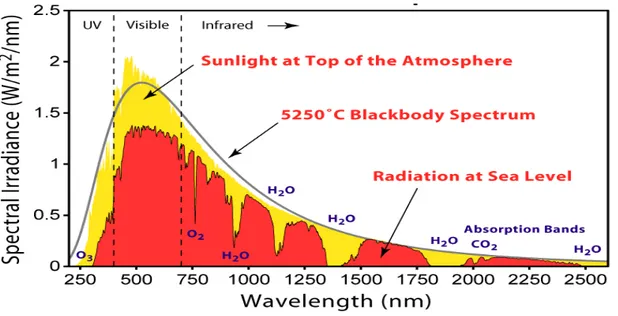
Figure 1. The solar spectrum for direct light at both the top of Earth’s atmosphere and at sea level (https://commons.wikimedia.org/wiki/File:Solar_Spectrum.png,This figure was prepared by Robert A. Rohde as part of the Global Warming Art project. Permission is granted to copy, distribute and/or modify this document under the terms of the GNU Free Documentation License, Version 1.2 or any later version published by the Free Software Foundation; with no Invariant Sections, no Front-Cover Texts, and no Back-Cover Texts. A copy of the license is included in the section entitled GNU Free Documentation License).
The spectral range from 400 to 700 nm is called photosynthetically available radiation (PAR) and is a critical parameter for plant photosynthesis. PAR is expressed in two types of units, i) it is defined as the radiometric flux per unit area and is expressed as Watts per square meter (W m-2). If E
M(i) is the downward spectral irradiance at wavelength i, then
PAR in W m-2 is expressed by the equation (Frouin and Pinker, 1995):
PARc(Wcmlm) = ∫ E
M(i)c:i pSScqa
rSScqa (1)
ii) in another unit, it is defined as the number of photons incident per unit area per unit time and is expressed in micromoles per square meter per second (Kmol m-2 s-1) expressed by
equation b:
PARc(scmolcmlmcslR) = R
ℏw∫ λcEM(i)c:i pSScqa
Where ℏ is Plank’s constant and c is the velocity of light in vacuum.
PAR traversing from the top of the atmosphere (TOA) to the Earth’s surface gets modified by the atmospheric composition. Thus, changes in the atmospheric composition with time plays an important role in the amount of PAR incident at the Earth’s surface. Several physical and statistical models can accurately estimate the PAR at the Earth’s surface under a clear sky (e.g. model 6S: Vermote et al., 1995, 1997a, 1997b).
Diurnal changes
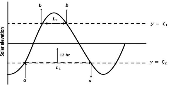
Diurnal changes of solar radiation reaching the surface follow a complex pattern. The main variability in irradiance is a function of solar elevation (Monteith, 1973). For a given day, at the equator the sun height, h, may be given by:
ℎ = ℎz{|sin 2ÄcÇÅ (3)
where h = tangent of angle which the sun makes with the horizon; hmax = maximum value of h;
É = day length (12 h);
t = É in fractions, starting at t = 0cÉ at sunrise, t = 1/4cÉ at noon, t = 1/2cÉ at sunset. Depending on season and geographical position the sun is seen for a shorter or longer period than half the sine curve (Fig. 2).
In summer during the day the sun is above the horizon for a period ;R (above F = c ÑR),
whereas during winter the day length is shown by period ;m (above F = c Ñm). It is clear that the value of Ñ depends on season and latitude. The equation describing the relation between solar elevation and irradiance is a variable of day length ;.
If t is expressed in fraction of ; and the abscissa is shifted so that t = 0 at 12 hr (thus t = -1/2 ; at sunrise and thus t = -1/2 ; at sunset), thus, the equation for the diurnal variation of irradiance I, becomes:
Ö = c ÖaÜácRmà1 + cosmcåcÅç é (4)
neglecting any atmospheric absorption.
For the low sun in the sky the optical path length through the atmosphere is larger, so that the irradiance after sunrise increases more steeply than shown by the sine curve in Fig. 2 and often approaches a straight line. Similar effect causes a steep decrease before sunset. Due to the variability of optical pathlength through which light passes, the atmospheric absorption cannot be calculated. Furthermore, the atmospheric absorption varies with wavelengths and changes with variables such as the atmospheric moisture content, so that no exact mathematical relationship for the theoretical diurnal changes of irradiance can be given. In addition to the direct solar radiation, scattered light (i.e., diffuse radiation) also contributes to the energy budget. The actual amount of solar radiation
12#hr !" !# a a b b $ = &" $ = &# So la r#e le va tio n
Figure 2. Solar elevation above horizon during summer (a) or winter (b). Sun is seen during period L from sunrise (↑) till sunset (↓).
depends so much on local conditions, such as time of the day, cloudiness etc., that it is only possible to give an approximate value under overcast conditions.
Influence of the atmospheric constituents on incident solar radiation
Scattering and absorption effects
Even under clear sky conditions, the irradiance of solar radiation is significantly modified due to scattering by air molecules (Rayleigh scattering) and dust particles and due to absorption by water vapour, oxygen, ozone and carbon dioxide in the atmosphere. For the vertically overhead Sun, the incident total solar irradiance under a dry, clear atmosphere is reduced by about 14% and by about 40% for a moisty, dusty atmosphere, compared to TOA (Iqbal 1983). With the decrease in the angle of the Sun’s disc to the horizontal (solar elevation) the proportion of the incident flux removed by the atmosphere increases, due to increase in pathlength of the solar radiation through the atmosphere. Due to Rayleigh scattering effect, approximately 20% of the PAR depletes from TOA during the path through the atmosphere to the Earth’s surface at a 60o solar zenith angle (è
S) (Iqbal, 1983).
Ozone affects the spectral transmission of the spectral band between 375-650 nm (Lahoz and Peuch, 2012), with lowest depletion at 400 nm and highest depletion of the radiation at 600 nm. In comparison water vapour causes less than 1% of transmission depletion and other gases (CO2, O2) and other minor absorbers have significantly less effect on depletion
of solar radiation.
Aerosols are the solid suspended particles (smoke, soot, soil dust, spray etc.,) in the atmosphere. The main sources of aerosols are the anthropogenic activities, wind-blown dust etc. (IPCC, 2007). They scatter and absorb sunlight (McCormick and Ludwig 1967; Charlson and Pilat, 1969; Mitchell, Jr., 1971; Coakley and Cess, 1983); and are described as “direct effects” on shortwave (solar) radiation. Aerosols deplete the magnitude of solar irradiance by affecting the transmission across the entire PAR region.
The processes of scattering and absorption in the atmosphere not only reduce the intensity of solar radiation but also alters the spectral distribution of the direct solar beam. The red shaded region in Fig. 1 shows the spectral distribution of solar irradiance at sea level for a
cloudless sky and Sun at the zenith. It is obvious that depletion of solar flux in the ultraviolet band (200-400 nm) is largely due to scattering contribution form Ozone. In the visible photosynthetic band (400 – 700 nm), attenuation is mainly due to scattering but with no absorption form ozone, oxygen, and at the red end of the spectrum, water vapour. The removal of higher portion of infrared radiation by absorption than of photosynthetic waveband, results in higher proportion of the photosynthetically available radiation (400-700 nm; PAR) of the solar radiation reaching the Earth’s surface. PAR constitutes 38% of the extraterrestrial irradiance (Kirk 1984). Thus, the radiation arriving at the Earth from the Sun, and its spectral composition, are fundamental to understand biosphere processes.
Other influences on magnitude of PAR at the Earth’s surface
Solar zenith angles effects
The angle of Sun’s relative to the zenith (èS) is one of the main factors in solar irradiance calculations. The pathlength of the irradiance in the atmosphere varies mostly due to èS.
The solar irradiance has the highest spectral irradiance at èS being 0o (at nadir) and very
low at the largest èS, 90o. The existence of small amount of solar irradiance at largest è S is
due to scattering in the atmosphere.
The PAR spectrum varies significantly with èS (Fig. 3). Also, the proportion of the total
radiation (both direct + diffuse components) received at the Earth’s surface varies with èS. While increasing the atmospheric pathlength of solar beam with decreasing èS more radiation gets scattered. Consequently, the direct solar flux depletes more rapidly than the diffuse flux. At higher èS under clear sky conditions, the direct component of solar beam
accounts for 75-85% and diffuse flux for 15-25% (Monteith, 1973). At high èS diffuse flux may dominate. Therefore, consideration of èS is necessary for the PAR estimation using radiative transfer modelling and satellite data.
Figure 3. Example of clear-sky spectral downwelling plane irradiances Ed (λ) at the sea surface for solar zenith angles of 30o and 60o (Ocean Optics Web Book • All contents 2019 Creative Commons Attribution license. Permission is granted to copy, distribute and/or modify this document under the terms of the GNU Free Documentation License, Version 1.2 or any later version published by the Free Software Foundation; with no Invariant Sections, no Front-Cover Texts, and no Back-Cover Texts. A copy of the license is included in the section entitled GNU Free Documentation License).
Cloud effects
In addition to the gaseous and particulate constituents of the atmosphere, the extent and type of cloud cover are of great importance in estimation of the amount of solar flux which reaches the Earth’s surface. In general, clouds can decrease the solar flux by up to 70% of the solar irradiance that transmits through the atmosphere to the surface (Iqbal, 1983). Although clouds do not absorb significantly at the PAR wavelength (Frouin and Pinker, 1995), clouds can reduce the transmittance by reflection and scattering. Furthermore, the cloud variability result in high fluctuations in light conditions within a very short period of time. The PAR spectrum under cloudy sky not only has the same influence from the scattering by gases and aerosols as under a clear sky, but also has the impact of light interception by clouds. Several studies have shown that, in the ultraviolet and visible wavelength regions (from 290 to 700 nm), clouds undergo wavelength dependent
attenuation of downwelling solar irradiance (Spinhirne and Green, 1978; Nann and Riordan, 1991; Seckmeyer et al., 1996; Wang and Lenoble, 1996; Siegel et al., 1995). The spectral attenuation of downwelling irradiance is the result of irradiance reflection off the surface of the ground and clouds (Wang and Lenoble, 1996; Kylling et al., 1997; Frederick, 1997), or is due to multiple scattering by cloud constituents (water, gas molecules, and aerosols), which have different scattering characteristics resulting in spectral trapping of irradiance (Spinhirne and Green, 1978). Other factors that may alter the spectral shape of the downwelling irradiance under clouds are the cloud type (Spinhirne and Green, 1978), and the solar zenith angle (Kasten and Czeplak, 1980; Nann and Riordan, 1991; Siegel et al., 1999). In the real situation, the atmosphere has varying cloud conditions from cloudless, cloudy and partly cloudy to overcast conditions. Under cloudy conditions not only other atmospheric constituents impact the quantity of diffuse irradiance, but clouds become the main source of the diffuse irradiance. Clouds not only reduce the global irradiance, but they also scatter the irradiance to be more diffuse. Also, the effects of multiple reflections between the atmosphere and surface, which are all the more important undr cloudy skies and where water reflectance is high (e.g. Case 2 waters). 3-d broken clouds may enhance the solar flux reaching the surface due to reflection by their sides, i.e., cloud do not always decrease solar irradiance. Several methods have been developed to implement the effect of clouds into radiative transfer models (e.g., LOWTRAN (Kneizys et al., 1983); MODTRAN (Anderson et al., 1993; Bernstein et al., 1996; Berk et al., 1998); SBDART (Ricchiazzi et al., 1998) and HYDROLIGHT (Mobley and Sundman, 2001). The clear sky models are more accurate than for the cloudy sky because of exclusion of cloud related properties. However, in the real situation, clouds exist. Hence, it is necessary to include cloud effects to estimate solar irradiance for various applications.
Radiation in the ocean water column
Penetration of solar irradiance in the water column is related to stratification and bio-optical properties (Stramska and Dickey, 1998; Bartlett et al., 1998; Wassman and Reigstad, 2011). PAR regulates marine primary productivity and therefore the functioning of aquatic ecosystems (Sakshaug and Slagstad, 1991; Kirk, 1994). PAR is the explicit variable in obtaining reliable estimates of primary productivity in light dependent models of carbon
fixation (Falkowski, 1981; Platt, 1986; Morel, 1991; Behrenfeld and Falkowski, 1997a) and is used to derive photosynthetic rates. Several studies on local and basin scale models of ocean primary production (Platt, 1986; Bidigare et al., 1987; Wroblewski et al., 1988; Sathyendranath and Platt, 1988; Sathyendranath et al., 1989) rely either on locally measured solar irradiance values or on irradiance estimated on monthly time scales using climatological cloud cover and bulk formulae (Esbensen and Kushir, 1981; Isemer and Hasse, 1987; Dobson and Smith, 1988). Also, the spectral distribution of solar irradiance in the PAR range also affects fraction of PAR absorbed by phytoplankton, therefore primary production. Clearly, a better knowledge of the variability of surface solar irradiance in terms of downwelling irradiance (Q#), and diffuse attenuation coefficient (!#) are significant to improve our understanding of and ability to model primary productivity.
Bio-optical properties and their impact on light propagation
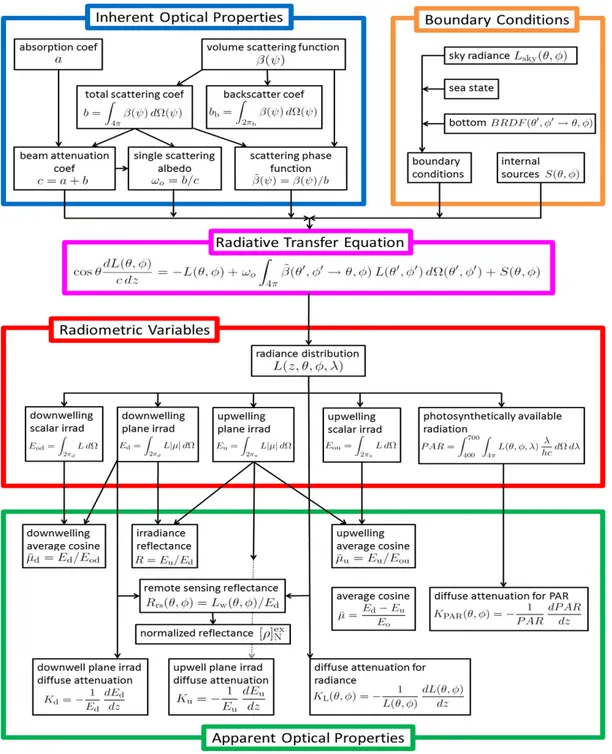
Radiative transfer processes are explicitly dependent on the optical properties of the components in the path between the sun and the ocean and its constituents. Light entering the ocean has only two possible fates; it can be absorbed or scattered. Within this context, it is convenient to classify bulk optical properties of the ocean as either inherent or apparent. Inherent optical properties (IOPs) depend only on the medium and are independent of the ambient light field. The inherent optical properties include the spectral absorption coefficient êÅ(i), spectral scattering coefficientcEÅ(i), and beam attenuation coefficient
DÅ(i) (Smith and Baker, 1978, Kirk, 1994; Mobley, 1994; Spinard et al., 1994). IOPs are additive and for many applications, it is often convenient to partition the total absorption coefficient a, the total scattering coefficient b, and the total beam attenuation coefficient, c, in terms of contributing constituents, namely water, phytoplankton, colored dissolved organic matter (CDOM) and detritus.
Apparent optical properties (AOPs) depend on both the IOPs and the angular distribution of solar radiation (i.e., the geometry of the subsurface ambient light field). Commonly used AOPs are reflectance and various attenuation functions (K functions). To a reasonable approximation, the attenuation of downwelling incident solar irradiance, Q#(i, P), can be described as an exponential function of depth:
Q#(i, P) = Q#(i, 0l)<ëíc[−!
#(i, P)P], (5)
where z is the vertical coordinate (positive downward), Q#(i, 0l) is the value of Q # just
below the air-sea interface, and !#(i, P) is the spectral diffuse attenuation coefficient of
downwelling irradiance. !#(i) (depth dependence is suppressed) is one of the important AOPs. The contributions of various constituents (e.g., water, phytoplankton, detritus and CDOM) to !#(i) are often represented in analogy to their absorption coefficients. This leads to the term quasi-inherent optical property. However, a key point is that !#(i) is
dependent on the ambient light field. It should be noted that for low sun angle and/or when highly reflective organisms or their products (e.g., coccolithophores and coccoliths) are present, multiple scattering becomes increasingly important and simple relations between IOPs and AOPs break down. The relationships between IOPs and AOPs are central to developing quantitative models of spectral irradiance in the ocean. Radiative transfer theory provides the mathematical formalism for linking IOPs and the conditions of the water environment and light forcing to the radiometry and AOPs of the water column (Gordon, 1994; Kirk, 1994; Mobley, 1994; Spinard et al., 1994).
The bio-optical properties due to their anomalous nature, under low sun elevations (for example in polar regions and during winter, dawn & dusk at a given location) and clouds are different for different latitudinal regions. Hence, a careful assessment of Q# and !# under changing climatic conditions that results in more frequent cloudy days, and under larger solar zenith angles are required based on radiative transfer modeling and in situ measurements.
Figure 4. Schematic representation of the optical properties of the water (cf. Mobley 1995, Ocean Optics Web Book • All contents 2019 Creative Commons Attribution license. Permission is granted to copy, distribute and/or modify this document under the terms of the GNU Free Documentation License, Version 1.2 or any later version published by the Free Software Foundation; with no Invariant Sections, no Front-Cover Texts, and no Back-Cover Texts. A copy of the license is included in the section entitled GNU Free Documentation License).
Impact of light propagation on primary productivity
Marine net primary production (NPP: mg C m-2) is an important measure of health of the
ecosystem and carbon cycling and in general estimated as the product of phototrophic biomass, incident solar radiation, and a scaling parameter to give account of the variations in plant physiology (Behrenfeld et al., 2001). The photosynthetic fixation of inorganic carbon to organic matter is the dominant source of energy for the biosphere. Most marine phototrophs are microscopic and are distributed vertically within a euphotic zone, which extends from the surface to depths and varies depending on light attenuation. Characterization of propagation of the visible light in the upper ocean is significant for the description of many oceanographic processes (Dickey and Falkowski, 2002; Dickey et al., 2011). For example, as one of the most important contributors to the production by phytoplankton on Earth, phytoplankton are very sensitive to the variability of the light field in the upper ocean (Walsh and Legendre, 1983; Falkowski, 1984; Litchman and Klausmeier, 2001). Knowledge of the underwater light field has been largely developed in the context of biological studies (Jitts et al., 1976; Bidigare et al., 1987; Hoepffner et al., 1994; Honda et al., 2009; Smyth et al., 2005) and irradiance is the most characterized descriptor of the light field (e.g. Siegel and Dickey, 1987; Siegel et al., 1995). Several studies were carried on development and validation of primary productivity models utilizing both Satellite Ocean color measurements as well as from the parameterization of irradiance based on radiative transfer modeling and IOPs (Saba et al., 2011, Lee et al., 2015 and references there in) in different regions of world oceans. The biomass for marine plant populations can double in days (Sheldon et al., 1972; Goldman and McCarthy, 1978). The high turnover of marine plants suggests that the day-to-day variability of solar irradiance has the potential to influence more strongly the distributions and production of biomass in the ocean.
Modeling ocean primary production: Relationship between photosynthesis, light
Photosynthesis, being a light-driven process, is described better using accurate light attenuation models. Various factors (chemical, physical, biological) govern the photosynthesis in natural phytoplankton assemblages and phytoplankton production
(Morris et al., 1974; Jones, 1977; Harris et al., 1980). One approach establishes statistical relations between the instantaneous rate of photosynthesis, ïñ(Ö) and the simultaneous
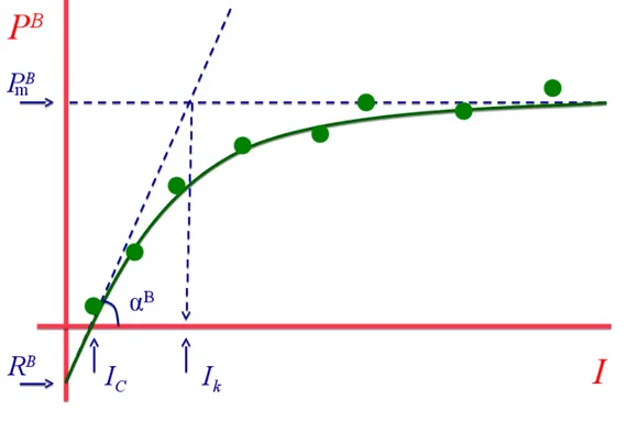
observations of environmental and biological factors that affect it (Platt and Subba Rao, 1970; Platt et al., 1973). This approach in general emphasized the major influence of ambient irradiances on the photosynthetic rate (Fogg, 1975; Platt et al., 1975). An alternate approach, to assess the importance of environmental factors in regulating the photosynthetic rate of natural phytoplankton assemblages is given by parameters describing the light-saturation curve. Photosynthetic-light (P-I) curves are extensively used in primary productivity studies to predict the temporal and spatial variability in the instantaneous rate of photosynthesis due to fluctuations in light intensities (Fig. 5).
Figure 5. Photosynthesis-irradiance curve
An empirical relation between photosynthesis and light, for light intensities lower than the threshold of photo-inhibition, is given by hyperbolic tangent equation (Jassby and Platt, 1976; Platt and Jassby, 1976):
ïñ = c ï
Where bñ is the initial slope of the curve (mg C mg Chla-1 h-1 W-1 m2);
ïzñ is the specific productivity at saturating light (mg C mg Chla-1 h-1);
ôñ is the intercept at zero irradiance.
The above parameters represent the physiological characteristics of phytoplankton and are affected by the changing environmental conditions including light intensity, thus not being constant in space or time (Harris, 1978). But this empirical relation is restricted to the range of light intensities below the threshold of photoinhibition. A modified empirical relation to describe the photosynthesis by phytoplankton as a continuous function of available light from the initial linear response to the highest light levels as influenced under all environmental conditions is given by Platt et al., 1980:
ïñ = c ï
zñ[1 − <ëí àlöõú
ùûé] <ëí à
lüõ
úùûé (7)
The units of all the parameters are same as given above, 5 has the same units as b and it characterizes the photoinhibition. Thus, eqn.7 represents the light-saturation curve throughout the entire range of light intensities in general available to natural phytoplankton assemblages by a single, continuous function of light with the parameters: b, characterizing the photosynthetic photochemical reactions; ïzñ, characterizing the output of the
photosynthesis dark reactions and 5, characterizing the photoinhibition process.
Observation of oceanic light properties from space
Today, satellite-based techniques provide the estimates of surface PAR (Frouin and Marukami, 2007). Without direct contact with the ocean, satellite borne sensors receive and record electromagnetic radiation emanated from the ocean and atmosphere scattered into the space. After removing the effect of the atmosphere, the electromagnetic signal contains information of surface or near-surface oceanic properties and can be interpreted to extract useful information on these properties. The visible part of the electromagnetic spectrum, which spans the wavelengths 400-700 nm (Fig. 1) convey the information of oceanic surface properties. Thus, remote sensing providing the optical view of the ocean is
generally known as ocean color remote sensing. It can collect more complex information than the human eye (Morel, 1980; Robinson, 2004).
Most of the ocean colour sensor satellites are mounted on a near-polar orbits that have orientation of their overhead trajectory around the Earth close to the orientation of the Earth’s polar axis (Robinson, 2004). The sensors view a wide swath of the Earth’s surface by rapidly scanning the surface strip that lies perpendicular to the direction of flight (Kirk, 1994). This capability, together with 700-800 km satellite altitude, commonly used in ocean color remote sensing, yields a swath width ranging from a few hundreds to thousands of kilometers (IOCCG, 1998). During the flight of polar-orbiting satellite above the Earth, the Earth rotates eastward. Therefore, within the satellite repeat cycle, each consecutive orbit covers a different swath. The space borne sensors measure the light signal in a portion of sunlight that reaches the ocean and, rather than being absorbed, gets scattered upward in the sensor direction. Thus, the sensor can view the ocean during sun-lit hours. It takes ~100 minutes to complete an orbit and the observed swath is very wide and the entire ocean surface area can be spanned in one to three days (IOCCG, 1998). However, the presence of clouds conceals the view of ocean surface from satellite ocean color sensors, that extends the global coverage time to about 5-10 days (Campbell et al., 2002). Even with those limitations, ocean colour remote sensing provides better spatial coverage in comparison to field measurements.
The principle of ocean color remote sensing arises from the fact that the behavior of light changes as it passes through the water column due to interaction with sea water and its constituents. Phytoplankton cells, CDOM and suspended matter, are the optically active components of seawater, which obstruct or alter the propagation of photons by absorption or scattering processes (Kirk, 1994) and they interact with light in a characteristic way. Thus, they impose changes on light resulting in the change in the magnitude and spectral composition of the upwelling photon flux, which can be translated into qualitative and quantitative information on the optically active components.
Satellite ocean color sensors measure the magnitude of radiation in multiple distinct narrow bands across the visible domain, this enables the detection of contributions of seawater constituents to the water-leaving light (such as chlorophyll a, PAR, diffuse
attenuation coefficient at 490 nm, Kd(490) etc.,). Ocean color algorithms (empirical,
semi-analytical) that are developed based on theoretical understanding of ocean optics and advances in remote sensing technology can simultaneously derive more than one property (O’Reilly et al., 2000; Boss and Roesler, 2006; Garver and Siegel, 1997; Lee et al., 2002; Loisel and Stramski, 2000; Maritorena et al., 2002; Sathyendranath and Platt, 1997; Smyth et al., 2006; Frouin and Marukami, 2007). However, in the Arctic the frequent occurrence of clouds, especially during late summer and early fall, strongly limits the amount of available ocean color data (Perrette et al., 2011). Thus, the problem of heavy cloudiness in the Arctic, considerably limits the retrieval of biogochemical variables. Sea ice cover limits the spatial coverage and complicates remote sensing of the key variables for PP estimation and also satellite optical sensors do not provide information below the ice (Bélanger et al., 2007) where a large part of (may be 30%, Popova et al., 2010) the annual PP occurs.
Aims and Objectives
In Ocean, shortwave radiation is one of the major physical factors that control the phytoplankton distribution. As mentioned above, surface type, solar elevations, aerosols and clouds impact the solar radiation reaching the surface. Thus, knowledge on light distribution in terms of spectral dowelling irradiance , diffuse attenuation coefficient , and the nature of photosynthesis under varying light conditions using radiative transfer modeling and in situ measurements are needed for the improvement of remote sensing algorithms and primary production models and to quantify the changes in the ecosystem to climate fluctuations and anthropogenic activities.
The central objective of the thesis is to study the variability of quantity and quality of light field under large solar zenith angles, clouds and under highly fluctuating light conditions. Different approaches were evaluated using a combination of in situ datasets, satellite data and the radiative transfer modeling. This will allow us to address the following questions: Chapter 1: How do the large solar zenith angles and cloudy conditions affect estimates of downward irradiance?