HAL Id: pastel-00577855
https://pastel.archives-ouvertes.fr/pastel-00577855
Submitted on 17 Mar 2011HAL is a multi-disciplinary open access archive for the deposit and dissemination of sci-entific research documents, whether they are pub-lished or not. The documents may come from
L’archive ouverte pluridisciplinaire HAL, est destinée au dépôt et à la diffusion de documents scientifiques de niveau recherche, publiés ou non, émanant des établissements d’enseignement et de
Finite element modelling of grain-scale heterogeneities
in polycrystalline aggregates
Héba Resk
To cite this version:
Héba Resk. Finite element modelling of grain-scale heterogeneities in polycrystalline aggregates. Materials. École Nationale Supérieure des Mines de Paris, 2010. English. �NNT : 2010ENMP0047�. �pastel-00577855�
!
"
#
$
!
!"#$!$%$&'(#&#)!(")(#&($&$()*"+,+-!(#École Doctorale n
O364 : Sciences Fondamentales et Appliquées
Doctorat ParisTech
T H È S E
pour obtenir le grade de docteur délivré par
l’École nationale supérieure des mines de Paris
Spécialité « Mécanique Numérique »
présentée et soutenue publiquement parHéba RESK
le 03 décembre 2010Finite element modelling of grain-scale heterogeneities in
polycrystalline aggregates
∼ ∼ ∼
Modélisation par Éléments Finis des hétérogénéités à l’échelle
granulaire au sein d’agrégats polycristallins
Directeur de thèse : Thierry COUPEZ Co-encadrement de la thèse : Roland LOGÉ
Jury
L. DELANNAY,Professeur, iMMC, Université catholique de Louvain Président
A. HAZOTTE ,Professeur, LETAM, Université de Metz Rapporteur
O. CASTELNAU ,Directeur de recherche, PIMM, Arts et Métiers ParisTech Rapporteur
T. COUPEZ,Professeur, CEMEF, MINES ParisTech Examinateur
R. LOGÉ, Docteur, CEMEF, MINES ParisTech Examinateur
M. BERNACKI, Docteur, CEMEF, MINES ParisTech Examinateur
MINES ParisTech Nom de l’Unité de recherche
The Road Not Taken
Two roads diverged in a yellow wood, And sorry I could not travel both And be one traveler, long I stood And looked down one as far as I could To where it bent in the undergrowth; Then took the other, as just as fair, And having perhaps the better claim Because it was grassy and wanted wear, Though as for that the passing there Had worn them really about the same, And both that morning equally lay In leaves no step had trodden black. Oh, I marked the first for another day! Yet knowing how way leads on to way I doubted if I should ever come back. I shall be telling this with a sigh Somewhere ages and ages hence: Two roads diverged in a wood, and I, I took the one less traveled by, And that has made all the difference.
Acknowledgments
Understanding the physics of materials at the microscopic level has always fascinated me and I am very grateful to the Universe for completing my thesis work in this particularly challenging and interesting field. This work, would not have been possible though, without the contribution of a lot of people, who helped me, either on the professional or the personal level, or both.
My first acknowledgements go to the CEMEF and its directors, Jean-Loup Chenot and Yvan Chastel, for recruiting me and giving me the opportunity to achieve this work. Secondly, I would like to thank my thesis advisors Thierry Coupez and Roland Logé as well as my close collaborator Marc Bernacki, for helping me, each in their own way. I owe Thierry my sense of autonomy and my obsession for achieving a clear understanding of the problem at hand. I would like to thank him for his stinging, yet useful remarks, and for giving me the opportunity to be part of the CIM group. I would like to thank Roland for his valuable contributions, especially regarding the physics of the problem and for the numerous discussions we had. I really appreciate Marc’s regular involvement and help in the more numerical aspects of this work. I am grateful for their complementary guidance.
I would like to express my thanks to the members of the jury of this thesis, Pr. Alain Hazotte, Dr. Olivier Castelnau and Pr. Laurent Delannay. Special thanks to Laurent for his con-tributions, help and support I would like to thank the EU for their funding and for allowing me to work with other scientists from European and American universities, who participated in the DIGIMAT project, namely the Centre des Matériaux (CDM) of Mines Paristech, Carnegie Mel-lon University (CMU), Eötvös University (ELTE), Princeton University and Imperial College (IC). Special mention to R. Quey for supplying the experimental data used in chapter 6.
I would like to thank Luisa Silva, Hugues Digonnet and Julien Bruchon of the CIM group for answering my numerous questions and for helping me achieve my goals. My appreciation goes also to all my former colleagues of the CIM group, who nourished my work. I would like to express my gratitude to all the CEMEF staff. Special mention to Gilbert Fiorucci, Bernard Triger, all people from the workshop for their lovely spirit, the IT department team (EII), who always solved my problems in a timely manner and the CEMEF’s administrative director Patrick Coels for his availability. The Ladies of the CEMEF played an important role in making my life easier on campus, professionally and personally. Special thanks to Marie-Francoise, Sylvie,
Suzanne, Genevieve, Florence, Carole, Murielle and the librarians Brigitte and Sylvie.
On a more personal note, I would like to express my thanks to all the other Phd students and postdoctoral researchers, my former office colleagues and friends Christelle, Toufik, Mon-ica, Guillaume and Greg. Special mention to the former members of the ATS and Mines Sport Valbonne, which I presided during my stay, the members of the small choir that we have created, and finally the salseros and the salseras of the Riviera.
Last but not least, I would like to thank the people who helped me see the light at the end of the tunnel, namely “number 47”, my high school and university friends. To the dearest people to my heart, my father, my mother, Mimi, Momo, Tati, Gougou and the rest of the family, who provided love and support from nearly 2000 miles away, I dedicate this thesis. I wouldn’t have made it without them.
Abstract
Macroscopic properties of crystalline solids depend inherently on their underlying mi-croscopic structure. Studying the mechanisms operating at the microstructural scale during the various thermomechanical processes to which such materials may be subjected offers a valuable insight into their final in-use properties. The objective of this work is to investigate grain scale heterogeneities in polycrystalline aggregates subjected to large strains using the Crystal Plasticity Finite Element Method (CPFEM). For this purpose, highly resolved simu-lations, where each grain is represented explicitly, are needed. The first part of this work is devoted to a detailed account of the numerical framework implemented for such simulations. A classical elastic-viscoplastic crystal plasticity model is combined to a non-linear parallel finite element framework. The discretization of the digital microstructures is performed using non-conforming unstructured meshes. Most importantly, a level set approach is used to describe grain boundaries and to guide an adaptive anisotropic meshing strategy. Automatic remeshing, with appropriate transport of variables, is introduced in the proposed framework. In the second part of this work, the robustness and flexibility of our approach is demonstrated via different CPFEM applications. The deformation energy is used to assess heterogeneities in polycrys-talline aggregates, highlighting the need to perform adaptive meshing so as to achieve a good compromise between accuracy and computation time. These grain-scale heterogeneities are to be accurately predicted during the deformation simulation if subsequent static recrystallization modelling is to be performed. An example of linking between the deformation and static re-crystallization steps, using the proposed common approach, is illustrated. In terms of global texture predictions, the CPFEM framework is validated for a highly resolved model polycrys-tal subjected to more than 90 % thickness reduction in rolling. The importance of automatic remeshing in avoiding excessive mesh distortion, in such applications, is demonstrated. Most importantly, microtexture analysis is performed on digital microstructures that correspond, in a discrete sense, to an actual microstructure observed experimentally. Intragranular misori-entation predictions and virtual 2D orimisori-entation maps are compared to the experimental ones, highlighting the difficulties pertaining to the validation of such grain-scale predictions.
Résumé
Les matériaux cristallins, notamment métalliques, sont des matériaux hétérogènes. Leurs propriétés macroscopiques sont fondamentalement déterminées par leurs caractéristiques mi-crostructurales. L’étude des mécanismes opérant à l’échelle du grain permet de mieux com-prendre et ainsi mieux contrôler les caractéristiques des pièces fabriquées afin de réduire leur coût et optimiser leur performance.
Cette thèse s’inscrit dans le cadre de la méthode dite “CPFEM” qui couple la plastic-ité cristalline à la méthode des Éléments finis (EF). L’objectif de ce travail est d’étudier les hétérogénéités à l’échelle du grain au sein d’agrégats polycristallins soumis à de grandes dé-formations. Pour ce faire, une représentation explicite de la microstructure est nécessaire. Le travail réalisé, ainsi que ce manuscrit, s’articule autour de deux axes principaux: (i) la mise en place d’un cadre numérique robuste adapté à des calculs intensifs en grandes déformations; (ii) la validation de ce cadre à travers différents cas tests, qui permettent, notamment, d’étudier les hétérogénéités locales.
Dans le chapitre 2, le comportement du matériau est modélisé par une loi élastoviscoplas-tique cristalline, qui ne prend cependant pas en compte le développement d’une sous-structure dans sa formulation. Cette loi est couplée à une formulation EF mixte en vitesse pression. L’approche EF, détaillée dans le chapitre 3, peut être considérée comme le modèle polycristallin idéal vu le respect, au sens numérique faible, de l’équilibre des contraintes et la compatibilité des déformations. Dans le chapitre 4, l’approche utilisée pour construire, représenter et discré-tiser un volume polycristallin est détaillée. La microstructure est représentée, soit par des polyè-dres de Voronoi, soit par des voxels, si elle est construite à partir de données expérimentales. L’agrégat polycristallin est discrétisé avec une approche “monolithique”, où un seul maillage, non structuré et non-conforme aux interfaces entre les grains, est utilisé. Une approche level set permet alors de décrire l’interface entre les grains de façon implicite et sert de base pour la construction d’un maillage adaptatif anisotrope. Le remaillage, avec un transport approprié des variables du problème, se fait de façon naturelle et automatique si la carte de métrique, associée au maillage, est calculée avant la procédure de remaillage.
la déformation. Une analyse de sensibilité, au degré et au type de maillage utilisé, permet de mettre en évidence l’apport d’une stratégie de maillage anisotrope. Ces données locales sont particulièrement importantes à calculer lors de la déformation d’agrégats polycrystallins si l’objectif est de modéliser le phénomène de recristallisation statique qui suit l’étape de défor-mation. Un cas test 3D permet d’illustrer le cha”nage de la simulation de la déformation et de la recristallisation, toutes deux réalisées dans le même cadre numérique.
Dans le chapitre 6, notre approche numérique est, dans un premier temps, validée à l’aide d’un cas test de laminage pour un polycrystal statistiquement représentatif d’une texture expéri-mentale. Une réduction d’épaisseur de plus de 90 % est réalisée. Le remaillage, dans ce type d’application, s’avère plus que nécessaire. Dans la seconde partie de ce chapitre, une étude approfondie de la microtexture, développée au sein de microstructures virtuelles, est effectuée. Dans ce cas, ces microstructures “digitales” correspondent à une microstructure réelle dans un sens discret. Les prédictions de désorientations, d’orientations cristallographiques moyennes ainsi que les cartes d’orientation 2D virtuelles, sont comparés à l’expérience à l’échelle de chaque grain, mettant ainsi en évidence les facteurs à l’origine de certaines des différences observées.
Contents
1 Introduction 12
I Micromechanical modelling of polycrystalline materials . . . 12
II Experimental characterization and investigation at the grain scale: the limits . . 15
III Objectives of the present work and thesis outline . . . 17
2 Single crystal plasticity 20 I Components of a single crystal model . . . 21
II Flow rule . . . 22
II.1 Ideal plastic flow . . . 22
II.2 Viscoplastic flow . . . 24
III Hardening . . . 25
III.1 Proportional hardening . . . 25
III.2 Latent hardening . . . 26
III.3 Including kinematic hardening . . . 26
III.4 Using dislocation densities and including gradient effects . . . 27
IV Single Crystal model used in this work . . . 29
IV.1 formulation . . . 29
IV.2 Time integration scheme of the constitutive law . . . 32
V Conclusion . . . 33
3 Accounting for grain interaction 35 I Polycrystal theories . . . 35
I.1 Sachs model . . . 36
I.2 Taylor full-constraint model (FC) . . . 36
I.3 Relaxed constraints models (RC) . . . 37
I.4 N-site models . . . 38
I.4.1 The LAMEL model . . . 38
III Finite element formulation in this work . . . 43
III.1 Balance laws . . . 43
III.2 Variational formulation . . . 44
III.3 Time discretization . . . 45
III.4 Spatial discretization . . . 45
III.4.1 The MINI-element . . . 46
III.4.2 The discrete problem . . . 47
III.5 Resolution . . . 49
III.5.1 Non linear system of equation to be solved . . . 49
III.5.2 Resolution of the non linear system . . . 49
III.5.3 General solution procedure and numerical implementation . . 51
IV Conclusion . . . 52
4 Generating and Meshing polycrystalline aggregates 53 I Microstructure generation and meshing overview . . . 53
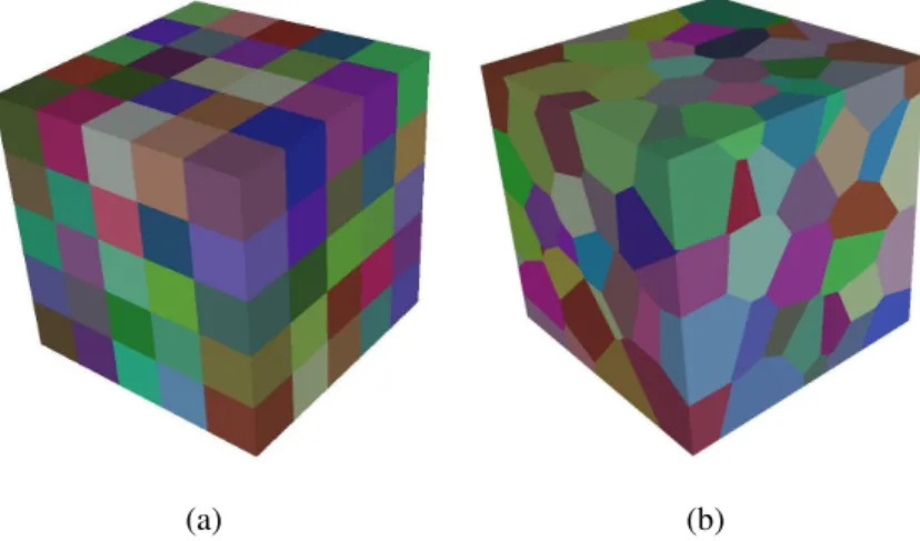
II Generating digital microstructures . . . 56
III From geometrical representation to FE computations . . . 59
III.1 Initial mesh generation . . . 59
III.2 Level-set framework for grain representation . . . 60
III.3 Mesh adaptation . . . 62
III.3.1 Metric definition . . . 62
III.3.2 Anisotropic mesh adaptation . . . 63
III.4 Microstructural variable assignment . . . 65
III.5 Remeshing . . . 66
III.6 Boundary conditions . . . 69
IV Conclusion . . . 70
5 Stress and strain rate heterogeneities: investigation & application 71 I Overview of Recrystallization modelling . . . 72
I.1 The physics: importance of deformation history . . . 72
I.2 Approaches to recrystallization modelling . . . 73
I.3 Linking deformation and recrystallization simulations . . . 74
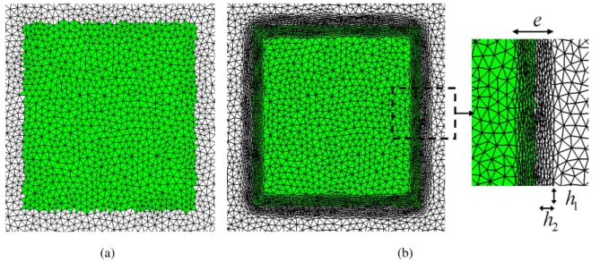
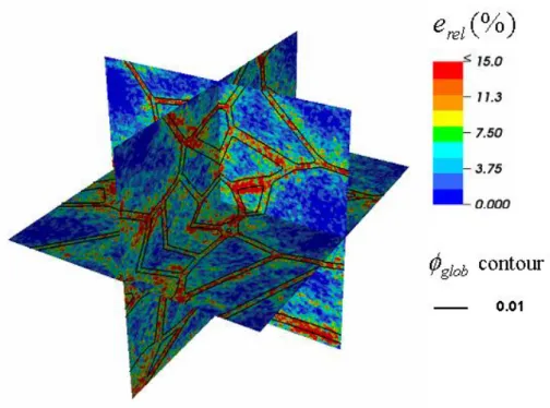
II Effect of mesh type, mesh refinement and remeshing in highly resolved poly-crystalline simulations . . . 76
II.1 Error Analysis . . . 78
II.2 Mesh size effects . . . 79
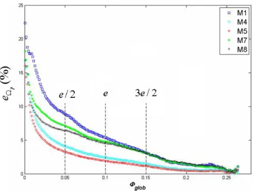
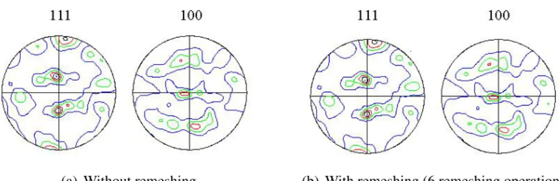
II.3 Remeshing Effects . . . 84
III Deformation and recrystallization simulation test case . . . 86
III.2 Simulation of deformation and subsequent recrystallization . . . 88
IV Conclusion . . . 91
6 Deformation texture prediction 93 I Orientation . . . 93
I.1 Orientation description . . . 93
I.2 Orientation representation . . . 95
I.3 Texture analysis . . . 96
II Misorientation . . . 98
II.1 Basic definition . . . 98
II.2 Some misorientation measures . . . 98
II.2.1 Disorientation . . . 98
II.2.2 Orientation deviation . . . 99
II.2.3 Local misorientation . . . 99
III Orientation image microscopy . . . 101
IV Prediction of macrotexture in a model polycrystal . . . 103
V Detailed comparison between FE simulations and measured microstructure evo-lutions . . . 106
V.1 Experimental Setup . . . 106
V.2 Simulations setup . . . 107
V.3 Effect of the surrounding medium . . . 109
V.3.1 Global texture evolution . . . 113
V.3.2 Grain subdivision predictions . . . 120
V.3.3 Average orientation predictions and orientation deviation dis-tributions for the first ten grains . . . 123
V.4 Effect of mesh refinement and microstructure type . . . 128
V.4.1 Global texture evolution . . . 129
V.4.2 Grain subdivision predictions . . . 133
V.4.3 Average orientation predictions and orientation deviation dis-tributions for the first ten grains . . . 135
V.4.4 Link between fragmentation and mean orientation predictions for the first ten grains . . . 138
VI Conclusion . . . 151
7 General conclusion and perspectives 154
C Stress and strain heterogeneities for different HEM approximations (chapter 6) 230
Chapter 1
Introduction
I Micromechanical modelling of polycrystalline materials
Metallic materials exhibit a crystalline structure and are in essence heterogeneous mate-rials. They are in fact polycrystals, composed of several crystals or grains. These latter are defined as regions of continuous lattice orientation. At a lower scale, as seen on figure 1.1, one finds dislocations, which are linear defects in the crystal lattice, which is otherwise a perfect arrangement of atoms.
Fig. 1.1: From sample level to atoms
Crystal plasticity theory [Kocks, 1998a] provides a first level of linking between macro-scopic properties and micromacro-scopic features (crystallographic orientation...). It is intended to represent the behavior of polycrystals at the mesoscopic scale without modelling explicitly the motion of individual dislocations or individual atoms, which are the concern of dislocation dynamics models and atomistic models. During processing, metallic parts are subjected to var-ious thermomechanical treatments. Microstructural evolution triggered by plastic deformation
• from a technological point of view, assist the design of thermomechanical processes by taking into consideration these microstructural features, such as crystallographic orien-tation, in order to account for macroscopic anisotropic behavior such as the earing in deep-drawn aluminum cans (fig. 1.2),
• from a more fundamental point of view, increase our understanding of the mechanisms operating at the microstructural scale.
Fig. 1.2: Earing in aluminum cans [AluMATTER, 2009]
Although first simulations based on crystal plasticity were initiated a while ago, with the pioneering work of Pierce and co-workers [Peirce et al., 1982, 1983], their added-value for the understanding of macroscopic anisotropy has not been fully apprehended as their development is directly linked to improvements in computational methods and optimization of computational resources. In real-scale Finite Element (FE) simulations of metal forming processes like in figure 1.3(a), each material point (integration point) represents a set of crystals i.e orientations with no account for topological arrangement of grains or for their shapes. In such formulations, a polycrystal model is needed in order to link the micro and the macro scales. The chosen transition rule could be more or less satisfactory in terms of deformation compatibility and stress equilibrium, depending on the way the interaction between the grains is accounted for. These two-level models are then used in much the same way as any other macroscopic constitutive law, but providing better predictions of the final mechanical properties of the sample [Dawson et al., 1994; Delannay et al., 2005; Kalidindi et al., 1992].
Crystal plasticity theory can also be used in“small scale” FE simulations, in which the grains are represented explicitly (fig. 1.3(b)). In this case, the microstructure could either represent a model polycrystal in a statistical sense, or, in some specific cases, an actual mi-crostructure observed experimentally. Small scale FE simulations can be assimilated to in-situ observations performed during virtual mechanical testing. They can be very useful for studying the local micro-mechanical fields that develop within a polycrystalline aggregate subjected to loading. It should be noted that a relatively recent approach based on the Fast Fourier Trans-form (FFT) algorithm has been adapted to compute the deTrans-formation of viscoplastic 2D and 3D polycrystals [Lebensohn et al., 2008, 2005]. This approach seems to be a viable alternative to the FEM but is however limited to viscoplastic behaviors. Other limitations associated with
this approach are the boundary conditions, which are are necessarily periodic, and the mesh ( structured grid) which does not deform. The FEM remains the most widely used procedure in the domain of small scale crystal plasticity simulations due to its versatility and robustness. Compared to polycrystal models, the FE approach does not obviously require a transition rule, as the scale at which the simulation is performed is actually the grain’s scale. The Crystal Plas-ticity Finite Element Method, also known as CPFEM, has been used extensively in the last two decades[Bate, 1999]. Numerous examples are found in the literature [Barbe et al., 2001a,b; Mika and Dawson, 1998; Sarma et al., 2002] and could be differentiated on the basis of, on the one hand, their intended objectives and, on the other hand, the crystal plasticity models, the FE formulation and the numerical tools used to represent and mesh the microstructure. Due to its inherent nature, FE results are obviously quite sensitive to microstructure representation and mesh discretization. Depending on the intended objectives and the computational limitations, the use of different numerical strategies is justified. In effect, one can be interested in sev-eral types of analyses, which can be classified in two main categories:(i) predicting the global response of the polycrystal such as the stress-strain curve or the ODF or other global texture evolution measurements; (ii) focusing on the local heterogeneities of stress, strain and lattice orientation . It should be noted that care should be taken while interpreting the huge amount of microstructural data that can be extracted from such simulations. The presence of a large variety of approaches could hinder the formulation of general conclusions. This is all the more true because of the difficulties pertaining to the validation of such micromechanical predictions against experimental measurements.
(a) (b)
Fig. 1.3: Real-scale and small scale FE simulations: (a) simulation of deep drawing process using polycrystal plasticity [Rousselier et al., 2009]; (b) A meshed polycrystal made of 17 grains [Maniatty et al., 2007]
II Experimental characterization and investigation at the grain
scale: the limits
The validation of the results of small scale simulations entails first the ability to generate virtual 3D microstructures that correspond to the real microstructures and then to compare the numerical predictions to relevant experimental results. The construction of the microstructure is in fact a challenge, whether the digital microstructure is intended to represent a model polycrys-tal or an actual microstructure observed experimenpolycrys-tally. Two distinct but complementary types of information are needed to fully describe a polycrystal: geometric features regarding grain morphology and topology and the corresponding spatial distribution of physical quantities like the crystallographic orientation. In the case of a model polycrystal, the digital microstruc-ture is considered representative of the real material if it contains a sufficient number of grains and if it matches the real material in a statistical sense both in its geometrical ( morphology-topology) features and in the spatial sampling of its physical attributes. In the case of an exact microstructure replicate, these microstructural features have to be respected in a discrete and exact sense. While the numerical algorithms needed to fit experimental data are far from be-ing perfect [Bhandari et al., 2007; Rollett et al., 2007], the first limitbe-ing factor regardbe-ing the construction of digital polycrystals lies in the actual 3D characterization of the microstructure before deformation and whether or not such characterization is destructive. There are essentially two methods available nowadays for characterizing microstructures in 3D: 2D sectioning based on electron back-scatter diffraction (EBSD), also known as orientation imaging microscopy (OIM), and 3D X-ray diffraction (3DXRD) microscopy.
Fig. 1.4: Example of a model polycrystal: voxelization of a rolled microstructure including crystallographic orientation data based on the Microstructure Builder approach (Carnegie Mel-lon University) [Brahme et al., 2006]
In orientation imaging microscopy, thin successive layers of the material are polished and scanned using EBSD and the obtained regular pixelized grids are then assembled to obtain the
final 3D microstructure [Erieau, 2003; Gosh et al., 2008]. Without dwelling on the difficulties pertaining to the alignement of the successive layers, the major drawback of such technique is related to its destructive nature. In the same vein, the Microstructure Builder approach [Brahme et al., 2006] is based on EBSD scans of two orthogonal planes (fig. 1.4). While this approach optimizes the scanning effort, it is only pertinent if the digital microstructure is to represent a model polycrystal. Indeed, if this is the objective, then the destructive nature of these two meth-ods are insignificant as the simulation predictions can be compared to any other specimen of the same polycrystal. On the other hand, in the case of "real" microstructures, researchers have also used EBSD scans in order to follow the same set of grains before and after deformation. Due to the 2D nature of the scans, these studies were sometimes limited to multicrystalline specimens, where the microstructure is essentially composed of one layer of crystals [Delaire et al., 2000; Kalidindi et al., 2004]. In other cases, authors have confined their investigations to the layer located on the free surface of the specimens [Buchheit et al., 2005; Lebensohn et al., 2008] while "guessing" the rest of the microstructure. The split sample method, originally introduced in the early 40’s [Barrett and Levenson, 1940] and more recently adapted and perfected to channel die compression [Panchanadeeswaran et al., 1996; Quey, 2009], is used to follow the grains in the bulk of the polycrystalline specimens. Nevertheless, the indetermination regard-ing the surroundregard-ing microstructure remains a problem if 3D simulations are compared to such measurements.
3D X-ray diffraction microscopy (fig. 1.5) is a non destructive technique currently used to follow grains in the bulk of millimeter-centimeter thick polycrystals [Sørensen et al., 2006]. This tool can be considered as state-of-the-art technique in the characterization of grains and sub-grains. It has been used to follow grain growth in annealed specimens [Sørensen et al., 2006] and the deformation of grains inside specimens subjected to relatively low strains [Poulsen et al., 2003]. The low strain limitation is due to the fact that all the grains diffract at the same time and excessive grain fragmentation leads to overlapping of diffraction spots.
III Objectives of the present work and thesis outline
In this work, a CPFEM modelling strategy is used to approach the micromechanics of polycrystalline aggregates. In Chapter 2, modeling assumptions about single crystal behavior are reviewed briefly before presenting the actual single crystal model used in this study, thus highlighting the limits of the chosen approach. The model used is a classical elastic-viscoplastic formulation that satisfies the basic objective of taking into account crystal plasticity theory while minimizing the important computational cost that could be associated with a more complex model.
Given the behavior of the single crystal, the different ways to account for the behavior of the polycrystal are reviewed in Chapter 3, namely classical polycrystal plasticity theory and more advanced models that strive to fill the gap between the actual physics behind grain deformation and the simplified modelling assumptions of classical models. In that scope, the FE approach is presented as a limiting case as no assumption is made about grain interaction. Different FE formulations found throughout the literature are briefly reviewed before presenting the framework used in this work, whereby 3D polycrystals are deformed using an updated Lagrangian scheme. This framework is implemented in a parallel multi-component C++ library, called CimLib, developed in CEMEF [Digonnet et al., 2007].
Generating and meshing the microstructure is a pre-requisite for performing FE simu-lations. In Chapter 4, different meshing strategies are highlighted. In this work, a specific approach is introduced, namely an unstructured “monolithic” mesh is used, not necessarily conforming to actual grain boundaries, while a level set framework is used to implicitly lo-cate grains. Adaptive meshing techniques, based on this level set description, is used to define precisely the interfaces of the grains while optimizing computation time. Most importantly, au-tomatic remeshing is introduced as a necessary tool for reaching important strains (true strain > 1). Such strains are typically encountered in metal forming processes like rolling for example.
In Chapter 5, applications of the proposed framework for the investigation of local stress and strain heterogeneities is illustrated. The deformation energy measure is used as a parameter to assess such heterogeneities. Energy that is stored in the material during deformation is the driving force for further microstructural evolution that takes place during deformation or an-nealing. Dynamic or static recrystallization phenomena inevitably occur. Complex multi-scale models are in theory necessary for accurately describing the deformation and the associated recrystallization phenomena [Log´e et al., 2008]. However, before moving to such complicated schemes, one of the first bottleneck to overcome is the ability to transpose all the deforma-tion simuladeforma-tion results to the recrystallizadeforma-tion simuladeforma-tion. In Chapter 5, such linking between deformation simulation and recrystallization simulation is illustrated. The common numerical framework used for both is shown to be an elegant way of achieving this.
Chap-ter 6, a brief overview of crystallographic texture measures and representations is given. Global texture prediction (“macrotexture”) is investigated in a model polycrystal deformed by plain strain compression up to 90 % thickness reduction. Such strain levels can only be obtained if proper remeshing operations are performed at regular intervals. The rest of the chapter is dedi-cated to the investigation of lattice orientation heterogeneities in an experimental microstructure deformed by channel die compression. The experimental part of this investigation has been per-formed by R. Quey from the Ecole Nationale Supérieure des Mines de Saint Etienne [Quey, 2009] who followed the microtexture evolution of individual grains in the bulk of a polycrys-talline aluminum sample. One of the objectives of this chapter is to evaluate the ability of our CPFEM framework to allow the construction of the “equivalent” virtual test and to assess its microtexture predicting capability. Different assumptions are made on the constitutive behavior of the surrounding material due to the lack of experimental data. Highly resolved 3D simu-lations are performed and the OIM software is used to probe a slice of the virtual specimen. Virtual OIM maps are compared to experimental ones and a discussion is held on the topo-logical distribution of orientation gradients and the possibility to predict them with a standard crystal plasticity based constitutive law.
This work is part of the DIGIMAT project (EU/NSF) which aims at developing a frame-work for a thorough understanding and simulation of static recrystallization. Other academic partners include Centre des Matériaux (CDM) of Mines Paristech, Carnegie Mellon University (CMU), Eötvös University (ELTE), Princeton University and Imperial College (IC). The work in this thesis has contributed to the following written communications:
• Log´e, R., Resk, H., Sun, Z., Delannay, L., and Bernacki, M. (2010). Modelling plastic deformation and recrystallization of polycrystals using digital micro-structures and adap-tive meshing techniques. In Proceedings Metal Forming 2010, submitted for publication in Steel Research international
• Resk, H., Delannay, L., Bernacki, M., Coupez, T., and Log´e, R. (2009). Adaptive mesh refinement and automatic remeshing in crystal plasticity finite element simulations. Mod-elling and Simulation in Materials Science and Engineering, 17(7):075012
• Bernacki, M., Resk, H., Coupez, T., and Log´e, R. (2009). Finite element model of primary recrystallization in polycrystalline aggregates using a level set framework. Modelling and Simulation in Materials Science and Engineering, 17(6):064006
• Bernacki, M., Chastel, Y., Digonnet, H., Resk, H., Coupez, T., and Log´e, R. (2007a). Development of numerical tools for the multiscale modelling of recrystallization in metals based on a digital material framework. Computer Methods in Material Science, 7:142– 149
• Bernacki, M., Digonnet, H., Resk, H., Coupez, T., and Log´e, R. (2007b). Development of numerical tools for the multiscale modelling of recrystallization in metals, based on a digital material framework. In Materials Processing and Design: Modeling, Simulation and Applications, AIP conference proceedings, NUMIFORM 2007, volume 908, pages 375–380, Porto, Portugal
and the following oral communications:
• Resk, H., Bernacki, M., Chastel, Y., Coupez, T., Delannay, L., and R.Log´e (2008a). Numerical modelling of plastic deformation and subsequent primary recrystallization in a polycrystalline volume element, based on a level set framework. In WCCM8-ECCOMAS 2008, Venice, Italy
• Resk, H., Bernacki, M., Coupez, T., Delannay, L., and R.Log´e (2008b). Adaptive mesh refinement in crystal plasticity finite element simulations of large deformations in poly-crystalline aggregates. In ICOTOM 15, Pittsburgh PA, USA
Chapter 2
Single crystal plasticity
In crystal plasticity theory, plastic deformation is modelled using the slip system activity concept. Dislocations are assumed to move across the crystal lattice along specific crystallo-graphic planes and directions. As the material is subjected to loading, the applied stress resolved along the slip direction on the slip plane initiates and controls the extent of dislocation glide. This latter has the effect of shearing the material, while the volume remains constant and the crystal lattice remains unchanged. Moreover, the crystal lattice can deform elastically, but elas-tic strains are small compared to plaselas-tic strains and are sometimes neglected in crystal plaselas-ticity models. Finally, the crystal lattice can also rotate to accommodate the applied loading. This lattice rotation (or spin), is responsible for texture development. The concept of lattice rotation in crystal plasticity is not, at first hand, easy to grasp, especially compared to material rotation (or rigid body rotation). [Peeters et al., 2001] illustrate well this fundamental difference with figure 2.1.
Fig. 2.1: “(a) and (b) A shear γ on a slip plane does not cause the lattice to rotate, although a material vector may rotate; (b) and (c) An additional rotation - which also causes the crystal
These considerations form the basics of classical crystal plasticity theory. Other modes of deformation in polycrystals like twinning or grain boundary sliding are not tackled in this discussion. Also, more recent concepts in crystal plasticity modelling, attempting to account for the discrete nature of dislocation glide (non-local theory) are briefly highlighted in section III.4.
I Components of a single crystal model
In order to account for the mechanics of grain structure heterogeneous deformation, crys-tal plasticity models are based on microstructural variables such as cryscrys-tallographic orientation or dislocation densities. Polycrystal models are based on single crystal models as illustrated by figure 2.2 and are discussed in the next chapter.
Fig. 2.2: From Polycrystal level to slip system level
In order to describe the behavior of a single crystal, three components are needed:
1. A kinematic framework describing the motion of the single crystal. The kinematic composition used in crystal plasticity is in the majority of models a multiplicative de-composition as opposed to an additive dede-composition which is generally used for small deformations [Shabana, 2008]. In classical plasticity theory, if the elastic behavior is considered, the decomposition is composed of a plastic and an elastic term.
2. Elastic relations describing the elastic behavior depending on the crystal structure of the material. Elastic strains are small compared to plastic ones but are sometimes important to consider if the objective of the simulations is to compute residual stresses for example [Marin and Dawson, 1998a]. The assumption of small elastic strains enables nevertheless
simplifications in the governing equations [Marin and Dawson, 1998b]. In other applica-tions where elasticity is not a concern, the elastic behavior is neglected [Beaudoin et al., 1995].
3. Evolution rules for the intragranular variables of the model, namely a flow rule and a hardening rule. Different forms of these equations can be found in the literature and a brief overview is given in this section.
II Flow rule
The Schmid law [Schmid and Boas, 1935] determines the resolved stress on slip system α ,i.e the shear stress τα as follows:
τα = T : Mα =T : (bα⊗ nα)S ym , (2.1)
where T is the applied stress, bα is the slip direction, nα is the slip plane normal, Mα is the
Schmid tensor which is the symmetric part of the orientation tensor tα = (bα⊗ nα).
II.1 Ideal plastic flow
At low homologous temperatures, the behavior of single crystals is assumed to be ideally plastic. In this case, the flow is modelled using the Schmid yield criterion. The Schmid yield criterion or the “generalized Schmid law” postulates that yield occurs on a given slip system α if the resolved stress on this slip system (τα) reaches a critical value (τα
c) [Kocks, 1998a]. It can
be expressed as follows: τα = τα c ˙ τα >0 ⇒ ˙γα >0 . (2.2)
where ˙γα is the slip rate for slip system α. This yield criterion defines a yield surface which
indicates the direction in which the flow occurs, i.e the straining direction, for a given stress state. The yield surface is in fact a five dimensional convex polyhedron in stress space, with each facet corresponding to the activation of a single slip system. Straining occurs along the normal to the facets of this polyhedron. At the vertices, the straining direction is undetermined and is bounded by the normals to the facets intersecting at those vertices. Figure 2.3 illustrates the concept in a 2D projection of the stress space.
(a) (b) (c)
Fig. 2.3: 2D projection of yield surface in stress space (a) single slip representation; (b) multiple slip representation;(c) rate independent vs rate dependent plasticity [Kocks, 1998a]. Here s stands for slip system and m is the Schmid tensor
The vertices correspond to a case where more than one slip system is activated, i.e a case of multiple slip. In Taylor’s analysis [Taylor, 1938], five independent slip systems are in fact required to accommodate a given deformation rate (taking into consideration the incompress-ibility condition). Taylor also proposed a way of solving the indetermination regarding the straining direction, i.e regarding the selection of the active slip systems that operate for a given vertex stress state. Assuming that all slip systems have the same initial critical resolved shear stress and that they all harden equally, he postulated that the active slip systems are the ones which minimize the energy dissipated during slip (minimum internal work principle). This can be formulated as follows: � α τα|˙γα| ≤� α τα|˙γα∗| , (2.3) � α |˙γα| ≤� α |˙γα∗| , (2.4)
where ˙γα∗is any possible set of slips satisfying the incompressibility condition.
Later on, in order to solve the same indetermination, Bishop and Hill looked at the prob-lem from the stress point of view, i.e one is to find the stress state that allows for multiple slip. In their analysis, the “correct” stress σ is the one that maximizes plastic work (maximum work principle). This can be formulated as follows:
(σ − σ∗) : E ≥ 0 , (2.5)
where E is the applied strain tensor and σ∗is any possible stress state that activates a minimum
of five slip systems. It has been shown that Taylor’s minimimum internal work principle is actually equivalent to the maximization principle of the plastic work but only if hardening is taken equal for all slip systems [Bishop and Hill, 1951]. For this reason, Taylor’s analysis and Bishop and Hill’s analysis are described as the “Taylor-Bishop-Hill model”.
Ideal plasticity, also known as multi-surface plasticity or “rate independent plasticity”, has been used since in numerical applications [Anand and Kothari, 1996; Knockaert et al., 2000; Peirce et al., 1982; Schmidt-Baldassari, 2003]. Robust numerical procedures are needed for selecting the active slip systems and avoiding singular matrices related to the non-uniqueness of the set of active slip systems. Additional constitutive assumptions are also needed to compute the actual amount of slip on the selected systems. It is important to mention that the robustness of the numerical schemes used in rate independent formulations depends on the chosen hard-ening law, which completes the constitutive framework [Busso and Cailletaud, 2005], and is discussed in section III.
II.2 Viscoplastic flow
Two reasons motivate the use of a viscoplastic form for the flow rule: (i) describing the behavior of metals exhibiting rate sensitivity, especially in applications where localization phenomena is studied, (ii) avoiding the previously mentioned difficulties associated with rate independence . As seen on figure 2.3(c), the use of a rate dependent formulation has the effect of rounding the yield surface, thus avoiding the vertex indetermination. Typically, the viscoplastic behavior is described by an exponential law, first introduced by [Hutchinson, 1977]:
˙γα = ˙γ0 �� �� ��τ α τα c �� �� �� 1/m sign(τα) , (2.6)
where τα is the resolved shear stress, ˙γ
0is a reference slip rate, m the rate sensitivity exponent,
and τα
c the critical resolved shear stress for slip system α. Clearly, this expression assumes that
all slip systems are active and the slip rates (slip increments) are directly determined. Rate independence corresponds to the limiting case when m → 0 and can therefore be theoretically approximated using this expression. Nevertheless it is worth mentioning that, when m is very small, the convergence of the numerical integration scheme of the constitutive equations is more difficult as highlighted by [Anand and Kothari, 1996]. The computational costs of a rate dependent formulation compared to the rate independent one could therefore be more important [Delannay et al., 2002] depending on the adopted value of m.
Equation 2.6 has been frequently used since [Delannay et al., 2006; Erieau and Rey, 2004; Marin and Dawson, 1998b]. This type of flow rule can also be expressed in terms of variables such as dislocation densities thus relating it to more elementary physical mechanisms of the theory of crystal plasticity [Fivel, 1997]. In the same vein, [Cheong and Busso, 2004; Cheong et al., 2005] base their flow rule on the thermally activated motion of dislocations:
˙γα = ˙γ 0 � −κTF0 � 1 − � |τα| − Sαµ/µ 0 ˆτ0µ/µ0 �p�q� sign(τα) , (2.7)
From a more phenomenological perspective, the flow rule introduced by [Cailletaud, 1987] and used later on by several authors [Barbe et al., 2001a; Diard et al., 2005], is given by:
˙γα = � |τα− xα| − rα K �1/m sign(τα− xα) , (2.8)
where K is a material parameter, rα is an isotropic hardening variable and xα is a kinematic
hardening variable.
III Hardening
In order to complete the constitutive framework, hardening has to be taken into account. The hardening rule represents the strain-induced evolution of the material resistance to plastic deformation. It can take the following generic expression:
˙τα c =
� β
hαβ���˙γβ��� , (2.9)
where the hαβ terms are the components of the hardening (modulus) matrix. The hardening
(modulus) matrix reflects the dependence of hardening upon the history of slip, more
specifi-cally on the shearing rate on the different slip systems. The diagonal terms hααaccount for the
hardening of slip system α due to its own slip activity, i.e. self-hardening. The off-diagonal elements hαβ|
α�β reflect the hardening of slip system α due to the slip activity on the slip
sys-tem β, i.e latent hardening. The hardening matrix can have different forms depending on the actual physical mechanisms and phenomenological behaviors that are accounted for and the simplifying assumptions adopted. Proportional and latent hardening are presented below. More elaborate expressions including kinematic hardening and gradient effects are then briefly dis-cussed.
III.1 Proportional hardening
An example of proportional hardening is Taylor’s model. In this latter, all components of the hardening matrix are taken equal and are constant over time:
hαβ = h . (2.10)
The hardening is said to be isotropic as all system harden at the same rate (isotropic hardening). More specifically, in Taylor’s original work, the critical resolved shear stress was taken equal for all systems, making the hardening actually proportional (i.e the single crystal yield surface only changes size : there is no motion or shape change). These assumptions do not actually reflect the phenomenology of hardening in single crystals. Hardening is not constant as the deformation proceeds and data from single crystal experiments have shown that latent hardening rate could sometimes be higher than the self hardening one [Jackson and Basinski, 1967; Kocks and Brown, 1966].
III.2 Latent hardening
One way of differentiating self and latent hardening effects is by taking the latent harden-ing terms to be proportional to the self hardenharden-ing ones, which are in general specified. A simple hardening model is then given by:
hαα = h and hαβ =qh if α � β . (2.11)
The parameter q is termed the latent hardening ratio and it is generally defined as a constant in the range 1.0 < q < 1.4 which seems to encompass much of the experimentally measured data [Peirce et al., 1983] although experimental investigations have shown that q evolves with the deformation [Franciosi et al., 1980]. In [Peirce et al., 1983], the common term h is given by:
h = h(γcum) = h0sec2� h0γcum τsat− τ0
�
, (2.12)
where h0is a hardening coefficient, τ0and τsat represent the initial and the saturation values of
τc. The term τ0 is generally taken equal for all slip systems as it is actually quite difficult to
experimentally identify the initial strength of the individual slip systems. The term γcum is the
accumulated slip defined by:
γcum= � t 0 � α |˙γα| dt . (2.13)
Latent hardening is reflected in the anisotropic evolution of the yield surface. Besides the fact that it affects the slip system hardenesses, it also has a more or less important impact on the global mechanical response of the polycrystal and on texture predictions as it influences “tex-ture” or “geometric” hardening [Bassani, 1994; Miller and Dawson, 1997].
III.3 Including kinematic hardening
As mentioned previously in section II.2, [Cailletaud, 1987] included in his model not
only an isotropic hardening variable rα, but also a kinematic one xα:
rα = r 0+Qα � β hαβ�1 − e−bγcum� , xα =csα with ˙sα= ˙γα− dsα|˙γα| , (2.14)
where r0, Qα , b, c and d are material-dependent parameters. Clearly, the use of a kinematic
variable accounts for kinematic hardening ( which is translated as a shift of the single crystal yield surface). The saturation of hardening could therefore be described not only during mono-tonic but also cyclic loading. Besides, latent hardening effects are taken into account via the
III.4 Using dislocation densities and including gradient effects
In the same way as for the flow rule, hardening models can be more physically-based if expressed in terms of dislocation densities and if the basic mechanisms of dislocation generation and annihilation are considered. Moreover, strain gradient concepts, which account for example for size-dependent effects, can be introduced directly at the level of the hardening model. For this purpose [Cheong et al., 2005](see section II.2 for the flow rule) define the total dislocation density on slip system α as:
ραT = ραS + ραG. (2.15)
In this expression, ρα
S and ραGrefers to statistically stored dislocations (SSD) and geometrically
necessary dislocations (GND) respectively. As expressed in [Fleck et al., 1994], which reported experimental evidence of size-dependent effects,“dislocations become stored for two reasons : they accumulate by trapping each other in a random way or they are required for compatible deformation of various parts of the crystal. The dislocations which trap each other randomly are referred to as statistically stored dislocations . . . gradients of plastic shear result in the storage of geometrically necessary dislocations”. These dislocations contribute to the total slip resistance
Sαas follows: Sα = λµ0bα �� β hαβ S ρβS + � β hαβ GρβG, (2.16)
where b is the magnitude of the Burgers vector and λ a statistical coefficient accounting for the deviation from regular spatial arrangements of SSDs and GNDs (different values for b and λ could also be used for SSDs and GNDs). Latent hardening is represented by the two matrices hαβ
S and hGαβ which are in fact reduced to the two coefficients h and q as given by equation 2.11
(h is taken constant and not a function of the accumulated slip). Evolutionary equations for SSDs
SSDs are decomposed into pure edge ρα
Se and screw components ρ
α
Ssw in order to account for
their different mobilities, hardening and recovery processes. Dislocations generation is assumed to be related to Frank-Read sources and the annihilation is assumed to occur due to sign differ-ences between the same type of parallel dislocations. The evolutionary equations are written as balance laws between dislocation generation and dislocation annihilation and are given by:
˙ρα Se = Ce bα Ke �� β ρβT− 2deραSe |˙γα| , ˙ρα Ssw = Csw bα Ksw �� β ρβT − ρα Ssw Kswπd2sw �� β ρβT+2dsw |˙γα| . (2.17)
In this expression, deand dsware critical distances for spontaneous annihilation of opposite sign
edge and screw dislocations respectively. Ceand Cswrepresent the relative contributions of edge
and screw dislocations to the slip produced by SSDs while Ke and Ksw are related to the their
respective mean free path.
Evolutionary equations for GNDs
For describing the evolution of GNDs, a vector ρα
G related to the GND density is introduced.
and is expressed in a local reference system defined by the slip direction bα, the slip plane
nor-mal nαand the orientation tensor tα =(bα⊗ nα) [Busso et al., 2000]. The terms ρα
Gsw, ρ
α Gen and
ρα
Get are the components in the b
α, nα and tα directions respectively. In rate form, we obtain:
˙
ραG= ˙ρGαswbα+ ˙ρGαettα+ ˙ραGennα. (2.18)
Nye’s dislocation tensor [Nye, 1953] is used to define a tensorial measure of the GND densi-ties which can be related to the resultant Burger’s vector of all GNDs, yielding the following evolutionary equation: bα�˙ρα Gswb α+ ˙ρα Gett α+ ˙ρα Genn α�=curl (˙γαnαFp) , (2.19)
where Fp is the plastic deformation gradient. The curl term translates the dependence of the
GND density evolution on the spatial gradient of the slip rate, hence the non-local terminology which is sometimes used to describe strain-gradient plasticity concepts.
Non-local models have thrived in the last decade in an attempt to overcome the short-comings of standard local models. Indeed, standard models have shown to yield results in fair agreement with experiments in terms of stress strain curves [Buchheit et al., 2005] or global texture predictions [Bachu and Kalidindi, 1998]. It is however admitted that such constitutive models often do not represent realistically the operating microstructural mechanisms related to the discrete nature of dislocation glide. Modelling efforts have therefore been directed towards improving the constitutive model by including gradient effects which are in fact the expression of the spatial distribution of dislocations. One way of taking into account these effects is by including gradient terms at the level of the evolutionary rules of the internal slip system vari-ables as it is done above and in other instances [Acharya and Beaudoin, 2000; Arsenlis and Parks, 2001; Bassani, 2001; Huang et al., 2004]. Another approach in phenomenological yield surface gradient plasticity consists of incorporating higher order strain-gradient terms and cou-ple stresses and requires sometimes the use of non-standard boundary conditions [Fleck et al., 1994; Gudmundson, 2004]. [Gerken and Dawson, 2008] find yet another way of incorporating non-local effects by including in the standard kinematic framework mentioned in section I a
applications where non-local effects are important to consider and of the different formulations available in the literature is given in [Gerken and Dawson, 2008]. In general the more physically sound the model is, the more computationally demanding it becomes [Cailletaud et al., 2003].
IV Single Crystal model used in this work
IV.1 formulation
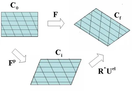
The single crystal model used in this work relies on an elastic-viscoplastic formulation. The main concepts are highlighted in this section and more details can be found elsewhere [Delannay et al., 2006]. In this model, plastic deformation is achieved by dislocation slip, along the {111} <110> crystallographic systems for FCC crystals deforming at low temperatures. The kinematics of the single crystal is a combination of dislocation slip, lattice rotation and elastic stretch. Figure 2.4 illustrates the multiplicative decomposition used in this work.
Fig. 2.4: Crystal kinematics: initial (C0), intermediate (Ci) and final configuration (Cf) The deformation gradient tensor F , typically considered in finite strain kinematics, is decomposed as follows:
F = FelFp =R∗UelFp, (2.20)
where Fp is the plastic deformation gradient that accounts for slip, R∗ is the lattice rotation
and Uel is the elastic stretch. The intermediate configuration C
i corresponds to a stress-free
configuration or “relaxed” configuration obtained by elastically unloading the crystal in the
fi-nal configuration Cf and rotating it. An additional fictitious configuration could be introduced
between Ci and Cf as in [Marin and Dawson, 1998b] where it is obtained by elastically
un-loading Cf to a relaxed state but without rotation. The crystal constitutive equations could be
to integrate them. In this work, the equations are written in the intermediate configuration Ci. The velocity gradient tensor L is given by:
L = ˙F F−1 = ˙R∗R∗T +R∗� ˙UelUel−1�R∗T +R∗Uel� ˙FpFp−1�Uel−1R∗T . (2.21)
The plastic velocity gradient Lp, accounting for dislocation slip, is then written as follows:
Lp = ˙FpFp−1 =� α
Mα˙γα. (2.22)
In this expression, Mα is the Schmid tensor of slip system α and ˙γα is the corresponding rate
of dislocation slip. The Schmid tensor has the same expression in the initial and intermediate configuration as crystallographic slip does not distort the lattice.
The elastic strain tensor E is calculated with respect to the intermediate configuration and is therefore given by:
E = 1 2 � FelTFel− 1�= 1 2 � UelTUel− 1� . (2.23)
The work-conjugate measure of stress is the second Piola-Kirchhoff stress T . This latter is related to the Cauchy stress σ through:
T =det(Fel)Fel−1σFel−T =det(Uel)Uel−1R∗TσR∗Uel−1 . (2.24)
The elasticity relation between T and E is given by:
T = CE , (2.25)
where C is a fourth order anisotropic elasticity operator. For cubic symmetry, the correspond-ing matrix has a form identical to the isotropic case, except that three independent constants are needed to fully describe the matrix [Hosford, 1993]. This form allows for the separation of the deviatoric and spherical components of T .
Infinitesimal elastic strains assumption
For materials subjected to important plastic strains, the elastic strains are small compared to plastic one. Typically, in metal forming operations, they never exceed 1%. It is then assumed that they are small compared to unity. This assumption yields:
Uel=1l + εεεel, (2.26)
where1l is the identity tensor, εεεelis a symmetric tensor with���εεεel���� 1. Neglecting higher order terms in εεεelleads to:
For the same sake of simplification, for any tensor X, εεεel : X is neglected compared to X. Bearing these assumptions in mind, the velocity gradient tensor can be rewritten as:
L = ˙R∗R∗T +R∗ ˙εεεel+ � α Mα˙γα R∗T , (2.27)
and equations 2.23,2.24 and 2.25 simplify to:
T = Cεεεel= R∗TσR∗. (2.28)
Flow rule and hardening model
In order to complete the single crystal model, the viscoplastic exponential law is used as a flow rule: ˙γα = ˙γ 0 �� �� �τ α τc �� �� � 1/m sign(τα) , (2.29)
where τα = T : Mα is the resolved shear stress, ˙γ
0 is a reference slip rate, m the sensitivity
exponent, and τc the critical resolved shear stress which is assumed to be identical for all slip
systems. A rate sensitive formulation is used here in order to avoid the non-uniqueness problem associated with the identification of the active slip systems in rate independent formulations.
Regarding the hardening, it is assumed that all slip systems have the same τcand that they
all harden equally according to the following rule: τc = τc0 � 1 + Γtot Γ0 �n with Γtot = � t 0 � α |˙γα| dt , (2.30)
where τc0, Γ0 and n are material parameters. Increase in slip resistance is therefore directly
related to the total shear accumulated on all slip systems. A Voce type saturation law is also implemented as follows: ˙τc =H0 � τsat− τc τsat− τ0 � � α |˙γα| , (2.31)
where τ0and τsatrepresent the initial and the saturation values of τcand H0a hardening
IV.2 Time integration scheme of the constitutive law
To summarize, the equations describing the elasto-viscoplatic model can be listed as fol-lows: Kinematics: Lsym → D = R∗ ˙εεεel+ � α 1 2(M α +MαT)˙γα R∗T , (2.32a) Kinematics: Lanti→ W = ˙R∗R∗ T +R∗ � α 1 2(M α− MαT)˙γα R∗T , (2.32b) Elasticity: T = Cεεεel, (2.32c) Schmid Law: τα= T : Mα, (2.32d) Flow: ˙γα = ˙γ0 �� �� � τα τc �� �� � 1/m sign(τα) , (2.32e) Hardening: τc = τc0 � 1 + Γtot Γ0 �n , Γtot = � t 0 � α |˙γα| dt . (2.32f)
The objective of the integration of the constitutive model is to compute the model-dependent variables at time t + ∆t, given that their values are known at time t and that the applied defor-mation is known for every crystal ( L or equivalently D and W ). In the previous system, the
unknown independent variables are: the crystal stresses T |t+∆t ( or equivalently the elastic
de-formation εεεel|
t+∆t), the slip resistance τc|t+∆t and the lattice orientation R∗|t+∆t. These constitute the state variables of the problem. In order to simplify the time integration procedure, one can choose to eliminate the lattice rotation from this system ( and hence the evolutionary equation
2.32b ) which is approximated by �R∗as follows:
R∗|t+∆t ≈ �R∗=W ∆tR∗|t .
As mentioned in [Delannay et al., 2006], the impact of such an approximation is negligible in metal forming simulations such as those performed in this work. The update of the lattice orientation is performed later, after the integration of the rest of the equations, as it is explained below.
Equations 2.32a, 2.32c and 2.32d are combined in order to find the crystal stresses T |t+∆t.
A fully implicit time integration scheme yields the following discretized equations: T|t+∆t = T|t +C � � R∗T∆D �R∗− 1 2(Mα+Mα T )∆γα � , (2.33a) ∆γα = ˙γα|t+∆t∆t = ˙γ0 � Mα : T | t+∆t τc|t+∆t �1/m sign(Mα : T | t+∆t)∆t , (2.33b) τc|t+∆t = τc0 � 1 + Γtot|t+∆t �n
with Γtot|t+∆t = Γtot|t+ �
on the stress estimate. Slip resistance is computed subsequently. Finally, regarding lattice reori-entation, equation 2.32b is integrated using an exponential map ([Simo and Hughes, 1998]). In
practice, all these equations are expressed in the crystal reference frame so that Mαis identical
in crystals belonging to the same phase. At the beginning of the simulation, the orientation of each grain is recorded and used to shift from the sample coordinate system to the crystal coor-dinate system (R0R∗T).
Link with the Finite Element formulation
The Cauchy stress, used by the finite element model, is updated according to 2.28, yield-ing:
σ|t+∆t = R∗T|t+∆tR∗
T
. (2.34)
Moreover, a consistent algorithmic tangent operator is used by the finite element formulation, as highlighted in the next chapter. It is given by:
C = ∂∆σ ∂∆D ≈ R ∗| t+∆tR�∗T ∂T|t+∆t ∂( �R∗T∆D �R∗)R� ∗R∗T| t+∆t, (2.35) where ∂T|t+∆t ∂( �R∗T∆D �R∗) = � C−1+� α 1 2(Mα+Mα T ) ⊗ ∂T∂∆γ| α t+∆t �−1 . (2.36)
This last equation is obtained by differentiating equation 2.33a with respect to the deformation increment. The last term in equation 2.36 is obtained from the solution of the following linear set: � α � δαβ+ ∆γα ∂mτc|t+∆t ∂τc|t+∆t ∂∆γβ � ∂∆γα ∂T|t+∆t = ∆γβ mMβ : T t+∆tM β, (2.37) where ∂τc|t+∆t ∂∆γβ = nτc0 � 1 + Γtot|t+∆t Γ0 �n−1 sign∆γβ Γ0 . (2.38)
The assessment of the time integration scheme can be found elsewhere [Delannay et al., 2006].
V Conclusion
As seen in this chapter, the behavior of a single crystal could be modelled in a more or less complex fashion so as to reflect the actual physical mechanisms operating at the microstruc-tural level. The slip system concept represents a homogenized way of taking into consideration the motion of individual dislocations that glide through the crystal lattice under the effect of the (resolved) stress. The flow rule reflects the non-linear relationship between strain rate and stress. It is phenomenological in nature, even if various authors have strived to incorporate more
“physics” into their models by, for example, considering dislocation densities as primary vari-ables, distinguishing the behavior of statistically stored dislocations from geometrically nec-essary ones, and therefore including strain gradients effects so as to account for non-local or long-range influences. Local models, such as the one used in this work, are blind to those in-fluences and, thus, do not include any length scale. They are, therefore, not expected to yield satisfactory results in several instances, including, for example, the prediction of the Hall-Petch effect, which is one of the most well-known macroscopic manifestation of size-related effects in metallic materials. Most importantly, they can not capture all grain scale heterogeneities, particularly those that appear under the influence of strain gradients. Bearing these limitations in mind, the single crystal model is in general combined with another model at the level of the polycrystal in order to account for the interaction between each grain and its neighbors. As-sumptions about grain interaction are as significant as the single crystal model in determining the outcome of the modelling effort, as seen in the following chapter.
Chapter 3
Accounting for grain interaction
Single crystals are in general part of a polycrystal and therefore, when this latter is sub-jected to loading, the behavior of each crystal (and that of the ensemble) is affected by the presence of the other constituents. The objective of polycrystal theories is to account for the individual behavior of the crystals and that of the polycrystal by defining:
• The way the deformation is partitioned among the crystals and the interaction between the grain and its neighbors,
• Whether or not the grain is considered as an homogeneous entity.
The CPFEM approach can be considered as being the ultimate polycrystal model. Its assump-tions regarding deformation and stress equilibrium are the closest to the actual physics of the problem compared to classical polycrystal models and more elaborate “N-site” models, as high-lighted in this chapter.
I Polycrystal theories
Polycrystal models are based on the Representative Volume Element (RVE) concept. The RVE polycrystal should be small enough compared to the macroscopic scale but large enough to reflect microstructural heterogeneities. In homogenization theory, the RVE is such as the loading and displacement conditions at its boundary are uniform and the volume average of
stress, strain and velocity gradient over all grains are equal to the overall stress Σpoly , strain
follows: Σpoly=�σc� = 1 V � Vσ cdV , Epoly=�εεεc� = 1 V � V εεεcdV , Lpoly=�Lc� = 1 V � VL cdV , (3.1)
where V is the volume of RVE, c stands for the crystal and poly for the polycrystal. Polycrystal models are basically composed of: (i) single crystal constitutive relations and (ii) a localization rule which is used to partition the macroscopic deformation among the grains (see figure 2.2). They are in essence statistical models. Several approaches, with their own variants, are present in the literature. Only the main ones are recalled here. These models are needed in Finite Ele-ment simulations where each integration point represents a group of crystals. They incorporate more or less complex assumptions in order to account for the interactions between the grains inside a polycrystal. After briefly discussing the earliest of them all, the Sachs model, the Tay-lor ( Full-Constraints) model is presented followed by classical TayTay-lor-Type models (Relaxed-Constraints) and more elaborate Taylor-Type models that strive to take into account the direct neighborhood of each grain by considering “clusters” of grains (N-site). While these models are based on short-range interactions, the Self-Consistent approach incorporates the long-range interactions between one cluster ( a grain or a group of grains) and the rest of the polycrystalline matrix.
I.1 Sachs model
In this model [Sachs, 1928] and its variants, grains are assumed to experience the same state of stress as the macroscopic polycrystal one and achieve deformation by activating only one slip system like unconstrained single crystals. No link or assumption is made about the deformation of each grain or the interaction between the grains. Therefore each grain deforms independently. While stress equilibrium is forced upon the system with the uniform stress assumption, compatible deformation is not achieved. This model is often presented as a “lower-bound”.
I.2 Taylor full-constraint model (FC)
Taylor’s original analysis [Taylor, 1938] is motivated by the violation of compatibility (or equivalently the assumption of single slip) in Sach’s model. Taylor assumed that all grains
![Fig. 2.3: 2D projection of yield surface in stress space (a) single slip representation; (b) multiple slip representation;(c) rate independent vs rate dependent plasticity [Kocks, 1998a]](https://thumb-eu.123doks.com/thumbv2/123doknet/2992279.83656/24.892.125.767.115.384/projection-surface-representation-multiple-representation-independent-dependent-plasticity.webp)