HAL Id: hal-00917847
https://hal-imt.archives-ouvertes.fr/hal-00917847
Submitted on 14 Dec 2013
HAL is a multi-disciplinary open access
archive for the deposit and dissemination of
sci-entific research documents, whether they are
pub-lished or not. The documents may come from
teaching and research institutions in France or
abroad, or from public or private research centers.
L’archive ouverte pluridisciplinaire HAL, est
destinée au dépôt et à la diffusion de documents
scientifiques de niveau recherche, publiés ou non,
émanant des établissements d’enseignement et de
recherche français ou étrangers, des laboratoires
publics ou privés.
A generic, robust and fully-automatic workflow for 3D
CT liver segmentation
Romane Gauriau, Rémi Cuingnet, Raphael Prevost, Benoit Mory, Roberto
Ardon, David Lesage, Isabelle Bloch
To cite this version:
Romane Gauriau, Rémi Cuingnet, Raphael Prevost, Benoit Mory, Roberto Ardon, et al.. A generic,
robust and fully-automatic workflow for 3D CT liver segmentation. MICCAI Workshop on Abdominal
Imaging, Sep 2013, Nagoya, Japan. pp.241-250. �hal-00917847�
A Generic, Robust and Fully-Automatic
Workflow for 3D CT Liver Segmentation
Romane Gauriau1,2, R´emi Cuingnet2, Raphael Prevost2, Benoit Mory2,
Roberto Ardon2, David Lesage2, and Isabelle Bloch1
1 Institut Mines-Telecom, Telecom ParisTech, CNRS LTCI, 46 rue Barrault,
75013 Paris, France
2 Philips Research MediSys, 33 rue de Verdun, 92156 Suresnes Cedex, France
Abstract. Liver segmentation in 3D CT images is a fundamental step for surgery planning and follow-up. Robustness, automation and speed are required to fulfill this task efficiently. We propose a fully-automatic workflow for liver segmentation built on state-of-the-art algorithmic com-ponents to meet these requirements. The liver is first localized using regression forests. A liver probability map is computed, followed by a global-to-local segmentation strategy using a template deformation framework. We evaluate our method on the SLIVER07 reference database and confirm its state-of-the-art results on a large, varied database of 268 CT volumes. This extensive validation demonstrates the robustness of our approach to variable fields of view, liver contrast, shape and patholo-gies. Our framework is an attractive tradeoff between robustness, ac-curacy (mean distance to ground truth of 1.7mm) and computational speed (46s). We also emphasize the genericity and relative simplicity of our framework, which requires very limited liver-specific tuning. Keywords: liver segmentation, fully-automatic segmentation, template deformation, regression forest, 3D CT
1
Introduction
Liver segmentation is required in many clinical contexts such as tumor resec-tion, follow-up or liver transplantation. It enables the computation of anatomical measures that are important for clinical diagnosis, surgery planning and radia-tion dose calcularadia-tion [1]. Manual liver segmentaradia-tion in 3D is both tedious and time-consuming and its automation is particularly challenging given the high variability of liver shapes, pathologies and contrast in different CT phases.
The literature on liver segmentation includes a large variety of interactive, semi-automatic and automatic methods. Due to space restrictions, we refer the reader to recent and extensive reviews [2,3] and to the SLIVER07 segmentation challenge [4,5] for more detailed bibliographic overviews. Those reviews highlight different groups of methods such as intensity-based, active contours, statistical shape models, graph-cuts and atlas-based registration. They also show that most segmentation methods focus on CT images with specific fields of view and partic-ular CT phases (often contrast-enhanced) which may restrict their clinical use.
Quantitative evaluation is another key point when comparing different methods. The challenge SLIVER07 [4] has become a reference for liver segmentation, en-abling fast and easy comparisons [5]. Unfortunately this database is limited to 20 training and 10 testing datasets. In the literature, only few methods were validated on extensive databases. One can cite [6,7,8], where the authors used proprietary databases composed of 277, 75 and 48 images respectively. However the differences in evaluation criteria and database composition make compar-isons of these methods difficult.
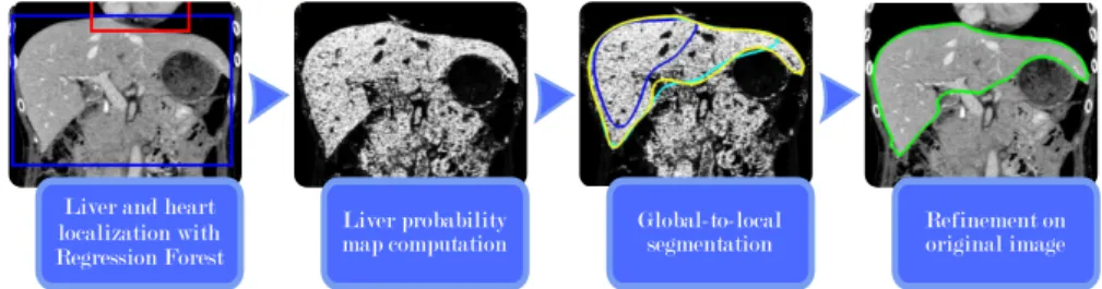
We propose a fully-automatic and robust method for the segmentation of the liver on CT data. Our workflow is inspired by [9], which proved its efficiency for CT kidney segmentation. Our method consists of four main parts built on state-of-the-art algorithmic components as shown in Fig. 1. The liver and the heart are first localized using regression forests [10] (see Section 2). We then compute a liver probability map based on intensity distributions (see Section 3). A template deformation framework [11] performs the liver segmentation using a global-to-local strategy (see Section 4.2). A final refinement step is applied using the original image.
In Section 5, we reuse and extend the validation framework of the SLIVER07 challenge and present a quantitative evaluation on both the SLIVER07 database and a large and diverse database (268 CT volumes with various fields of view, contrasts, liver shapes and pathologies). The results demonstrate, in an extensive and coherent fashion, the computational efficiency, robustness and accuracy of our method.
Liver and heart localization with Regression Forest
Liver probability
map computation Global-to-local segmentation Refinement on original image
Fig. 1: Workflow of our fully-automatic liver segmentation method.
2
Liver Localization Using Regression Forest
The authors of [10] recently demonstrated that regression forests are robust and memory efficient for the quick localization of multiple abdominal organs in 3D CT scans (1s/tree with their C++ implementation). They compared this method with the commonly used atlas-based method [12] and demonstrated that it is about a hundred times faster, uses ten times less memory and is more accurate.
The main idea behind regression forest is to use random forest for non-linear regression of multidimensional output given multidimensional input. Using training data, binary trees are built so as to split the data into clusters, in which the prediction can be achieved with a simple regression function.
As in [9], we use the regression forest method to detect bounding boxes of the liver and heart (see Fig. 1), each of them being parametrized with a vector of R6 composed of the coordinates of two extremal vertices. The training phase
is performed using random subsets of voxels of the training images. The features used are the same as in [10]: for each voxel we compute the mean intensities in two randomly displaced boxes. This exploits the fact that the intensities in CT images have a real physical meaning. In the testing phase a random selection of voxels votes for the predicted labels. A detailed and comprehensive description of the regression forests method can be found in [10].
This approach provides robust estimates of the positions and sizes of the liver and heart which are used to derive a liver probability map described hereafter.
3
Liver Probability Map Computation
Segmenting the liver directly in the image may provide insufficient results, in particular in images with poor contrast and fuzzy liver contours. Consequently, we propose to also take advantage of intensity distribution to pre-process the image and enhance liver voxels as shown in Fig. 2.
(a) (b) (c) (d)
Fig. 2:Probability map computation steps: (a) original image, (b)liver predicted box (blue), fitted mean liver (green), heart segmentation (pink), voxels patch
(yellow), probability map (c) before and (d) after heart masking.
3.1 Fitting a Mean Liver Model in the Predicted Bounding Box Mean liver computation A mean liver model is built using a set of manually segmented liver shapes, represented as meshes. We first register the shape meshes using the fast and robust registration method of [13]. The main interest of this method over the classical Iterative Closest Point approach [14] is to overcome the problem of point correspondence and to use a robust norm to obtain a consistent registration of the shapes. The mean liver model is obtained by averaging the implicit functions of the registered shapes.
Mean liver fitting The mean liver shape is scaled anisotropically so as to best fit the predicted bounding box of the liver.
3.2 Estimation of the Intensity Histogram
From the previously fitted mean liver model barycenter we select a cuboidal patch (∼ 603 mm3) of voxels, as illustrated in Fig. 2(b). The intensity histogram
is computed in this patch. Its normalization provides a function h : R → [0, 1] which gives an estimation of the probability of each intensity value to belong to the liver.
3.3 Coarse Segmentation of the Heart
In addition to the estimation of liver intensities, we roughly segment the heart in the image. This segmentation is performed on the original image with the template deformation framework described in Subsection 4.1. We initialize the algorithm with a mean heart model, built similarly to the mean liver shape and fitted in the predicted heart bounding box (see Subsection 3.1). Deformation parameters (see Table 1) are set so as to prevent the heart contour from leaking in the liver. Conversely the rough binary mask Mh we obtain will prevent the
liver contour from leaking in the heart in the subsequent steps.
3.4 Probability Map Computation
The liver probability map Ml: Ω → [0, 1] is defined as:
∀x ∈ Ω, Ml(x) = (1 − Mh(x)) h(I(x)) (1)
where Ω is the image domain and I is the image. A subsampling of the image can be previously applied to increase the computational efficiency.
This probability map (see Fig. 2 (d)) is used in subsequent segmentation steps.
4
Template-Based Global-to-Local Segmentation
We use the template deformation framework introduced in [11] to extract the liver contours from the probability map and the original image. Hereafter we briefly describe the model-based deformation algorithm we employ and detail the proposed global-to-local strategy to complete the segmentation.
4.1 Template Deformation Framework
The model-based approach of [11] is specially suited when target objects have partially unclear edges as the algorithm fairly extrapolates the contours. Key ad-vantages of the method are its speed, robustness and its ability to use both con-tour and region information. Let us present the main principles of this method.
Given an image J : Ω → R and an initial shape model represented by an implicit function φ : Ω → R, we look for the transformation ψ : Ω → Ω minimizing the following energy function:
Es(ψ) = α Z (φ◦ψ)−1(0) −h~∇J(x), ~n(x)idx | {z } flux term + (1 − α) Z (φ◦ψ)−1(R+) r(x)dx | {z } region term + λ R(ψ) | {z } regularization term (2) where
– α∈ [0, 1] is a constant defining the relative influence of flux and region terms (it enables to define whether we want to rely more on image contours or more on intensity contrast between regions);
– ~∇J(x) is the gradient of the image J in x and h . , . i is the scalar product; – ~n(x) is the normal vector to the shape at point x;
– r(x) is the region term defined as r(x) = logPint(J(x))
Pext(J(x)) where Pintand Pextare
the intensities distributions inside and outside the deformed object regularly estimated on the working image;
– R(ψ) prevents large deviations from the original shape model;
– λ∈ [0, 1] is a constant parameter tuning the strength of the shape constraint. In the general formulation the transformation ψ is decomposed as ψ = L ◦ G where G is a global linear transformation and L is a non-rigid local transfor-mation (refer to [11] for more details). Further we introduce Grand Gsdefining
a rigid and a similarity transformation, respectively. The regularization term is defined as R(ψ) = 1
2kL − Idk 2
2 where Id is the identity transformation.
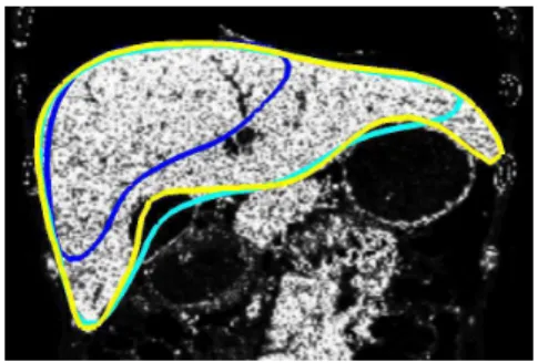
4.2 Global-to-Local Segmentation Workflow
Liver segmentation is performed according to an original global-to-local strategy on the probability map using the above-mentioned algorithm. Four steps help refining the contour progressively: 3 steps are performed on the probability map Ml and the final step on the original image I as shown on Fig. 3. Parameters
have been set experimentally and are kept identical in all processed examples (see Table 1). We observed a relatively low sensitivity to parameter variations in practice.
Step 1: Initialization The liver shape model is fitted to the predicted liver bounding box. As the template deformation method tends to favor expansion displacements, we scale down the model by a factor 0.7. Then a first step aims at globally registering the shape model without any local deformation. Equation 2 is minimized using the parameters reported in Table 1. The high weight on the region term constrains the shape inside the liver, thus facilitating expansion in subsequent deformation steps.
Table 1: Parameters used for global-to-local segmentation. J ψ α λ Heart I L ◦ Id 0.8 0.1 Liver step 1 Ml Id ◦ Gr 0.4 − step 2 Ml L ◦ Gs 0.8 0.03 step 3 Ml L ◦ Id 1 0.01
Fig. 3:The three segmentation steps on the probability map:step 1(blue),
step 2(cyan),step 3(yellow).
Step 2: Coarse segmentation We deform the previous result, still minimiz-ing Equation 2 but with different parameters (see Table 1) allowminimiz-ing some local deformations. The flux term is now more important than the region term so that the model contours match liver edges more accurately.
Step 3: Local deformation The third step helps refining the segmentation. Now we only optimize local deformations (see Table 1). The flux term is used alone in order to reach the contours. Releasing the shape constraint finally helps reaching stretched parts such as liver tips.
Step 4: Refinement on the original image To improve the accuracy of the final segmentation, we apply guided filtering [15] on the binary mask of the previous segmentation result, using the original image as guide. As detailed in [15], the guided filter acts as a fast, local matting/feathering refinement step enabling the final segmentation to better match the edges of the original image.
5
Experiments and Results
In this part we present experiments on two databases. The first one is SLIVER07 [4], which has become a reference for liver segmentation evaluation. Secondly we use a large database of 268 diverse CT volumes, further demonstrating the accuracy and robustness of the method. In those two experiments both the regression forest and the mean liver model are learned solely on the 20 training datasets of SLIVER07 (publicly available), for the sake of result reproducibility. Com-putational times are given for a C++ implementation on a machine with four 2.3GHz cores (Core i7-2820QM) and 8Go RAM.
5.1 Training
For mean liver model building and regression forests training, we use the 20 train-ing images of SLIVER07. Before regression forest traintrain-ing we do not pre-register
or normalize the images. The forest of 7 trees and 12 decision levels is learned after randomly selecting a subset of 40.000 voxels per image. The minimum node size is 50 and the training computational time is about 10 minutes.
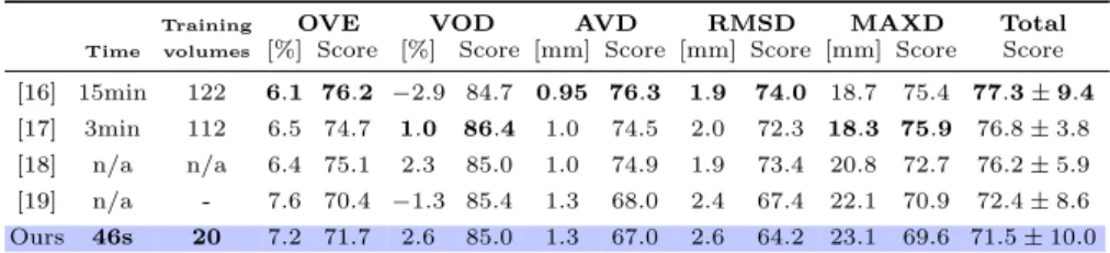
5.2 Evaluation on the SLIVER07 Database
We tested our method on the SLIVER07 challenge database [4] which is com-posed of 20 training and 10 testing 3D CT volumes (average slice and interslice resolution are 0.7mm±0.1 and 1.5mm±0.9, respectively) rather focused on the liver. The regression forest and mean liver shape were trained on the 20 training samples while we tested the algorithm on the 10 testing volumes. We compare our results with the best reported 3D methods [16,17,18,19] of the challenge, pointing the first three did not obtained those results in the challenge conditions (training on the 20 samples). Among these automatic methods ours comes in fifth position. In Table 2 we report the same validation measures (OVE: over-lap error, VOD: volume difference, AVD: average distance, RMSD: root mean squared distance, MAXD: maximum distance) and inter-observer scores (see [5]) as used in the challenge. Those results have also been published online [4].
Table 2: The five best automatic methods on SLIVER07 database. We report the computational time (per image), the number of training volumes and the SLIVER07 measures. (n/a: non available)
Training OVE VOD AVD RMSD MAXD Total
Time volumes [%] Score [%] Score [mm] Score [mm] Score [mm] Score Score
[16] 15min 122 6.1 76.2 −2.9 84.7 0.95 76.3 1.9 74.0 18.7 75.4 77.3 ± 9.4
[17] 3min 112 6.5 74.7 1.0 86.4 1.0 74.5 2.0 72.3 18.3 75.9 76.8 ± 3.8
[18] n/a n/a 6.4 75.1 2.3 85.0 1.0 74.9 1.9 73.4 20.8 72.7 76.2 ± 5.9
[19] n/a - 7.6 70.4 −1.3 85.4 1.3 68.0 2.4 67.4 22.1 70.9 72.4 ± 8.6
Ours 46s 20 7.2 71.7 2.6 85.0 1.3 67.0 2.6 64.2 23.1 69.6 71.5 ± 10.0
On this challenge database we get comparable results to best scored methods (see last column in Table 2). Our method also presents the advantage of being faster and requiring few samples for training. Moreover we thoroughly evaluate the robustness of liver localization in various conditions hereafter.
5.3 Evaluation on a Large Varied Database
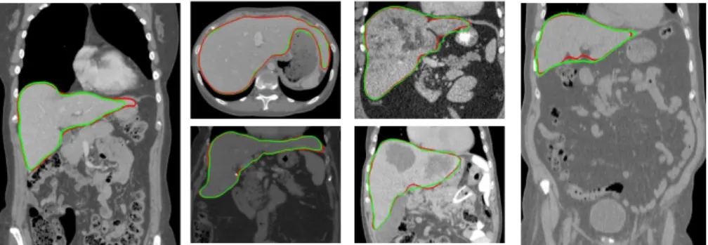
Database description The database we use in this experiment is composed of 268 3D CT images coming from 127 patients with diverse medical conditions (∼ 41% of patients with significant alterations of the liver shape and/or appear-ance). The database includes volumes with varied body shapes, fields of view (for 28% of the database the images include a large part of the trunk), resolution and use or no use of contrast agents (19% of delayed or non contrasted scans, 31%
of hepatic arterial phases and 50% of portal venous phases) as shown in Fig. 5. Slices and inter-slices resolution ranges from 0.5 to 1 mm and from 0.5 to 3 mm, respectively. The 268 images have been segmented manually by an expert.
The regression forest we use in this experiment is the same one as the one used previously. In Table 3 we report the results after each step thus showing the relevance of the global-to-local strategy. For the sake of consistency we use the same evaluation measures as in the first experiment. The localization with regression forest is fast (1.5s) and robust as the average distance (mean distance of box faces) is of 10.8mm for a maximum of 46.8mm. In comparison the authors of [10] obtain an average distance of 15.7mm for liver localization. We again emphasize that the regression forest was trained on only 20 datasets, which further highlights the robustness of the method.
Table 3: Results and computational time after each step of the algorithm re-ported as Mean ± Standard-Deviation.
Time OVE VOD AVD RMSD MAXD [sec.] [%] [%] [mm] [mm] [mm] RF localization 1.5 - - 10.8 ± 6.8 - -Proba. map 6 - - - - -Step 1 1 57.7 ± 10.4 57.3 ± 11.1 23.8 ± 9.9 31.6 ± 12.3 84.9 ± 27.4 Step 2 10 10.4 ± 6.7 −1.0 ± 6.0 2.3 ± 3.2 4.0 ± 4.6 23.3 ± 14.9 Step 3 23 9.6 ± 6.7 −2.4 ± 5.7 1.9 ± 2.9 3.3 ± 4.1 21.5 ± 13.7 Step 4 5 8.4 ± 6.7 −1.5 ± 5.6 1.7 ± 2.4 3.0 ± 3.6 21.7 ± 14.1
Overlap error (%)(a) (b) (c) -5
0 5 10 15
Vol. difference (%)(a) (b) (c) -5
0 5 10 15
Av. distance (mm)(a) (b) (c) 0 2 4 6 RMSD (mm) (a) (b) (c) 0 2 4 6
Max. distance (mm)(a) (b) (c) 10
20 30 40
Fig. 4: Boxplots for (a) step 2 (b) step 3 and (c) step 4. They represent 1st and 9th decile, 1st and 3rd quartile,median(dark-blue dash) andmean(pink cross).
After the last refinement we obtain mean and median distances of 1.7mm and 1.3mm, respectively. The median value highlights the presence of a limited number of outliers. Indeed for more than 90% of the database the overlap error is below 15.8% and the average distance below 3mm. Outliers can be principally
explained by a wrong initial position of the shape model (imprecise bounding box) and by diseases giving a very atypical appearance to the liver. In Fig. 4 we represent boxplots of the different measures, showing the relatively compact dis-persion of them. These results confirm those obtained on the SLIVER07 database and are good, despite the much larger variability of the database. Fig. 5 shows the segmentation accuracy in various situations.
Fig. 5: Examples of segmentation results (red:ground truth, green: our result) in varied situations: different fields of view, liver contrast, shape and pathologies.
6
Conclusion
In this paper we proposed a fully-automatic workflow for CT liver segmentation, robust to a large variety of imaging conditions: different fields of view, different CT phases, healthy and diseased livers. Our method relies on regression forests to predict liver and heart bounding boxes, computes a probability map from an estimation of the liver intensity distribution and uses a template-based deforma-tion algorithm to perform the liver segmentadeforma-tion in a global-to-local strategy.
Our state-of-the-art results on the SLIVER07 database are confirmed by an additional, extensive evaluation on a large and heterogeneous database (268 vol-umes). This validation demonstrates that our framework reaches an attractive balance between robustness, accuracy (mean distance to ground truth of 1.7mm) and speed (46s). We emphasize the genericity and relative simplicity of our framework, which required very limited liver-specific tuning. It is reproducible and could be improved in a number of ways. For instance, failed segmentations could be detected and easily corrected by the clinician as the template deforma-tion framework we employ can handle user interacdeforma-tions [11]. Finally we believe similar workflows could be applied to other organs and imaging modalities.
References
1. Murthy, R., Nunez, R., Szklaruk, J., Erwin, W., Madoff, D.C., Gupta, S., Ahrar, K., Wallace, M.J., Yttrium-90 microsphere therapy for hepatic malignancy: Devices,
indications, technical considerations, and potential complications. Radiographics 25(suppl 1), S41–S55 (2005)
2. Campadelli, P., Casiraghi, E., Esposito, A.: Liver segmentation from computed tomography scans: A survey and a new algorithm. Artificial Intelligence in Medicine 45(2-3), 185–196 (2009)
3. Mharib, A.M., Ramli, A.R., Mashohor, S., Mahmood, R.B.: Survey on liver CT image segmentation methods. Artificial Intelligence Review 37(2), 83–95 (2011) 4. Heimann, T., Styner, M., van Ginneken, B.: Sliver07. http://www.sliver07.org
(2007), accessed: 2013-05-12
5. Heimann, T., et al.: Comparison and evaluation of methods for liver segmentation from CT datasets. IEEE Transactions on Medical Imaging 28(8), 1251 –1265 (2009) 6. Ling, H., Zhou, S.K., Zheng, Y., Georgescu, B., Suehling, M., Comaniciu, D.: Hi-erarchical, learning-based automatic liver segmentation. In: Proc. CVPR’08. pp. 1–8 (2008)
7. Zhang, X., Tian, J., Deng, K., Wu, Y., Li, X.: Automatic liver segmentation using a statistical shape model with optimal surface detection. IEEE Transactions on Biomedical Engineering 57(10), 2622–2626 (2010)
8. Linguraru, M.G., Sandberg, J.K., Li, Z., Shah, F., Summers, R.M.: Automated segmentation and quantification of liver and spleen from CT images using normal-ized probabilistic atlases and enhancement estimation. Medical Physics 37(2), 771 (2010)
9. Cuingnet, R., Prevost, R., Lesage, D., Cohen, L., Mory, B., Ardon, R.: Automatic detection and segmentation of kidneys in 3d ct images using random forests. In: Ayache, N., Delingette, H., Golland, P., Mori, K. (eds.) Medical Image Computing and Computer-Assisted Intervention - MICCAI 2012, Lecture Notes in Computer Science, vol. 7512, pp. 66–74. Springer Berlin Heidelberg (2012)
10. Criminisi, A., Robertson, D., Konukoglu, E., Shotton, J., Pathak, S., White, S., Siddiqui, K.: Regression forests for efficient anatomy detection and localization in computed tomography scans. Medical Image Analysis (In press 2013)
11. Mory, B., Somphone, O., Prevost, R., Ardon, R.: Real-time 3d image segmen-tation by user-constrained template deformation. In: Ayache, N., Delingette, H., Golland, P., Mori, K. (eds.) Medical Image Computing and Computer-Assisted Intervention - MICCAI 2012, Lecture Notes in Computer Science, vol. 7510, pp. 561–568. Springer Berlin Heidelberg (2012)
12. Klein, S., Staring, M., Murphy, K., Viergever, M.A., Pluim, J.P.: Elastix: a tool-box for intensity-based medical image registration. IEEE Transactions on Medical Imaging 29, 196–205 (2010)
13. Fitzgibbon, A.W.: Robust registration of 2D and 3D point sets. Image and Vision Computing 21(13-14), 1145–1153 (2003)
14. Besl, P.J., McKay, N.D.: A method for registration of 3-d shapes. IEEE Transac-tions on Pattern Analaysis and Machine Intelligence 14(2), 239–256 (1992) 15. He, K., Sun, J., Tang, X.: Guided image filtering. In: Daniilidis, K., Maragos, P.,
Paragios, N. (eds.) Computer Vision - ECCV 2010, Lecture Notes in Computer Science, vol. 6311, pp. 1–14. Springer Berlin Heidelberg (2010)
16. Kainm¨uller, D., Lange, T., Lamecker, H.: Shape constrained automatic segmenta-tion of the liver based on a heuristic intensity model. In: Proc. MICCAI Workshop 3D Segmentation in the Clinic: A Grand Challenge. pp. 109–116 (2007)
17. Wimmer, A., Soza, G., Hornegger, J.: A generic probabilistic active shape model for organ segmentation. In: Yang, G.Z., Hawkes, D., Rueckert, D., Noble, A., Taylor, C. (eds.) Medical Image Computing and Computer-Assisted Intervention - MICCAI
2009, Lecture Notes in Computer Science, vol. 5762, pp. 26–33. Springer Berlin Heidelberg (2009)
18. Linguraru, M., Richbourg, W., Watt, J., Pamulapati, V., Summers, R.: Liver and tumor segmentation and analysis from ct of diseased patients via a generic affine invariant shape parameterization and graph cuts. In: Yoshida, H., Sakas, G., Lin-guraru, M. (eds.) Abdominal Imaging. Computational and Clinical Applications, Lecture Notes in Computer Science, vol. 7029, pp. 198–206. Springer Berlin Hei-delberg (2012)
19. Huang, C., Jia, F., Li, Y., Zhang, X., Luo, H., Fang, C., Fan, Y.: Fully automatic liver segmentation using probability atlas registration. In: International Conference on Electronics, Communications and Control 2012. pp. 126–129 (2012)