1 1
On the mixture of wind speed distribution in a Nordic region
23
4
Taha B.M.J. Ouarda1,*, Christian Charron1
5
6
7
1
Canada Research Chair in Statistical Hydro-Climatology, INRS-ETE, 490 de la Couronne,
8
Québec, QC, G1K 9A9, Canada
9 10 11 12 13 14 15 16 April 2018 17
2 Abstract
18
The assessment of wind energy potential at sites of interest requires reliable estimates of the
19
statistical characteristics of wind speed. A probability density function (pdf) is usually fitted to
20
short-term observed local wind speed data. It is common for wind speed data to present bimodal
21
distributions for which conventional one-component pdfs are not appropriate. Mixture
22
distributions represent an appropriate alternative to model such wind speed data. Homogeneous
23
mixture distributions remain rarely used in the field of wind energy assessment while
24
heterogeneous mixture models have only been developed recently. The present work aims to
25
investigate the potential of homogeneous and heterogeneous mixture distributions to model wind
26
speed data in a northern environment. A total of ten two-component mixture models including
27
mixtures of gamma, Weibull, Gumbel and truncated normal are evaluated in the present study.
28
The estimation of the parameter of the mixture models are obtained with the least-squares (LS)
29
and the maximum likelihood (ML) methods. The optimization of the objective functions related
30
to these estimation methods is carried out with a genetic algorithm that is more adapted to
31
mixture distributions. The case study of the province of Québec (Canada), a Northern region
32
with an enormous potential for wind energy production, is investigated in the present work. A
33
total of 83 stations with long data records and providing a good coverage of the territory of the
34
province are selected. To identify the most appropriate one-component distribution for the
35
selected stations, the newly proposed method of L-moment ratio diagram (MRD) is used. The
36
advantages of this approach are that it is simple to apply and it allows an easy comparison of the
37
fit of several pdfs for several stations on a single diagram. One-component distributions are
38
compared with the selected mixture distributions based on model selection criteria. Results show
39
that mixture distributions often provide better fit than conventional one-component distributions
3
for the study area. It was also observed that the ML method outperforms the LS method and that
41
the mixture model combining two Gumbel distributions using ML is the overall best model.
42
Keywords: wind speed distribution; moment ratio diagram; homogeneous mixture distribution; 43
heterogeneous mixture distribution; probability density function; model selection criteria; kappa
44
distribution.
4 Nomenclature
46
pdf probability density function
47
cdf cumulative distribution function
48
( )
f probability density function
49
i
P cumulative empirical probability for the ith wind speed class interval
50
i
p relative frequency for the ith wind speed class interval
51
ˆ
i
F estimated cumulative probability for the ith wind speed class interval
52
( )
F cumulative distribution function
53
1
( )
F inverse of a given cumulative distribution function
54
ω mixing weight in two-component mixture distributions
55
θ distribution parameters vector
56
W Weibull probability distribution
57
E Gumbel or extreme value type I probability distribution
58
G gamma probability distribution
59
GEV generalized extreme value probability distribution
60
GG generalized gamma probability distribution
61
KAP kappa probability distribution
62
LN lognormal distribution
63
P3 Pearson type III distribution
64 ML maximum likelihood 65 MM method of moments 66 LS method of least-square 67
MWW mixture of two 2-parameter Weibull
68
MWTN mixture of Weibull and singly truncated from below normal
69
MGW mixture of gamma and Weibull
70
MGG mixture of two gamma
71
MGTN mixture of gamma and singly truncated from below normal
72
MGE mixture of gamma and Gumbel
73
MEE mixture of Gumbel and Gumbel
5
METN mixture of Gumbel and singly truncated from below normal
75
MTNTN mixture of two singly truncated from below normal
76
n number of wind speed observations in a series of wind speed observations
77
N number of class intervals
78 2 p
R coefficient of determination giving the degree of fit between the estimated relative
79
frequencies of the theoretical pdf and the empirical relative frequencies of the
80
histogram of wind speed.
81 2 F
R coefficient of determination giving the degree of fit between the theoretical cdf
82
and the empirical cumulative probabilities of the histogram of wind speed.
83
RMSE root mean square error of the predicted relative frequencies
84
KS Kolmogorov-Smirnov test statistic
85 2
Chi-square test statistic
86
v wind speed
87
, , p r s
M probability weighted moment of order p, r, s
88 1 r rth L-moment 89 1 r rth sample L-moment 90 r rth L-moment ratio 91 r
t rth sample L-moments ratio
92
r
rth probability weighted moment where M1,r,0
93 r b unbiased estimator of B r 94 95 96
6 1. Introduction
97
The assessment of wind energy potential at sites of interest requires the estimation of the
98
distribution of observed local wind speed data. For this purpose, a probability density function
99
(pdf) is usually fit to short-term wind speed data (typically 1 hour). Selecting a PDF that
100
correctly characterizes the wind speed distribution is crucial for reducing uncertainties in wind
101
energy production estimates. The Weibull (W) is the most widely used and accepted distribution
102
for the estimation of wind energy potential (Archer and Jacobson, 2003; Celik, 2003; Akpinar
103
and Akpinar, 2005; Ahmed Shata and Hanitsch, 2006; Acker et al., 2007; Ayodele et al., 2012;
104
Irwanto et al., 2014; Petković et al., 2014; Carrasco-Díaz et al., 2015; Dabbaghiyan et al., 2016;
105
Yip et al., 2016). Its popularity can be attributed to its flexibility, simplicity and the fact that its
106
parameters are easy to estimate (Tuller and Brett, 1983). However, W does not allow describing
107
all encountered wind regimes in nature (Carta et al., 2008; Ouarda et al., 2015).
108
Several other distributions have been proposed in the literature for the assessment of wind
109
energy: the gamma (G), generalized gamma (GG), inverse gamma (IG), inverse gaussian (IGA),
110
lognormal (LN), logistic (L), log-logistic (LL), Gumbel (E), generalized extreme value (GEV),
111
three-parameter beta (B), Pearson type III (P3), log-Pearson type III (LP3), Burr (BR), Erlang
112
(ER), Johnson SB, kappa (KAP) and Wakeby (WA) (Carta et al., 2009; Zhou et al., 2010; Lo
113
Brano et al., 2011; Morgan et al., 2011; Masseran et al., 2012; Soukissian, 2013; Jung et al.,
114
2017).
115
The identification of the statistical model that provides the best fit to the data represents a
116
challenge. Traditionally, the fit was assessed using goodness-of-fit statistics and histograms of
117
observed wind speed plotted together with candidate theoretical distributions. Recently, Ouarda
7
et al. (2016) proposed the method of moment ratio diagram (MRD) for the selection of
119
theoretical distributions. MRDs are commonly used in a number of fields for distribution
120
assessment and parameter estimation (El Adlouni and Ouarda, 2007; Seckin et al., 2011), but
121
were never applied to wind speed modeling.
122
With this approach, all possible values of the standardized kurtosis and the standardized
123
skewness of the candidate distributions are usually plotted on a same graph. The sample
124
moments of the observed data at the stations of interest are then estimated from the observations
125
and plotted on the same graph. The selection of the appropriate distribution to fit the data sample
126
is made based on the position of the sample moments in the graph. The advantage of using this
127
approach is that it allows an easy comparison of the fit of several pdfs on a single graph. The
128
approach allows also the analysis of the fit of data from several stations on the same graph.
129
Hosking (1990) introduced the MRD using L-moment ratios instead of the conventional moment
130
ratios. The theoretical advantages of L-moments over conventional moments are that they are
131
able to characterize a wider range of distributions, they are more robust to the presence of
132
outliers in the data when estimated from a sample, and are less subject to bias in the estimation
133
(Hosking and Wallis, 1997). Ouarda et al. (2016) applied conventional MRD and L-moment
134
MRD to wind speed data and concluded that L-moment MRD provide results that are more
135
coherent with goodness-of-fit statistics and should be preferred over the conventional MRD. This
136
conclusion was also obtained in other studies dealing with hydrologic data (Hosking, 1990; El
137
Adlouni and Ouarda, 2007).
138
It has been shown in several studies that it is frequent for wind speed data to present
139
distributions with bimodal regimes (Jaramillo and Borja, 2004; Shin et al., 2016; Soukissian and
140
Karathanasi, 2017; Jung and Schindler, 2017; Mazzeo et al., 2018). In these cases, conventional
8
pdfs are not suitable for modelling such distributions. To cope with such regimes, mixture
142
distributions, defined as linear combinations of different distributions, were proposed by a
143
number of authors (Carta et al., 2009; Ouarda et al., 2015; Shin et al., 2016). Proposed mixture
144
models in the literature include mixtures of two Weibull distributions (Carta and Ramirez, 2007;
145
Akpinar and Akpinar, 2009), two normal distributions (Jaramillo and Borja, 2004), singly
146
truncated normal and Weibull distributions (Carta and Ramirez, 2007; Akpinar and Akpinar,
147
2009), two singly truncated normal distributions (Mazzeo et al., 2018; Chang, 2011), gamma and
148
Weibull (Chang, 2011), Weibull and Gumbel distributions (Shin et al., 2016) and singly
149
truncated normal and GEV distributions (Kollu et al., 2012). Homogeneous (the two components
150
represent the same distribution) and heterogeneous (the two components represent two different
151
distributions) mixture models are flexible and can provide good fit to bimodal regimes as well as
152
unimodal regimes (Carta and Ramirez, 2007; Shin et al., 2016). Their use is gaining increasing
153
popularity in the field of wind energy assessment and modeling.
154
Wind energy assessment and mapping studies remain relatively limited in Nordic
155
environments. The case study of the province of Québec, Canada, is used in the present work to
156
evaluate the suitability of homogeneous and heterogeneous mixture distributions for fitting wind
157
speed data. Ten different mixture distribution models mixing W, G, E and truncated Normal are
158
fitted to the wind speed at the stations of the study area. The choice of distribution functions used
159
in mixture models is based on previous studies (e.g. Shin et al., 2016) as well as the asymptotic
160
behavior of the tails of the distributions considered (El Adlouni et al., 2008), although the focus
161
is not only on extreme wind speeds for energy generation. A large number of meteorological
162
stations distributed all across the province are used for this objective. The province of Québec
163
represents a region with an enormous undeveloped potential for wind energy production. A very
9
limited number of studies evaluated the potential for wind energy in the province of Québec. In
165
all these studies, only W was used (Ilinca et al., 2003; HE&AWS, 2005) except for a limited
166
scope study where only two stations were explored (Ouarda and Charron, 2018). The method of
167
the L-moment ratio diagram is also applied for evaluating the adequacy to the data of a selection
168
of one-component distributions commonly used to model wind speed data. Note that, in their
169
current state, MRD cannot be used to represent mixture distributions and thus, only
one-170
component distributions are represented in these diagrams. Two-component homogenous and
171
heterogeneous mixture distribution functions combining G, E, singly truncated normal (TN) and
172
W as well as one-component W and KAP were fitted to the wind speed data of the study area.
173
Validation of goodness-of-fit was made using criteria commonly used in the field of wind energy
174
assessment. The results of the analysis are illustrated for a selection of 10 stations representing
175
the study area. These stations provide a good illustration of the range of behaviors of wind speed
176
distributions in the province of Québec.
177
The paper is organized as follows: Section 2 presents the theoretical background on
L-178
moment ratio diagrams, one component probability distributions and mixture models. Section 3
179
presents the methodology of the study, including the representation of pdfs in MRDs, the
180
estimation of distribution parameters and the model evaluation criteria. The case study dealing
181
with wind speed data in the province of Quebec is presented in Section 4. The results are
182
presented in Section 5, and the conclusions and future research directions are finally discussed in
183
section 6 of the paper.
184
185
2. Theoretical background 186
10
2.1. L-moment ratio diagrams
187
L-moments introduced by Hosking (1990) represent an alternative to the conventional
188
moments for the characterization of the shapes of probability distributions. The advantages of
L-189
moments over conventional moments are that they are able to characterize a wider range of
190
distributions, are more robust to the presence of outliers in the data and are less subject to bias in
191
estimation (Hosking, 1990). For a given random variable X with a cumulative distribution
192
functionF X( ), the probability weighted moments (PWMs) are defined by (Greenwood et al.,
193 1979): 194 , , E[ { ( )} {1 ( ) }] p r s p r s M X F X F X . (1) 195
A useful special case of the PWM used in the definition of L-moments is given by:
196 1 1, ,0 E[ { ( )} ] 0 ( ) r r r M r X F X x u u du
(2) 197where ( )x u is the quantile function of X. The L-moments of X are defined by (Hosking, 1990):
198 1 , 0 r r r k k k p
, r0,1, 2,... (3) 199 where 200 * , ( 1) r k r k r r k p k k . (4) 201L-moments are directly interpretable as measures of the shape of distributions. The
202
dimensionless versions of the L-moments, the L-variation, L-skewness and L-kurtosis, are
203
respectively given by:
11 2 2 1 3 3 2 4 4 2 / / / . (5) 205
An important property makes the L-moments especially useful for the assessment of the
206
goodness-of-fit with MRD: if the mean of the distribution exists, then all L-moments exist and
207
the L-moments uniquely define the distribution (Hosking, 1997). L-moment ratios 4 vs. 3 in 208
Eq. (5) are usually plotted in MRD for the assessment of the goodness-of-fit. A distribution
209
function with one shape parameter, two shape parameters, or three or more shape parameters, is
210
respectively represented as a point, a curve or an area in the MRD. The pdfs that are represented
211
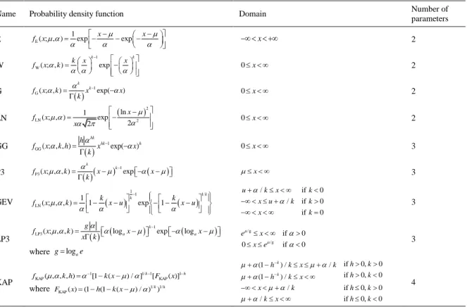
on the MRD of this study are given in Table 1 with their domain and number of parameters.
212
For a given data sample, the estimated values of the L-moment ratios can be obtained.
213
Sample L-moment ratios are then plotted on the MRD to evaluate the adequacy of the pdfs
214
represented in the MRD to the data samples. For an ordered sample of size n, x1x2 xn,
215
the sample L-moments are defined by:
216 1 , 0 , 0,1,..., 1 r r r k k k p b r n
(6) 217 where 218 1 1 1 1 n 1 r j j r n j b n x r r
. (7) 219The sample L-moment ratios analogous to the L-moment ratios in Eq. (5) are defined by:
12 2 2 1 3 3 2 4 4 2 / / / t t t . (8) 221
2.2. One-component probability distributions
222
In this study, the whole range of distributions commonly considered in wind energy
223
assessment and modeling were examined using MRD. The one-component W and KAP were
224
identified as the only one-component probability distributions which provide a good fit to the
225
wind speed data. Their pdfs were fitted to the wind speed data of the case study. W is the most
226
used and recognized pdf for analysis of wind speed data. The pdf of W is given by:
227
1 W exp k k k x x f x (9) 228where x0, 0 is a scale parameter and k is a shape parameter. The cumulative distribution
229
function (cdf) of W is given by:
230
W 1 exp k x F x . (10) 231KAP, introduced by Hosking (1994) is a four-parameter distribution that includes the generalized
232
logistic, the GEV, and the generalized Pareto distributions as special case. KAP was shown to
233
lead to very good fit to wind speed data in previous studies (Shin et al., 2016; Jung et al., 2017).
234
The pdf of the KAP is given by:
235 1 1/ 1 1 KAP( ; , , , ) [1 ( ) / ] [ KAP( )] k h f x k h k x F x (11) 236
and the cdf of KAP is given by:
13 1/ 1/ KAP( ; , , , ) (1 (1 ( ) / ) ) k h F x k h h k x (12) 238
where is a location parameter, is a scale parameter, h and k are shape parameters.
239
2.3 Singly truncated from below distributions
240
The singly truncated from below normal (TN) distribution is often adopted instead of the
241
conventional normal distribution in models for wind speed data (Carta et al., 2009). The reason is
242
that N allows negative values of wind speed which is not possible. Truncated distributions are
243
used to restrict the domain of the distributions. The truncation of the tails of the distribution was
244
also shown in previous studies to be robust to extreme observations in the sample and to lead to
245
improved estimates of the distribution moments, parameters and quantiles (see for instance Ouarda
246
and Ashkar, 1998). In the context wind speed modeling, the restriction x0 is applied. TN has
247
also the advantage over W of been able to represent calm frequencies as it is defined for x0.
248
However, adding a constraint to the Normal support makes the inference more complex when
249
other distributions are considered. If F xN( ; , ) and fN( ; , )x are the cdf and pdf of the
250
normal distribution, the pdf and cdf of the TN are defined by:
251 TN N 0 1 ( ; , ) ( ; , ) ( , ) f x f x I , (13) 252 N N TN 0 N 0 0 ( ; , ) (0; , ) 1 ( ; , ) ( ; , ) ( , ) ( , ) x F x F F x f x I I
(14) 253where x0 and the function 0 N N
0
( , ) ( ; , ) 1 (0; , )
I
f x F ensures that the integral254
of the pdf of TN is equal to one. Similarly, the truncated pdf and cdf of E can also be obtained by
255
using Eq. (13) and (14) and replacing fN( ; , )x by fE( ; , )x . 256
14
2.4. Mixture probability distributions
257
Mixture distributions are defined as linear combinations of two or several distributions.
258
For a mixed distribution with d components, the pdf is given by:
259 1 ( ; , ) ( ; ) d i i i i f v f v
. (15) 260where i are the parameters of the ith distribution, f vi( ; )i are independently distributed ith
261
components and ωi are mixing parameters such that
1 1 d i i
. In the case of a two-component262
mixture distribution, the mixture density function is then:
263
1 2 1 1 2 2
( ; , , ) ( ; ) (1 ) ( ; )
f v f v f v . (16)
264
where 0 1 is the mixing weight, and 1 and 2 are vectors of parameters for the first and
265
second component of the distribution.
266
Similarly to the previous study of Shin et al. (2016), the G, W, E, and TN distributions
267
were adopted as density components of mixture distributions. In all, 10 mixture distributions are
268
obtained with the combination of the different components considered and are denoted by:
269
MGW, MGE, MGTN, MWW, MWE, MWTN, MEE, MEN and MTNTN. The pdfs of these
270
mixture models are presented in Table 2.
271 272 3. Methodology 273 3.1. Representation of the pdfs in MRD 274
15
In this section we explain how selected pdfs in Table 1 are represented in the MRD. The
275
distribution E, having no shape parameter, is defined by a dot on the MRD. Distributions E,
276
GEV, W, P3 and G have a single shape parameter, and plot as a line in the MRD. For the
277
previous distributions, polynomial approximations of 4 as function of 3 are available in
278
Hosking and Wallis (1997) and are used to plot the lines corresponding to these distributions in
279
the MRD. Distributions GG, LP3 and KAP having two shape parameters define areas in the
280
MRD and bounds of these areas are represented in the MRD. Analytical expressions of these
281
bounds are generally not available. In that case, the following numerical method is applied: For a
282
given pdf with two shape parameters h and k, a position parameter μ and/or a scale parameter α,
283
parameters h and k are varied over a large range within the feasibility domain of the given pdf
284
and with small intervals (hh h1, 2, ,h kn; k k1, 2, ,km). Parameters μ and α are given
285
arbitrary values because they are independent of L-moment ratios 3 and 4. For each generated
286
pair of values (h ki, j), the corresponding pairs of moment ratios (3, ,i j,4, ,i j) are computed and
287
are plotted on the L-moment ratio diagram. Afterwards, the contours of the regions defined by
288
these points are defined.
289
For KAP, the expressions of L-moment ratios 3 and 4 as a function of its distribution
290
parameters are given in Hosking and Wallis (1997). Explicit expressions of L-moments as a
291
function of the distribution parameters of the GG and LP3 are not available. In this case, B , 1 B 2
292
and B are estimated by numerically integrating the distribution in Eq. (2) and 3 2 3 and 4 are
293
obtained using Eq. (5).
294
3.2. Parameter estimation
16
Parameters of the W are estimated in the present work with the method of moments
296
(MM). Parameters of KAP are estimated here with the method of L-moments (Hosking, 1997).
297
Algorithm for this method can be found in Hosking (1996).
298
The parameters of the mixture distributions are commonly estimated with the least-square
299
(LS) method (Carta and Ramirez, 2007; Shin et al., 2016; Jung and Schindler, 2017) and the
300
maximum likelihood (ML) method (Carta et al., 2009; Shin et al., 2016). The least-squares are
301 defined by: 302 2 max, 1 ( | ) N i i i SSE P F v
(17) 303where P is the cumulative empirical probability of the ith group, i vmax,i is the maximum wind
304
speed of the ith group and is a parameter vector. Observed wind speed data are arranged into
305
N class intervals [0, ),[ ,v1 v v1 2),...,[vN1,vN]. Relative frequencies p are computed for each class i
306 interval and 1 i i j j P p
is the cumulative empirical probability at the ith class.307
The maximum likelihood method was applied on observed wind speeds. It is proposed
308
here to use the maximum likelihood with the class interval approach. Given an underlying
309
distribution ( ; )f x for the wind speed, the likelihood is given by (Carter et al., 1971):
310 1 ( ) i N n i i L C p
(18) 311 where 1 ! N i! iCn
n and n is the number of observations in the ith class interval. It is i312
generally more convenient to optimize the log-likelihood given by:
17
1
log ( ) log( ) log
N i i i L C n p
. (19) 314To optimize the least-squares function in Eq. (17) and the log-likelihood function in Eq.
315
(19), a genetic algorithm (GA) is used. GA has been used in different fields for the optimization
316
of a given objective function (Hassanzadeh et al., 2011). A particularity of GA which makes it
317
attractive for solving the problem associated to the estimation of the parameters of mixture
318
distributions is that it does not require defining initial values for the parameters, which is difficult
319
in the case of mixture distributions (Ouarda et al., 2015).
320
The approaches presented here for parameter estimation are sensitive to the discretization
321
interval selection. The intervals should have small extent but also contain enough observations,
322
which is not possible especially for small sample sizes. The choice of intervals depends also on
323
the sensitivity of the anemometer. For less precise anemometers, it is not possible to use very
324
fine intervals.
325
3.3. Validation
326
The chi-square test statistic (2), the coefficient of determination (R2), the RMSE and
327
the Kolmogorov-Smirnov test statistic (KS) are used for the validation of the goodness-of-fit of
328
the different models. These criteria are frequently used for the evaluation of the goodness-of-fit
329
(Ouarda et al., 2016). Before the computation of the statistics, wind speed data are arranged in N
330
class intervals and relative frequencies p are computed at each class interval. i
331
Two indices are used to define R2. The first index is defined by:
18 2 2 1 2 1 ˆ ( ) 1 ( ) N i j i F N i i P F R P P
(20) 333where Fˆi is the predicted cumulative probability of the theoretical distribution at the ith class
334 interval, 1 i i j j P p
is the empirical cumulative probability at the ith class interval and335 1 1 N i i P P N
. The second index is defined by:336 2 2 1 2 1 ˆ ( ) 1 ( ) N i i i p N i i p p R p p
(21) 337where pˆi F v( )i F v( i1) is the estimated probability at the ith class interval, vi1 and v are the i
338
lower and upper limits of the ith class interval and
1 1 N i i p p N
. 339The RMSE is a measure of the error in the estimation of the relative frequencies and is
340 given by: 341 1/2 2 1 ˆ RMSE N ( i i) / i p p N
. (22) 342The 2 test statistic is a measure the adequacy of a given theoretical distribution to a data
343
sample and is expressed as:
344
2 2 1 N i i i i O E E
(23) 34519
where O is the observed frequency in the ith class interval and i E is the expected frequency in i
346
the ith class interval. When E for a given class interval is very small, it is combined with the i
347
adjacent class interval in order to avoid the situation where E has an excessive weight. The KS i
348
statistic corresponds to the largest difference between the predicted and the observed distribution
349
and is given by:
350 1 ˆ max i i i N D P F . (24) 351
A lower value of 2, RMSE or KS, and a higher value of R2 indicate a better fit.
352
353
4. Nordic environment case study 354
4.1. Region of study
355
The province of Quebec (Canada) covers a territory of over 1.5 million km2 and has an
356
enormous potential for wind energy production. In a study commended by the government of
357
Quebec, it was concluded that the exploitable potential in Quebec is close to 4 000 000 MW
358
(HE&AWS, 2005). The majority of energy production in Quebec comes traditionally from
359
hydroelectricity (Barbet et al., 2006). Because of the large existing and potential hydroelectric
360
resources, the development of other renewable sources of energy has been considerably delayed.
361
Nevertheless, an increasing interest for renewable energy and especially for wind energy
362
harvesting is observed recently. The government of Quebec requested in its new energy policy to
363
support the development of new wind farm projects on the territory (Gouvernement du Québec,
20
2016). Wind generation is nowadays considered as a viable alternative for energy supply in
365
remote rural areas, especially in the Northern regions.
366
A very limited number of studies dealt with modeling wind speed and assessing the wind
367
energy resources in the province of Quebec (Ilinca et al., 2003; HE&AWS, 2005; Hundecha et
368
al., 2008). Ilinca et al. (2003) and HE&AWS (2005) evaluated the potential for wind energy in
369
the province based solely on the W distribution. Hundecha et al. (2008) studied the changes in
370
the annual maximum 10-m wind speed in and around the Gulf of St. Lawrence, Canada, through
371
a nonstationary extreme value analysis. The study was based on the North American Regional
372
Reanalysis (NARR) dataset as well as observed data from a selection of stations located on and
373
around the Gulf of St. Lawrence.
374
4.2. Wind speed data
375
The wind speed data used in this study were obtained from “Environment and Climate
376
Change Canada”, the Federal ministry of the Environment. Meteorological data are available
377
freely at http://climate.weather.gc.ca. Observed data consist of mean hourly wind speeds
378
observed at 10 m above the ground for meteorological stations distributed across the province of
379
Quebec. Stations with identical coordinates were combined together. Stations of the database
380
with at least one complete year of data were selected. A total of 83 stations covering most of the
381
territory of the province of Québec were selected. The geographical location of the selected
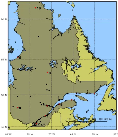
382
stations is illustrated in Fig. 1. The majority of the stations are located in the southern part of the
383
province of Quebec on both sides of the Saint-Lawrence River. The network density is
384
significantly higher in the southern part of the province due to the concentration of major urban
385
agglomerations and economic activities in this region.
21
The lengths of the data series at the stations range from 1 to 65 years with a median of 21
387
years of data. The calm frequencies at the stations are very low. 10 stations having long data
388
series and a good distribution across the study area were selected to illustrate the results of the
389
present study. These stations are considered representative of the whole data base. A detailed
390
description of the selected stations is presented in Table 3 with information concerning the
391
period of record, the geographical location and the statistical characteristics of the wind speed
392
data. The selected 10 stations are illustrated in the map of Fig. 1 with red dots. The rest of the
393
stations are illustrated with black dots.
394
395
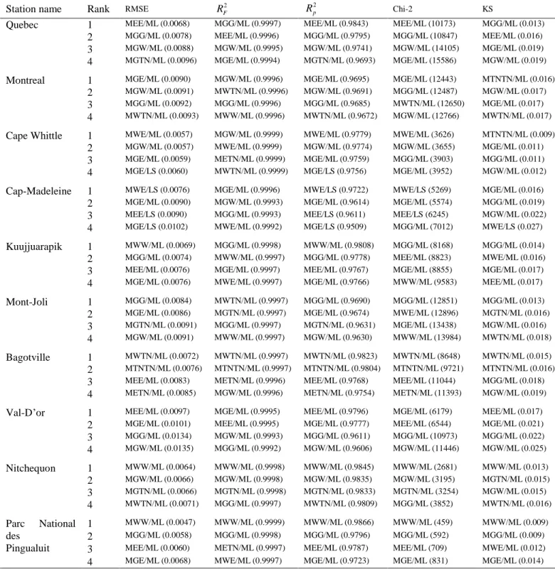
5. Results 396
Fig. 2 presents the L-moment ratio diagram with the selected one-component pdfs. KAP,
397
covering the largest area in the MRD, is thus the most flexible pdf, followed by LP3 and GG.
398
The GEV, W, G, P3 and LN, plot as lines and are similar for values of 3 around the zero value.
399
E is a special case of the GEV. The distributions G, P3 and W are special cases of the GG, and
400
the distributions GEV and E are special cases of the KAP distribution. Sample L-moments were
401
computed using Eq. (8) and (6) for each station of the study area and were plotted on the MRD.
402
It can be observed in Fig. 2 that the curve defined by W passes through the cloud of points
403
defined by the sample L-moment ratios. For the other distributions defining a curve (G, P3, GEV
404
and LN), the lines are located over the cloud of points and the distributions are thus inadequate
405
for representing wind speed data at the stations of the case study. It can hence be concluded that
406
W is the most suitable pdf with one shape parameter.
22
All 83 stations are located within the regions that are bounded by the pdfs of the
408
distributions possessing two shape parameters (GG, LP3 and KAP), and thus, these pdfs can
409
represent appropriate models for the wind speed data of the Quebec stations. Even though on
410
average W represents a good model, it may not be suitable for data sets located far from the
411
curve defined by W. In these cases, GG, LP3 and KAP provide a better fit and are more
412
appropriate.
413
MRDs are useful tools for studying the fit of one-component probability distributions
414
commonly used in the field of wind energy assessment. However, they are not able to identify
415
distributions with bimodal or multimodal regimes. In some cases where bimodality is detected,
416
the use of mixture distributions is necessary. Future research efforts can focus on the extension
417
of the MRD approach to bimodal and some mixture distributions.
418
The one-component distributions W and KAP as well as the selected mixture
419
distributions were fitted to the wind speed series of the case study. The class interval is set to 1
420
m/s for the computation of the least square in Eq. (17), for the log-likelihood in Eq. (19) and for
421
the computation of the goodness-of-fit criteria in Section 4.3. For the present study, important
422
improvements in the fit were obtained by using TN instead of the conventional N in the mixture
423
models. Consequently, the results using TN are presented here. In the case of E, no improvement
424
was obtained with the truncated E and thus results with the conventional E in the mixture models
425
are presented here.
426
The goodness-of-fit criteria presented in Section 4.3 were computed at all stations and
427
results are presented in Fig. 3 with box plots. According to the criteria, the one-component KAP
428
performs better than W. However KAP has two more outlying observations than W for 2.
23
Mixture models using the ML approach perform significantly better than the corresponding
430
models using the LS approach. In general, we do not observe a big difference in the
431
performances of the various mixture models using the LS approach. All mixture models using
432
the ML approach perform better that the one-component W and KAP and according to the
433
RMSE, R2p and 2 criteria, the majority of mixture models using the LS approach perform also
434
better than W and KAP. The overall best model is obtained with MEE/ML. Mixture models
435
including TN generally lead to lower performances. Bimodality may not always be present in
436
wind speed data series and this explains the general good performances obtained by
one-437
component distributions W and KAP.
438
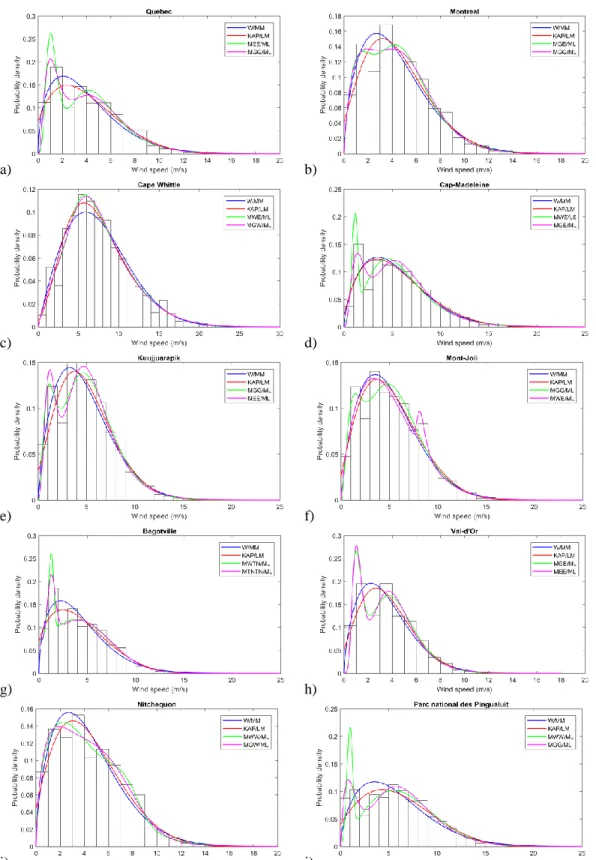
In Fig. 4, the histograms of the observed wind speed data at the 10 stations selected to
439
illustrate the results for the prince of Quebec are presented. W and KAP as well as the first and
440
second mixture distribution models providing the best fit to the data according to 2 are
441
superimposed in these histograms. Table 4 lists the four best models at each station according to
442
each criterion. Mixture distributions have in general higher ranks than one-component
443
distributions. The flexibility and advantages of mixture distribution models are illustrated in Fig.
444
4 as one-component distributions are shown not to be suitable to model all stations. For instance,
445
mixture distributions are necessary to model stations Quebec, Cap-Madeleine, Bagotville,
Val-446
d’Or and Parc national des Pingualuit. Even for stations presenting unimodal behaviors, such as
447
the stations of Montréal, Cape Whittle, Mont-Joli, Kuujjuarapik and Nitchequon, mixture
448
distributions provide also, in general, the best goodness-of-fit statistics according to the ranks in
449
Table 4.
450
24 6. Conclusions and future work
452
In this study, we evaluate the suitability of a selection of homogeneous and
453
heterogeneous two-component distributions as well as a number of one-component distributions
454
including W and KAP to model wind speed data in a Nordic environment. The case study is
455
represented by 83 meteorological stations distributed throughout the wide territory of the
456
province of Québec, Canada. The approach consisted first in using the L-moment ratio diagrams
457
to assess the one-component distributions that best fit the data. Among the pdfs defining a curve
458
(probability distributions having one shape parameter) on the MRD, W is the pdf leading to the
459
best fit. For the distributions with two shape parameters, GG, LP3 and KAP, areas of feasibility
460
are defined in the MRD diagram and these distributions can represent better alternatives for the
461
stations whose data samples are located the farthest from the curve defined by W.
462
MRDs are not able to represent distributions presenting bimodal behaviors. Mixture
463
distributions can be used to model such behavior. A selection of 10 two-component distributions
464
mixing W, G, E and TN were fitted to the wind speed at the stations of the study area. The
465
parameters were estimated with the LS and ML methods. Results were compared to the fit
466
obtained by the most adequate one-component distributions: the W and KAP distributions.
467
Global results indicated that mixture models provide better goodness-of-fit than the W and KAP
468
according to the performance criteria used. It was found that the ML method outperforms the LS
469
method according to all criteria. Mixture distributions are flexible and can efficiently model both
470
bimodal and unimodal behaviors.
471
The results of the present study show that mixture distribution models have the potential
472
to improve the estimation of energy generation potential at stations presenting bimodal regimes
25
and even at stations presenting unimodal regimes. Improved accuracy in wind energy potential
474
assessment can help with site selection and with the design and management of wind farms. The
475
proposed methods are general and can be transposed to other regions especially those where
476
pronounced bimodal regimes are observed.
477
10 stations with a good distribution across the study area were selected to illustrate the
478
results of the study. The histograms of the fitting of the one-component and mixture models to
479
the wind speed data at the 10 selected stations are presented. The analysis of the histograms of
480
the wind speed data at each station have shown that a bimodal behavior was observed in about 5
481
stations. For these stations, mixture distributions reveal to be necessary in order to adequately
482
model the wind speed distributions.
483
It is important to note that the mixture models applied in this study present additional
484
complexity in comparison to simpler models such the one-component Weibull. Parameter
485
estimation for mixture models requires advanced optimization method such as the genetic
486
algorithm used here. This method takes more time to process than other optimization methods.
487
This can be cumbersome when the mixture approach is applied to a large number of stations for
488
instance.
489
The MRD approach needs to be extended to bimodal and mixture distributions in order to
490
be useful for the whole range of distributions of interest for wind energy assessment and
491
modeling. Future work should also focus on the analysis of the non-stationarity in wind speed
492
data (presence of trends, jumps and cycles) in the province of Quebec in order to provide reliable
493
estimates of the future potential for wind energy generation. The frequency analysis models used
494
in the present study and in most literature dealing with wind speed modeling are based on the
26
hypothesis of the stationarity of the wind speed regime. Unfortunately, such assumption is often
496
invalid, and past wind speed observations are not necessarily representative of the future wind
497
speed regime. Increasing attention is being devoted to the development of non-stationary
498
frequency modeling tools for climatic variables, which take into consideration information about
499
climate change (see for instance Lee and Ouarda, 2011; Chandran et al., 2016).
500
Future work should also focus on the extension of homogeneous and heterogeneous
501
mixture models to the non-stationary case. The resulting models will have distribution
502
parameters that are dependent on the values of covariates that may represent time or climate
503
indices. A non-stationary frequency analysis of wind speed data in the province of Quebec can
504
also integrate low frequency climate oscillation indices as covariates to take into consideration
505
information concerning the impact of these climatic indices on the inter-annual variability in
506
wind speed in the region. Such models are becoming increasingly popular in climatology and
507
renewable energy modeling (see for instance Ouachani et al., 2013; Naizghi and Ouarda, 2017)
508
and would allow understanding the teleconnections of wind characteristics with various global
509
climate indices and examining the long-term variability of wind speed in the province.
510
Thiombiano et al. (2017) have already identified the Arctic Oscillation (AO) and the Pacific
511
North American (PNA) climate indices as the dominant indices in the region. These indices can
512
be integrated relatively easily in the models developed in the present work.
513
514
515
Acknowledgements 516
27
Financial support for the present study was provided by the Natural Sciences and Engineering 517
Research Council of Canada (NSERC). The authors wish to thank Environment and Climate Change
518
Canada for having supplied the wind speed data used in this study. The authors are grateful to the
519
Editor-in-Chief, Dr. Marc Rosen, and to two anonymous reviewers for their comments which
520
helped improve the quality of the manuscript.
521
28 References
523
Acker, T.L., Williams, S.K., Duque, E.P.N., Brummels, G., Buechler, J., 2007. Wind resource assessment 524
in the state of Arizona: Inventory, capacity factor, and cost. Renewable Energy, 32(9): 1453-1466. 525
doi:10.1016/j.renene.2006.06.002. 526
Ahmed Shata, A.S., Hanitsch, R., 2006. Evaluation of wind energy potential and electricity generation on 527
the coast of Mediterranean Sea in Egypt. Renewable Energy, 31(8): 1183-1202. doi: 528
10.1016/j.renene.2005.06.015. 529
Akpinar, E.K., Akpinar, S., 2005. An assessment on seasonal analysis of wind energy characteristics and 530
wind turbine characteristics. Energy Conversion and Management, 46(11-12): 1848-1867. 531
doi:10.1016/j.enconman.2004.08.012. 532
Akpinar, S., Akpinar, E.K., 2009. Estimation of wind energy potential using finite mixture distribution 533
models. Energy Conversion and Management, 50(4): 877-884. doi:10.1016/j.enconman.2009.01.007. 534
Archer, C.L., Jacobson, M.Z., 2003. Spatial and temporal distributions of U.S. winds and wind power at 535
80 m derived from measurements. Journal of Geophysical Research: Atmospheres, 108(D9): 4289. 536
doi:10.1029/2002jd002076. 537
Ayodele, T.R., Jimoh, A.A., Munda, J.L., Agee, J.T., 2012. Wind distribution and capacity factor 538
estimation for wind turbines in the coastal region of South Africa. Energy Conversion and 539
Management, 64: 614-625. doi:10.1016/j.enconman.2012.06.007. 540
Barbet, M., Bruneau, P., Ouarda, T.B.M.J., Gingras, H., 2006. REGIONS – Software for regional flood 541
estimation. HYDRO-2006 conference: Maximizing the benefits of hydropower, Porto-Carras, 542
Greece, 25th -28th September 2006. 543
29
Carrasco-Díaz, M., Rivas, D., Orozco-Contreras, M., Sánchez-Montante, O., 2015. An assessment of 544
wind power potential along the coast of Tamaulipas, northeastern Mexico. Renewable Energy, 78: 545
295-305. doi:10.1016/j.renene.2015.01.007. 546
Carta, J.A., Ramírez, P., 2007. Use of finite mixture distribution models in the analysis of wind energy in 547
the Canarian Archipelago. Energy Conversion and Management, 48(1): 281-291. 548
doi:10.1016/j.enconman.2006.04.004. 549
Carta, J.A., Ramirez, P., Velazquez, S., 2008. Influence of the level of fit of a density probability function 550
to wind-speed data on the WECS mean power output estimation. Energy Conversion and 551
Management, 49(10): 2647-2655. doi:10.1016/j.enconman.2008.04.012. 552
Carta, J.A., Ramirez, P., Velazquez, S., 2009. A review of wind speed probability distributions used in 553
wind energy analysis Case studies in the Canary Islands. Renewable & Sustainable Energy Reviews, 554
13(5): 933-955. doi:10.1016/j.rser.2008.05.005. 555
Carter, W.H., Bowen, J.V., Myers, R.H., 1971. Maximum likelihood estimation from grouped Poisson 556
data. Journal of the American Statistical Association, 66(334): 351-353. 557
doi:10.1080/01621459.1971.10482267. 558
Celik, A.N., 2003. Energy output estimation for small-scale wind power generators using Weibull-559
representative wind data. Journal of Wind Engineering and Industrial Aerodynamics, 91(5): 693-707. 560
doi:10.1016/s0167-6105(02)00471-3. 561
Chandran, A., Basha, G., Ouarda, T.B.M.J., 2016. Influence of climate oscillations on temperature and 562
precipitation over the United Arab Emirates. International Journal of Climatology, 36(1): 225-235. 563
doi:10.1002/joc.4339. 564
Chang, T.P., 2011. Estimation of wind energy potential using different probability density functions. 565
Applied Energy, 88(5): 1848-1856. doi:10.1016/j.apenergy.2010.11.010. 566
30
Dabbaghiyan, A., Fazelpour, F., Abnavi, M.D., Rosen, M.A., 2016. Evaluation of wind energy potential 567
in province of Bushehr, Iran. Renewable and Sustainable Energy Reviews, 55: 455-466. 568
doi:10.1016/j.rser.2015.10.148. 569
El Adlouni, S., Bobée, B., Ouarda, T.B.M.J., 2008. On the tails of extreme event distributions in 570
hydrology. Journal of Hydrology, 355(1-4): 16-33. doi:10.1016/j.jhydrol.2008.02.011. 571
El Adlouni, S., Ouarda, T.B.M.J., 2007. Orthogonal projection L-moment estimators for three-parameter 572
distributions. Advances and Applications in Statistics, 7(2): 193-209. 573
Greenwood, J.A., Landwehr, J.M., Matalas, N.C., Wallis, J.R., 1979. Probability weighted moments: 574
Definition and relation to parameters of several distributions expressable in inverse form. Water 575
Resources Research, 15(5): 1049-1054. doi:10.1029/WR015i005p01049. 576
Gouvernement du Québec, 2016. Politique énergétique 2030. Retrieved from: 577
http://politiqueenergetique.gouv.qc.ca/wp-content/uploads/politique-energetique-2030.pdf
578
Hassanzadeh, Y., Abdi, A., Talatahari, S., Singh, V.P., 2011. Meta-Heuristic Algorithms for Hydrologic 579
Frequency Analysis. Water Resources Management, 25(7): 1855-1879. doi:10.1007/s11269-011-580
9778-1. 581
HE&AWS, 2005. Inventaire du potentiel éolien exploitable du Québec, Hélimax Énergie inc., AWS 582
Truewind, LLC. Retrieved from:
583
http://www.mrn.gouv.qc.ca/publications/energie/eolien/vent_inventaire_inventaire_2005.pdf
584
Hosking, J.R.M., 1990. L-Moments: Analysis and estimation of distributions using linear combinations of 585
order statistics. Journal of the Royal Statistical Society, Series B (Methodological), 52(1): 105-124. 586
doi:10.2307/2345653. 587
31
Hosking, J.R.M., 1994. The four-parameter kappa distribution. IBM Journal of Research and 588
Development, 38(3): 251-258. doi:10.1147/rd.383.0251. 589
Hosking, J.R.M., 1996. Fortran routines for use with the method of L-moments, version 3.04. 20525, IBM 590
Research Division, Yorktown Heights, N.Y. 591
Hosking, J.R.M., Wallis, J.R., 1997. Regional frequency analysis: An approach based on L-Moments. 592
Cambridge University Press, New York, 240 pp. 593
Hundecha, Y., St-Hilaire, A., Ouarda, T.B.M.J., El Adlouni, S., Gachon, P., 2008. A Nonstationary 594
Extreme Value Analysis for the Assessment of Changes in Extreme Annual Wind Speed over the 595
Gulf of St. Lawrence, Canada. Journal of Applied Meteorology and Climatology, 47(11): 2745-2759. 596
doi:10.1175/2008jamc1665.1. 597
Ilinca, A., McCarthy, E., Chaumel, J.-L., Rétiveau, J.-L., 2003. Wind potential assessment of Quebec 598
Province. Renewable Energy, 28(12): 1881-1897. doi:10.1016/S0960-1481(03)00072-7. 599
Irwanto, M., Gomesh, N., Mamat, M.R., Yusoff, Y.M., 2014. Assessment of wind power generation 600
potential in Perlis, Malaysia. Renewable and Sustainable Energy Reviews, 38: 296-308. 601
doi:10.1016/j.rser.2014.05.075. 602
Jaramillo, O.A., Borja, M.A., 2004. Wind speed analysis in La Ventosa, Mexico: a bimodal probability 603
distribution case. Renew. Energy, 29(10): 1613-1630. doi:10.1016/j.renene.2004.02.001. 604
Jung, C., Schindler, D., 2017. Global comparison of the goodness-of-fit of wind speed distributions. 605
Energy Conversion and Management, 133: 216-234. doi:10.1016/j.enconman.2016.12.006. 606
Jung, C., Schindler, D., Laible, J., Buchholz, A., 2017. Introducing a system of wind speed distributions 607
for modeling properties of wind speed regimes around the world. Energy Conversion and 608
Management, 144: 181-192. doi:10.1016/j.enconman.2017.04.044. 609
32
Kollu, R., Rayapudi, S.R., Narasimham, S., Pakkurthi, K.M., 2012. Mixture probability distribution 610
functions to model wind speed distributions. International Journal of Energy and Environmental 611
Engineering, 3(1): 1-10. doi:10.1186/2251-6832-3-27. 612
Lee, T., Ouarda, T.B.M.J., 2011. Prediction of climate nonstationary oscillation processes with empirical 613
mode decomposition. Journal of Geophysical Research: Atmospheres, 116: D06107. 614
doi:10.1029/2010jd015142. 615
Lo Brano, V., Orioli, A., Ciulla, G., Culotta, S., 2011. Quality of wind speed fitting distributions for the 616
urban area of Palermo, Italy. Renewable Energy, 36(3): 1026-1039. 617
doi:10.1016/j.renene.2010.09.009. 618
Masseran, N., Razali, A.M., Ibrahim, K., 2012. An analysis of wind power density derived from several 619
wind speed density functions: The regional assessment on wind power in Malaysia. Renewable & 620
Sustainable Energy Reviews, 16(8): 6476-6487. doi:10.1016/j.rser.2012.03.073. 621
Mazzeo, D., Oliveti, G., Labonia, E., 2018. Estimation of wind speed probability density function using a 622
mixture of two truncated normal distributions. Renewable Energy, 115: 1260-1280. 623
doi:10.1016/j.renene.2017.09.043. 624
Morgan, E.C., Lackner, M., Vogel, R.M., Baise, L.G., 2011. Probability distributions for offshore wind 625
speeds. Energy Conversion and Management, 52(1): 15-26. doi:10.1016/j.enconman.2010.06.015. 626
Naizghi, M.S., Ouarda, T.B.M.J., 2017. Teleconnections and analysis of long-term wind speed variability 627
in the UAE. International Journal of Climatology, 37(1): 230-248. doi:10.1002/joc.4700. 628
Ouachani, R., Bargaoui, Z., Ouarda, T.B.M.J., 2013. Power of teleconnection patterns on precipitation 629
and streamflow variability of upper Medjerda Basin. International Journal of Climatology, 33(1): 58-630
76. doi:10.1002/joc.3407. 631
33
Ouarda, T.B.M.J., Ashkar, F., 1998. Effect of Trimming on LP III Flood Quantile Estimates. Journal of 632
Hydrologic Engineering, 3(1): 33-42. doi:10.1061/(ASCE)1084-0699(1998)3:1(33). 633
Ouarda, T.B.M.J.,Charron, C., 2018. Distributions of wind speed in a northern environment, 2018 9th 634
International Renewable Energy Congress (IREC), Hammamet, Tunisia, pp. 1-3. 635
DOI:10.1109/IREC.2018.8362453 636
Ouarda, T.B.M.J., Charron, C., Chebana, F., 2016. Review of criteria for the selection of probability 637
distributions for wind speed data and introduction of the moment and L-moment ratio diagram 638
methods, with a case study. Energy Conversion and Management, 124: 247-265. 639
doi:10.1016/j.enconman.2016.07.012. 640
Ouarda, T.B.M.J., Charron, C., Shin, J.Y., Marpu, P.R., Al-Mandoos, A.H., Al-Tamimi, M.H., Ghedira, 641
H., Al Hosary, T.N., 2015. Probability distributions of wind speed in the UAE. Energy Conversion 642
and Management, 93: 414-434. doi:10.1016/j.enconman.2015.01.036. 643
Petković, D., Shamshirband, S., Anuar, N.B., Saboohi, H., Abdul Wahab, A.W., Protić, M., Zalnezhad, 644
E., Mirhashemi, S.M.A., 2014. An appraisal of wind speed distribution prediction by soft computing 645
methodologies: A comparative study. Energy Conversion and Management, 84: 133-139. 646
doi:10.1016/j.enconman.2014.04.010. 647
Seckin, N., Haktanir, T., Yurtal, R., 2011. Flood frequency analysis of Turkey using L‐moments method. 648
Hydrological Processes, 25(22): 3499-3505. doi:10.1002/hyp.8077. 649
Shin, J.-Y., Ouarda, T.B.M.J., Lee, T., 2016. Heterogeneous mixture distributions for modeling wind 650
speed, application to the UAE. Renewable Energy, 91: 40-52. doi:10.1016/j.renene.2016.01.041. 651
Soukissian, T., 2013. Use of multi-parameter distributions for offshore wind speed modeling: The 652
Johnson SB distribution. Applied Energy, 111: 982-1000. doi:10.1016/j.apenergy.2013.06.050. 653
34
Soukissian, T.H., Karathanasi, F.E., 2017. On the selection of bivariate parametric models for wind data. 654
Applied Energy, 188: 280-304. doi:10.1016/j.apenergy.2016.11.097. 655
Thiombiano, A.N., El Adlouni, S., St-Hilaire, A., Ouarda, T.B.M.J., El-Jabi, N., 2017. Nonstationary 656
frequency analysis of extreme daily precipitation amounts in Southeastern Canada using a peaks-657
over-threshold approach. Theoretical and Applied Climatology, 129(1): 413-426. 658
doi:10.1007/s00704-016-1789-7. 659
Tuller, S.E., Brett, A.C., 1983. The characteristics of wind velocity that favor the fitting of a Weibull 660
distribution in wind speed analysis. Journal of Climate and Applied Meteorology, 23. 661
Yip, C.M.A., Gunturu, U.B., Stenchikov, G.L., 2016. Wind resource characterization in the Arabian 662
Peninsula. Applied Energy, 164: 826-836. doi:10.1016/j.apenergy.2015.11.074. 663
Zhou, J.Y., Erdem, E., Li, G., Shi, J., 2010. Comprehensive evaluation of wind speed distribution models: 664
A case study for North Dakota sites. Energy Conversion and Management, 51(7): 1449-1458. 665
doi:10.1016/j.enconman.2010.01.020. 666
667
35
Table 1. List of probability density functions, domains, and list of parameters.
Name Probability density function Domain Number of
parameters E E 1 ( ; , ) exp x exp x f x x 2 W 1 W( ; , ) exp k k k x x f xk 0 x 2 G G( ; , ) 1exp( ) k k f x k x x k 0 x 2 LN 2 LN 2 ln 1 ( ; , ) exp 2 2 x f x x 0 x 2 GG 1 GG( ; , , ) exp( ) hk hk h h f x k h x x k 0 x 3 P3 P3( ; , , ) 1exp k k f x k x x k x 3 GEV 1 1 1/ LN 1 ( ; , , ) 1 exp 1 k k k k f x k x u x u / if 0 / if 0 if 0 u k x k x u k k x k 3 LP3 1
LP3( ; , , ) log exp log
k a a g f x k x x x k where glogae /g /g if 0 0 if 0 e x x e 3 KAP 1 1/ 1 1 KAP( , , , ) [1 ( ) / ] [ KAP( )] k h f k h k x F x where 1/ 1/ KAP( ) (1 (1 ( ) / ) ) k h F x h k x if 0, 0 (1 ) / / if 0, 0 (1 ) / / if 0, 0 / if 0, 0 k k h k h k x k h k h k x x k h k k x h k 4 μ: location parameter α: scale parameter k: shape parameter
h: second shape parameter (GG, KAP) Γ( ): gamma function
36 Table 2. List of mixture probability density functions, domains.
Name Probability density function Domain
MGG fGG( ;x1,k1,2,k2)fG( ;x1,k1) (1 )fG( ;x2,k2) 0 x MGW fGW( ;x1,k1,2,k2)fG( ;x1,k1) (1 )fW( ;x2,k2) 0 x MGE fGE( ;x1, , ,k 2)fG( ;x1, )k (1 )fE( ; ,x 2) x MGTN fGN( ;x1, , ,k 2)fG( ;x1, )k (1 )fTN( ; ,x 2) 0 x MWW fWW( ;x1,k1,2,k2)fW( ;x1,k1) (1 )fW( ;x2,k2) 0 x MWE fWE( ;x1, , ,k 2)fW( ;x1, )k (1 )fE( ; ,x 2) x MEE fEE( ;x 1, 1, 2, 2)fE( ;x 1, 1) (1 )fE( ;x 2, 2) x METN fEN( ;x 1, 1, 2, 2)fE( ;x 1, 1) (1 )fTN( ;x 2, 2) x MTNTN fNN( ;x 1, 1, 2, 2)fTN( ;x 1, 1) (1 )fTN( ;x 2, 2) 0 x