Stream Temperature Modeling Using Functional Regression Models.

Technical Paper

Running Author: Boudreault, Bergeron, St‐Hilaire, and Chebana

Running Title: Stream Temperature Modeling Using Functional Regression Models

Stream Temperature Modeling Using Functional

Regression Models

Water, Earth and Environment Center, National Institute of Scientific Research (INRS‐ ETE), Québec City, Québec, CAN

Water, Earth and Environment Center, National Institute of Scientific Research (INRS‐ETE), Québec City, Québec, CAN (Correspondence to St‐Hilaire: [email protected]).

Abstract

Stream temperature is one of the most important environmental variables in lotic habitats as it has important and direct impacts on the ecosystem. Given the continuous nature of this variable, the aim of this paper was to introduce functional regression for the air‐stream temperature relation, being capable to model an entire seasonal or annual curve of temperatures as one entity, rather than multiple daily or weekly values in classical models. Three types of functional models were explored in the study and compared to two classical models (Generalized Additive Model and Logistic Model) for six rivers from the United States The results show the functional models have the best performance for all the considered rivers. When comparing functional models between them, one variant of the historical functional model performs better than the two other models and is the most parsimonious. Functional regression leads to encouraging results to model the complete annual stream temperature curve as one entity compared to other classical approaches.

Received: 26 July 2018 | Accepted: 16 May 2019

Keywords

environmental indicators; temperature; stream temperature; statistics; functional regression; modeling;

Paper No. JAWRA‐18‐0108‐P of the Journal of the American Water Resources Association (JAWRA).

1 1 1 1

Research Impact Statement: By modeling the stream temperature curve rather than scalar daily values, functional regression models better represent the stream temperature variable and perform better than other classical models.

Data Availability Statement: All data used in this study are freely available and can be downloaded directly from the NOAA (for air temperatures) and USGS (for stream temperatures) websites (links available in the following references).

INTRODUCTION

Stream temperature is one of the most important characteristics when studying aquatic ecosystems (Beschta et al. 1987; Caissie 2006). Many fishes are sensitive to water temperature, especially during growth and spawning periods (Handeland et al. 2008). Their ability to correctly perform their biological functions can be severely affected if the water temperature is inadequate (Lee and Rinne 1980; Sigholt and Finstad 1990; Bjornn and Reiser 1991). Furthermore, the thermal regime of a river can be modified through human activities. For instance, deforestation influences the canopy cover, which causes changes to the heat input into the river (Beschta et al. 1987). In addition, Webb and Walling (1993) showed that flow regulation can increase mean value of the stream temperatures. More recently, Maheu et al. (2016) found that the presence of dams on medium size rivers in Eastern Canada causes an increase in their September monthly mean temperature. Finally, global warming is typically expected to cause increases in stream temperature that are likely to continue in the future with a higher amplitude (Morrison et al. 2002; Kaushal et al. 2010; Isaak et al. 2012), which will affect thermal‐sensitive fish species such as salmonids (e.g., Rieman et al. 2007; Isaak et al. 2010; Hedger et al. 2013; Holsinger et al. 2014; Isaak, Luce, et al. 2018).

Models that predict and simulate stream temperature are therefore needed. They can be divided in two main categories: deterministic and statistical models (Benyahya, Caissie, et al. 2007). The former focus on mathematical relations that characterize the physical processes of heat transfer and link the stream temperature to other hydro‐meteorological and physical variables, based on an energy budget approach (Morin et al. 1981). However, these models require several input variables and are often costly in computation time (Benyahya, Caissie, et al. 2007). Indeed, most mechanistic thermal models require multiple, spatially distributed meteorological inputs such as solar radiation (both short and long wave), wind velocity, vapor pressure, cloud cover, etc. In addition, discharge and/or water levels are often required as a prelude to the heat budget calculation to be performed on a known water volume. Statistical models typically use fewer predictors, less computational time and often lead to more simplicity than deterministic models. Statistical models in stream temperature include nonparametric approaches like the artificial neural network (Bélanger et al. 2005; Chenard and Caissie 2008; DeWeber and Wagner 2014; Piotrowski et al. 2015) and the k‐nearest neighbors (KNN) model (Benyahya et al. 2008; St‐ Hilaire et al. 2012). On the other hand, parametric models can be stochastic or regression‐ based. Times series models are among the former and include second‐order Markov process (Cluis 1972; Caissie et al. 1998; Caissie et al. 2001), periodic autoregressive model (Benyahya, St‐Hilaire et al. 2007) and nonlinear autoregressive process with exogenous variable (Kwak et al. 2017). In the regression models, the stream temperature is modeled as a function of one or multiple predictors. This relation is often assumed to be linear (Crisp and Howson 1982; Jeppesen and Iversen 1987; Mackey and Berrie 1991; Jourdonnais et al. 1992; Stefan and Preud'homme 1993) or nonlinear like the logistic model (LM) of Mohseni et al. (1998), the Gaussian process of Grbić et al. (2013) and the generalized additive model (GAM) (Wehrly et al. 2009; Laanaya et al. 2017). However, regression models can suffer from collinearity when significant correlation exists between predictors and thus, a Ridge regression can be used to overcome this problem (Ahmadi‐Nedushan et al. 2007).

For all the aforementioned models and others described in the literature, stream temperature data are considered in a punctual or discrete manner, as it is recorded. However, stream temperature is naturally a continuous variable and shows a strong seasonal pattern. Hence, it can be better represented by a curve over a year or a season rather than using aggregate values such as a mean over a certain period or with multiple correlated observations. For some current methods, a serious loss of information is made when aggregating many values, which is not the case when working with an entire curve of stream temperatures. For example, the LM of Mohseni et al. (1998) performs better with weekly mean temperatures than daily, given the greater autocorrelation in daily data (Pilgrim et al. 1998; Morrill et al. 2005; Caissie 2006; Benyahya, Caissie, et al. 2007). For the above reasons, it is of interest to introduce Functional Data Analysis (FDA) in this context. FDA is a framework that uses curves or functions as observations, in contrast with scalar or vectors in other classical frameworks in statistics. Hence, working with a curve instead of daily, weekly, or monthly metrics naturally leads to a better description and understanding of the whole phenomenon and captures more of its variability (Chebana et al. 2012). Another interesting fact about using FDA in this context is to avoid collinearity in the predictors used in regression models. For example, models using air temperature at different time scales, for example, at t − 1 and t − 2, to model stream temperature at t, will suffer from possible redundancy as the air temperature series is highly autocorrelated. However, with FDA, this problem is avoided as the whole curve of predictor values (in this study, air temperature) can be used as a single input (Cuevas et al. 2002). This also means that FDA inherently handles seasonality in the data, whereas other regression models will need either a prior step to remove it or the addition of an extra covariate to take it in account (Caissie 2006; Laanaya et al. 2017). Finally, in the functional framework, the prediction error remains constant over the modeled period because it is a single simulated curve, whereas this error can increase when using time series approaches (Box et al. 2015). On the other hand, as FDA uses curves instead of scalars or vectors, a year of daily records will only be n = 1 functional observation in FDA, whereas it corresponds to n = 365 observations in the classical models, which means that many years of records will be needed to adequately calibrate a functional regression model (Ramsay 2006). Finally, FDA requires that the studied phenomena are smooth enough, which does not create any problem for air and stream temperature series, but may be problematic for other meteorological variables such as rainfall that is characterized by greater stochasticity than temperature (Suhaila et al. 2011; Masselot et al. 2016).

FDA was introduced by Ramsay (1982) and became very popular and present in the literature during the last decade, with multiple textbooks (Ferraty and Vieu 2006; Ramsay 2006; Dabo‐ Niang and Ferraty 2008; Ramsay et al. 2009; Bosq 2012) and recent applications in various fields including ecology, transportation (Chiou 2012), energy (Chaouch 2014; Brockhaus et al. 2015), waste management (Bernardi et al. 2017), biotechnology (Brockhaus, Melcher, et al. 2017), medicine (Ciarleglio et al. 2016), neuroscience (McLean et al. 2014; Ivanescu et al. 2015; Meyer et al. 2015). Chebana et al. (2012) were the first to introduce FDA in the hydrological context, seeing the annual series of streamflow, the hydrograph, as a curve, that is, a functional datum. Many recent studies have applied FDA to the streamflow variable (i.e., Masselot et al. 2016; Ternynck et al. 2016; Brunner et al. 2017; Larabi et al. 2017; Requena et al. 2018), whereas no attempt has been made to model the stream temperature curve. Similarly to streamflow, where the hydrograph was seen as a curve over a year (Chebana et al. 2012), stream temperature can also be adequately represented using a single annual curve, especially given its pronounced seasonal trend. Hence, the aim of this work is to introduce the FDA framework to the stream temperature modeling with a focus on functional regression models.

Segura et al. 2015) and the GAM (Wehrly et al. 2009; Laanaya et al. 2017). As a generalization of the LM, GAM allows for more flexibility and was recently shown in one case study to be the best model for daily mean stream temperature compared to other models (Laanaya et al. 2017).

METHODS

Functional Regression Models

FDA aims at working with functions (curves) instead of discrete observations. Because data are not recorded continuously, a first step in FDA is to convert discrete recorded observations to functions by smoothing techniques. This can be achieved by defining a function x(t) as a weighted sum of M known basis functions that adequately represent the given discrete observations (Ramsay 2006):

(1)

where c and ϕ (t) are, respectively, the coefficients to be estimated and the basis functions. For periodic data, a Fourier series expansion is often used as basis functions, and for nonperiodic data the most popular basis functions are B‐splines (Ramsay 2006). Once the data curves have been constructed, the functional data (i.e., the curves) are ready to be used in the FDA framework including functional regression models.

In the standard linear regression model, values of all variables are scalar (Neter et al. 1996). In the functional case, three possible scenarios occur (Morris 2015). The scalar‐on‐function models, where at least one of the predictors is functional but the predictand is a scalar. Conversely, in the function‐on‐scalar models, the predictand is functional but all the predictors are scalar values. The last one is the function‐on‐function models, where the predictand and at least one of the predictors are functional (Ramsay 2006).

As a first attempt to model the stream temperature curve, only one predictor will be used: the air temperature curve. Even if air temperature is not the major driver of water temperature increase or decrease (Sullivan and Adams 1991; Johnson 2003), it is, however, a good substitute in statistical models of complex heat flux equations (Webb 1987) and has been used in many other studies to model stream temperature with success (Caissie 2006; Benyahya, Caissie, et al. 2007). Hence, to model the stream temperature curve from the air temperature curve, it is appropriate to consider the function‐on‐function models. First, the simplest model in this class is called the concurrent model (Ramsay 2006). It is the analogue to the linear model with functional observations:

(2)

where y (.) and x (.) represent, respectively, the curves of stream and air temperatures for the year i and day t and the domain Ω is the same for both y(t) and x(t). Note that in this model, the intercept α(t) and the regression coefficient β(t) are also functions. Basically, their expressions are of the same nature as of y(t) and x(t) (Equation 1), that is, linear combination of basis

x (t) =

∑

(t) , t ∈

,

c

ϕ

Ω

(t) = α (t) + β (t) (t) + (t) , t ∈

,

y

x

ε

Ω

functions. Model (2) only allows the predictor x (.) to influence y (.) at the same time t or at a fixed lag t − l. However, the predictand at time t can be affected by the predictor at different times. In the case of stream temperature, it can take several days before a rise or fall in air temperature induces a change in stream temperature. Hence, the concurrent model in (Equation 2) is not suitable to incorporate this heat exchange process and the fully functional linear model (FFLM) should be introduced:

(3)

where β(s,t) is a surface representing the effect of x (.) at time s on y (.) at any time t. The domain Ω of s can differ from the domain Ω of t. In this model, all the values of x (.) are used to model the value of y (.) at any time t. In Masselot et al. (2016), FFLM (Equation 3) was used to model streamflow curve from the precipitation curve, allowing lagged effect of the precipitation on the streamflow, that is, precipitations occurring at s > t were used to model streamflow at t. Even if from a meteorological point of view precipitations occurring at s  >  t cannot affect the streamflow at time t, the β(s,t) surface was close to 0 for s > t, motivating the use of the FFLM with those variables. In the case considered here, it is more appropriate to introduce the historical functional linear model (HFLM) as it allows to restrict the domain where the predictor influences the predictand (Malfait and Ramsay 2003; Harezlak et al. 2007; Gervini 2015). The HFLM has known recent developments regarding its implementation (Brockhaus et al. 2015; Brockhaus, Melcher, et al. 2017) and is defined as follows:

(4)

where l(t) and u(t) are, respectively, the lower and the upper bound where the predictor x (.) can influence y (.) at time t. This model allows an important flexibility with particular cases of interest. For instance, if all past values of x (.) affect y (.) at t, then l(t) = 0 and u(t) = t. If only the past values of a series of length d affect x (.) on y (.) at t, then l(t) = max(0, t − d) and u(t) = t (Malfait and Ramsay 2003; Kim et al. 2011). For comparison, three functional regression models will be used in this study:

1. FFLM (Equation 3)

2. HFLM1 (Equation 4), with l(t) = 0 and u(t) = t

3. HFLM2 (Equation 4), with l(t) = max(0, t − d), u(t) = t, and d = 15

The choice of d  =  15 was motivated by the fact that there is a lag between a change in air temperature and the resulting change in the stream temperature series especially for larger systems. Hence, a period of 15 days should typically be enough to include and represent this lag (Preud'homme and Stefan 1992).

i i

(t) = α (t) +

β (s, t) (s) ds + (t) , t ∈

,

y

∫

x

ε

Ω

(t) = α (t) +

β(t, s) (s)ds + (t) , t ∈

,

y

∫

x

ε

Ω

In order to fit functional models, the functional linear array model (FLAM) implemented in R (R Core Team 2017) by Brockhaus et al. (2015) in the package FDboost (Brockhaus, Ruegamer, et al. 2017) was used as it can fit both model (3) and (4) with different configurations of l(t) and u(t). The FLAM is fitted using a component‐wise gradient boosting algorithm, a machine learning procedure that estimates the model parameters by minimizing an empirical loss function (Freund et al. 1999; Bühlmann and Hothorn 2007; Brockhaus, Melcher, et al. 2017). In our case, the minimized loss function is the root mean squared error (Brockhaus et al. 2015):

(5)

where is the simulated stream temperature curve by the functional model. The minimization procedure is iterative and each iteration leads to a rougher β(s,t) surface (Brockhaus et al. 2015). The minimization procedure is halted when the mean square error calculated with a leave‐one‐out validation procedure is minimized, leading to more regularized effects (i.e., smoother β(s,t) surface) and more stable predictions (Brockhaus, Rügamer, et al. 2017). More information about the FLAM, the FDboost package and the boosting algorithm can be found in the above references.

Generalized Additive Model

This model was introduced by Hastie and Tibshirani (1990) as an extension of the generalized linear model, without the assumption of linearity in the relationship between predictors and the predictand, as well as relaxing the normality assumption. Even if only few applications of the GAM in stream temperature have been reported (Wehrly et al. 2009; Laanaya et al. 2017), it has been widely used in hydrology (Chebana et al. 2014; Zhang et al. 2015; Falah et al. 2017; Iddrisu et al. 2017; Rahman et al. 2018). GAM is defined as follows:

(6)

where g is the link function, E(y) is the expected value of the predictand (in our case, the daily mean stream temperature), x is the jth predictor, f is the associated smooth nonlinear function (often combination of cubic splines), and ε is the error term. Here, we use the identity function as link function g(.) and two covariates, x the Julian day of year to account for the seasonality in stream temperature data and x the daily mean air temperature as previously done in Laanaya et al. (2017). The inclusion of an additional predictor that accounts for seasonality in the GAM, f (x ), where x is the Julian day of year, will make the comparability between GAM and functional models more reliable, as functional models inherently handle seasonality, whereas GAM require the inclusion of an extra covariate to do so (Laanaya et al. 2017).

To avoid overfitting, a penalized GAM is used and fitted by minimizing an error term calculated by cross‐validation with the package mgcv (minimized generalized cross‐validation) (Wood 2006; Wood 2015) in R (R Core Team 2017).

dt,

1

n

∑

[ (t) −

(t)]

∫

y

y^

−

−−−−−−−−−−−−−−−−−−−−

−



⎷





(. )

y^

g(E(y) =

f

( ) +

x

f

( ) + … +

x

f

( ) + ε,

x

Logistic Model

As highlighted in Mohseni et al. (1998), the relation between air and stream temperatures can be represented with a continuous S‐shaped function better than with a linear regression. A common function to model this relation is the logistic function (denoted LM) defined as follows:

(7)

where T and T are, respectively, stream and air mean temperatures. The parameters to be adjusted are α: the estimated maximum stream temperature, γ: the measure of the steepest slope and β: the air temperature inflection point. Mohseni et al. (1998) first used the logistic function to estimate the whole year of weekly stream temperatures data for different watercourses in the United States (U.S.). In our case and for comparison purposes, the LM model is applied on daily summer mean temperature as done in recent applications (Kelleher et al. 2012; St‐Hilaire et al. 2012; Grbić et al. 2013; Bustillo et al. 2014; Laanaya et al. 2017).

Performance Criteria

To assess model performances, criteria commonly used in the context of stream temperature are calculated for each model as well as new functional criteria. A cross‐validation technique called the annual leave‐one‐out cross‐validation method is used (Quenouille 1949). Basically, one year of observed data is temporarily removed prior to fitting each model. Then, the fitted model is used to simulate the stream temperature for the year that was removed. The performance criteria are then calculated based on the simulated values for each year when it was removed from the calibration period.

Classical criteria are valid for daily simulated stream temperature. As functional regression models a curve, the daily simulated temperatures are extracted from the curve by taking the mean value over the period [t, t  +  1] where t is in days. This is done to compare functional models to classical models on the same modeled period (i.e., one day).

The first criterion is the root mean square error, denoted RMSE (Janssen and Heuberger 1995) and is defined as follows:

(8)

where O and P are, respectively, the observed and simulated daily mean stream temperature for day i, and n is the number of days in the studied period of the year.

The second criterion is the bias error (Benyahya, Caissie, et al. 2007). It indicates if the model is overestimating (bias < 0) or underestimating (bias > 0) the observed values. It is defined by the

=

,

T

α

1 + e

RMSE =

1

,

n

∑

(

O

− )

P

−

−−−−−−−−−−−−

−

√

(9)

Finally, the third criterion is the Nash‐Sutcliffe coefficient of efficiency, denoted NSC (Nash and Sutcliffe 1970). Its maximum value is 1, indicating a perfect match between the model and the observed data. It is defined as follows:

(10)

where is the mean stream temperature for the studied period of the year.

Functional criteria are used to compare the three functional models, as they model one curve for each year instead of multiple daily values.

A functional version of the classical RMSE (Equation 8) has been defined and used in both Brockhaus et al. (2015) and Brockhaus, Rügamer, et al. (2017). The functional RMSE (funRMSE) is given by the following equation:

(11)

where y (t) and are, respectively, the observed and simulated curves of stream temperature for the year i and n is the number of functional observations (i.e., number of years). The funRMSE can be compared to the classical RMSE (Equation 8), except that discrete observations are replaced by curves integrated over their domain Ω .

In a similar way, we can define new functional criteria as analogues of classical bias (Equation 9) and NSC (Equation 10), respectively, as follows:

(12) (13)

Bias =

1

(

− ).

n

∑

O

P

NSC = 1 −

∑

,

(

O

− )

P

∑

(

O

− )

O¯

O¯

funRMSE =

_n

1

∑

dt,

( (t) −

(t))

∫

y

y^

−

−−−−−−−−−−−−−−−−−−−−

−

√

y^

(t)

funBias =

_n

1

∑

( (t) −

(t))dt,

∫

y

y^

funNSC = 1 −

∑

dt

,

∫

( (t) −

y

y^

(t))

dt

∑

∫

( (t) − )

y

y¯

CASE STUDIES

Stream temperature regimes can vary widely from a small watercourse to a large river. For instance, Maheu et al. (2014) provided an example of the impact of the size of the river on evaporative cooling, showing the differences that can exist in the relation between air and stream temperatures, according to river size. This article proposes a case study based on six different rivers from the U.S. with long series of observations to see how functional regression models can be applied for rivers of different size and with different thermal regimes. The period in which the stream and air temperatures were recorded is from 1978 to 2017. The study focuses on the nonfreezing period (May 1–October 31) which means 184 days per year.

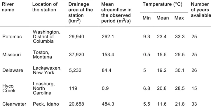
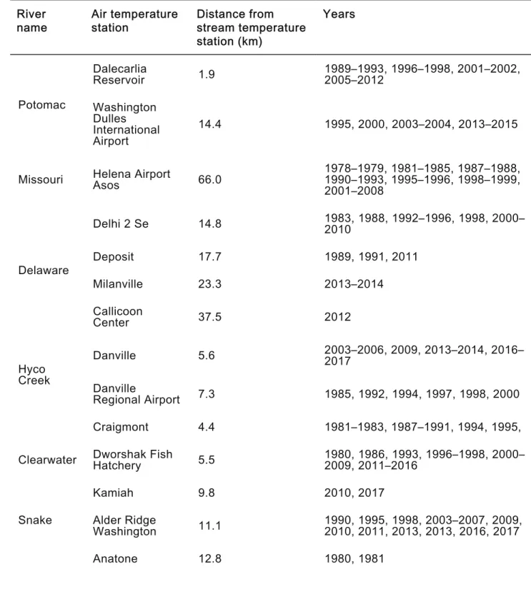
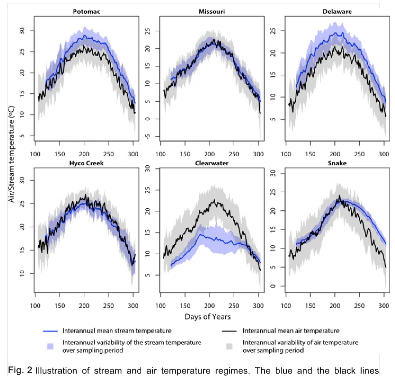
Mean daily stream temperatures were obtained from the U.S. Geological Survey (USGS 2017) on six rivers with long enough records of stream temperatures: Potomac, Missouri, Delaware, Hyco Creek, Clearwater, and Snake rivers (Figure 1). Different instruments were used to record water temperature at the selected study sites. In some cases (Missouri, Delaware, Hyco Creek, Clearwater), thermistors were connected to land‐based dataloggers that recorded water temperature at frequencies varying from 1/15  min to 1/hour. In other rivers (Potomac and Snake), autonomous water quality probes (respectively, DTS and Hydrolab) were deployed. Precision of these instruments varied between ±0.1°C to ±0.5°C. Daily averages were calculated from these data. The drainage areas of the six rivers vary from 119 to 240,765 km (Table 1). For the air temperature, data were obtained from the National Oceanic and Atmospheric Administration (NOAA 2017). For each year of stream temperature records, the air temperature data from the closest meteorological station with complete data in the studied period (less than five missing daily values) were used to produce the air temperature curve for this year. This was repeated for every year until all air temperature curves were produced. Meteorological stations were 1.9–66 km away from the stream temperature stations (Table 2). The resulting stream and air temperature series used in the study are illustrated to show the marked differences in thermal regimes across the six rivers (Figure 2). The QA/QC of temperature time series was performed by the providers of the data. In addition, we visually inspected both air and stream temperature data simultaneously for each year of each river to ensure there was no air exposure of the water temperature data logger. A smoothing of the data also occurred naturally because daily mean values were used as model inputs.

AQ4

Fig. 1 Map of the stream and air temperature stations. The stars show the location of the stream temperature station on each river, whereas the white dots correspond to the air temperature stations used for each river.

Table 1 Stream temperature data used in the study and summary statistics. River

name Location ofthe station Drainagearea at the station (km ) Mean streamflow in the observed period (m /s) Temperature (°C) Number of years available Min Mean Max

Potomac Washington,District of

Columbia 29,940 262.1 9.3 23.4 33.3 25

Missouri Toston,_Montana 37,920 153.4 0.5 15.5 25.5 25

Delaware Lackawaxen,_{New York} 5,232 84.4 5 19.2 30.1 26

Hyco Creek

Leasburg, North

Carolina 119 0.9 6.8 20.8 28.5 15

Clearwater Peck, Idaho 20,658 484.3 5.5 11.6 21.8 33

Snake Anatone,_Washington 240,765 1,068.5 8.8 17.5 24.8 27 Note

Stream temperature data were downloaded from the United States Geological Survey website. Summary statistics were also calculated such as mean streamflow and minimum, mean, and maximum stream temperatures in the observed period.

Table 2 Air temperature data used as model predictors for each river. River

name Air temperaturestation Distance fromstream temperature station (km) Years Potomac Dalecarlia Reservoir 1.9 1989–1993, 1996–1998, 2001–2002,2005–2012 Washington Dulles International Airport 14.4 1995, 2000, 2003–2004, 2013–2015

Missouri Helena Airport_Asos 66.0 1978–1979, 1981–1985, 1987–1988,1990–1993, 1995–1996, 1998–1999, 2001–2008 Delaware Delhi 2 Se 14.8 1983, 1988, 1992–1996, 1998, 2000–₂₀₁₀ Deposit 17.7 1989, 1991, 2011 Milanville 23.3 2013–2014 Callicoon Center 37.5 2012 Hyco Creek Danville 5.6 2003–2006, 2009, 2013–2014, 2016–₂₀₁₇ Danville Regional Airport 7.3 1985, 1992, 1994, 1997, 1998, 2000 Clearwater Craigmont 4.4 1981–1983, 1987–1991, 1994, 1995, Dworshak Fish Hatchery 5.5 1980, 1986, 1993, 1996–1998, 2000–2009, 2011–2016 Kamiah 9.8 2010, 2017

Snake Alder Ridge

Washington 11.1 1990, 1995, 1998, 2003–2007, 2009,2010, 2011, 2013, 2013, 2016, 2017

Fig. 2 Lewiston Nez Perce Co Airport 29.9 1982, 1983, 1988, 1991, 1993, 1994, 1996, 1999, 2002, 2015 Note

Air temperature data were downloaded from the National Oceanic and Atmospheric Administration website. For each year of stream temperature for each river, the closest station with complete air temperature data (less than five missing values) was used to construct the air temperature curve for this year.

Illustration of stream and air temperature regimes. The blue and the black lines show, respectively, the interannual mean stream and air temperature. The blue and black shading represent the internannual variability in the temperature series over the sampling period as illustrated by plus and minus one standard error.

RESULTS

Complete Results for the Potomac River Functional Regression Models

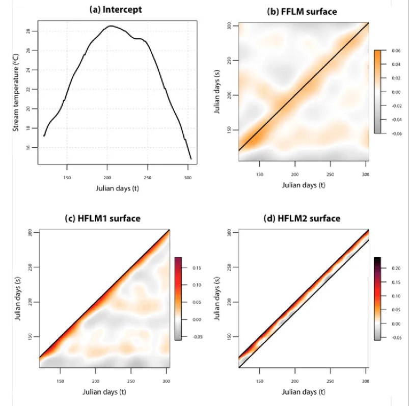
The domain of the stream temperature curves, y(.), is Ω  = [121; 305] days and the domain or air temperature curves, x(.), is Ω  = [106; 305] days, are both limited using Julian days of year. The iterative procedure to fit the functional models (described in Section 2.1) is stopped when the computed RMSE stops decreasing by more than 0.01°C or increases. The intercept α(.) is the same for all models as it represents the smoothed mean functional observation and accounts for seasonality (Figure 3a). β(s,t) surfaces (Figure 3b3d) show the dependence between air temperature at Julian day s (y‐axis) and stream temperature at Julian day t (x‐axis). A positive dependence (in orange to dark red) implies that an increase (or decrease) in air temperature would be associated with an increase (or a decrease) for stream temperature. Negative dependence (in gray) means that a change in the air temperature would be related to a change in the opposite direction for stream temperature. Overall, the β(s,t) surface for the FFLM shows that there is a positive dependence (light orange region in Figure 3b) between air and stream temperature particularly in the range s = t ± 15 days. The stronger dependence (in darker orange) seems to appear around May 20 (Julian day  ≈  145), were β(s,t) is 0.06, which corresponds to the period when the stream temperature shows its greatest increase. For the HFLM1 (Figure 3c), the β(s,t) surface is restricted to the range s < t. The β(s,t) shows a positive dependence between of air and stream temperature in the 15  days before s  =  t. This dependence gets stronger as the line s  =  t is approached. The surface also highlights three particular moments where the surface takes higher values: late May (Julian day ≈ 145), late July (Julian day  ≈  210), and beginning of October (Julian day  ≈  280). For the HFLM2, the surface β(s,t) is restricted to s  ∈  [t, t  –  15] and shows high contribution of air temperature to model stream temperature in all this time range (Figure 3d). For all three models, β(s,t) surface is close to 0 elsewhere, which is expected since air temperature does not typically show high correlation to stream temperature at a lag greater than 15 days. Small negative dependence that sometimes appear in the β(s,t) surfaces (in gray) are negligible as they have low values.

AQ6

1 2

(. )

y¯

Fig. 3 Functional regression coefficients for the Potomac River. (a) shows the functional intercept ɑ(t) which is the same for the three models, (b) the β(s,t) surface of the fully functional linear model (FFLM), (c) the β(s,t) surface of the historical functional linear model 1 (HFLM1), and (d) the β(s,t) surface of the HFLM2. The color scale is the same for the three surfaces to allow easy comparison.

AQ7

The classical RMSE for the Potomac River are 2.05°C, 1.62°C, and 1.45°C, respectively, for the FFLM, HFLM1, and HFLM2 and the NSC are 0.81, 0.88, and 0.90. The bias is below 0.01°C for all three models, but the FFLM has the smallest value (0.0016°C). Concerning the functional

performance criteria (available in Table 4), they are comparable to their classical analogues calculated on a daily basis and will not be described here to avoid redundancy.

Generalized Additive Model

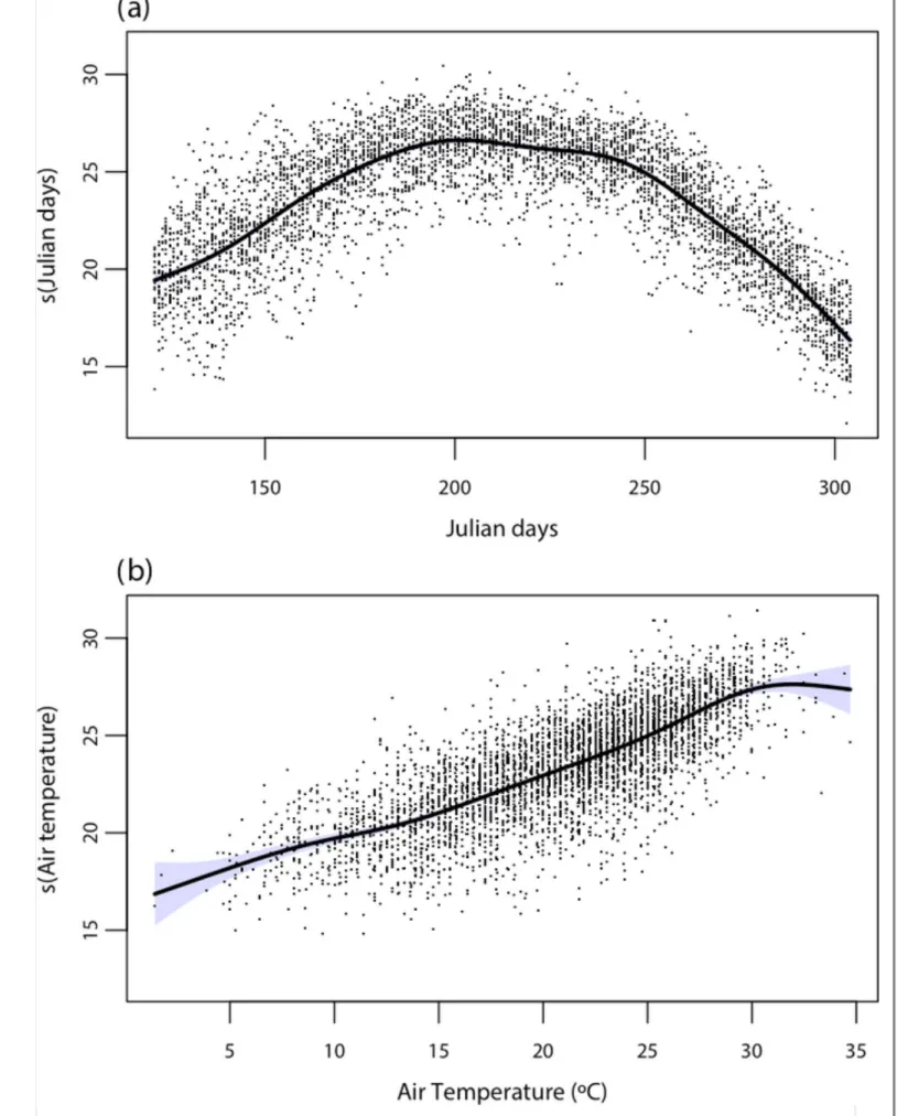
The smooth effect functions for the GAM are obtained from the minimized generalized cross‐ validation (Figure 4). The smooth function of the Julian day of year (Figure 4a) captures the seasonal variation in stream temperature, increasing from May to mid‐July, and then decreasing. The estimated smooth effect function for air temperature (Figure 4b) shows a slight nonlinear relation between air and stream temperature for high‐ and low‐temperature values as mentioned in the introduction. For high air temperatures (>30°C), the effect function becomes steady. In addition, a small change in slope is observed in the 0°C–12.5°C and 12.5°C–30°C ranges. The confidence interval is very narrow for any Julian day of year (cannot be seen on the figure), and it tends to be relatively wide in the extremities of the air temperature effects (<5°C and> 30°C) as there are fewer stream temperature observations in those ranges of values. These effect functions are comparable to the ones obtained by Laanaya et al. (2017) who modeled stream temperature on the Sainte‐Marguerite River (Canada). The RMSE for the GAM is 1.78°C for this river, whereas the NSC is 0.85. Its bias is 0.0003°C with a standard deviation of ±0.89°C.

Fig. 4 Estimated smooth effect functions in the generalized additive model (GAM) for the Potomac River for (a) the Julian day of year and (b) the air temperature.

AQ8

Logistic Model

Optimal parameters are found by minimizing the sum of square errors between simulated and observed stream temperature. The resulting model equation for the Potomac River is:

(14)

While the bias of the LM is comparable to the other models (bias  <  0.1°C), the RMSE is the highest obtained among all the models for the Potomac River (RMSE of 2.57°C). The NSC is also the lowest obtained (NSC of 0.69).

Results Illustration

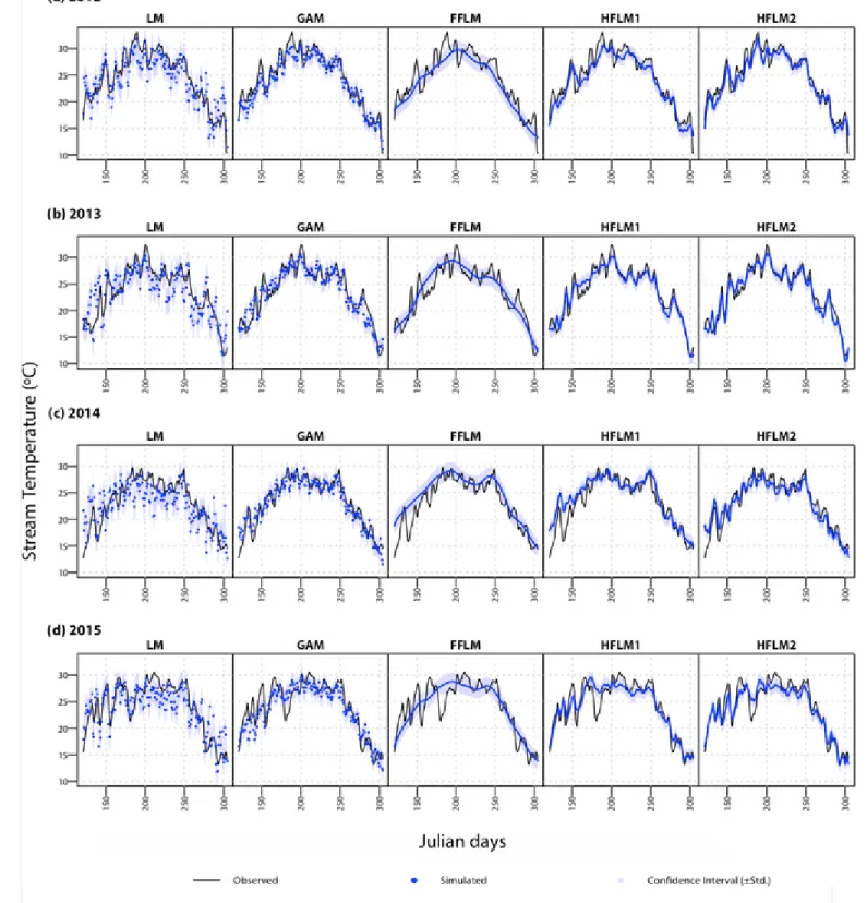
Simulated stream temperatures from the leave‐one‐out procedure and estimated standard deviations are illustrated for the last four years of the Potomac River (Figure 5). For the functional models (FFLM, HFLM1, and HFLM2), a continuous curve of stream temperature is simulated for the entire season. The FFLM simulated well the stream temperature seasonal trend, but underestimated peak temperatures, whereas both the HFLM1 and HFLM2 appear to be better adapted to model minimum and maximum stream temperature than FFLM across the season for the four illustrated years. Results from GAM and LM are plotted as dots as they model discrete values. For these two models, the simulated values vary highly from day to day and do not represent the continuous nature of the stream temperature variable.

=

.

T

42.7463

Fig. 5 Simulated stream temperatures by the leave‐one‐out procedure for the Potomac River. The logistic model (LM) and the GAM simulated multiple daily values (as discrete blue dots) over the studied period, whereas the functional models (FFLM, HFLM1, and HFLM2) simulated a continuous curve (as a continuous blue line). For illustration purpose, only the last four years are shown.

AQ9

For the Missouri River, the RMSE is the lowest for the HFLM2 (1.13°C) followed by the HFLM1 (1.36°C) and the GAM (1.40°C) (Table 3). HFLM2 shows strong improvement compared to the GAM (RMSE difference of −0.27°C), whereas HFLM1 only shows little improvement (RMSE difference = −0.04°C). Regarding the NSC, the same conclusion can be drawn. Bias are below 0.01°C for all models on this river except for the FFLM that has a small positive bias (+0.0301°C).

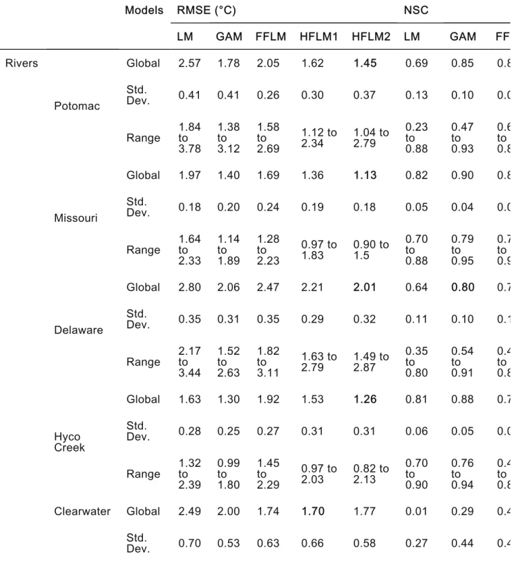
Table 3 Classical performance criteria results.

  Models RMSE (°C) NSC LM GAM FFLM HFLM1 HFLM2 LM GAM FF Rivers Potomac Global 2.57 1.78 2.05 1.62 1.45 0.69 0.85 0.8 Std. Dev. 0.41 0.41 0.26 0.30 0.37 0.13 0.10 0.0 Range 1.84to 3.78 1.38 to 3.12 1.58 to 2.69 1.12 to 2.34 1.04 to2.79 0.23 to 0.88 0.47 to 0.93 0.6 to 0.8 Missouri Global 1.97 1.40 1.69 1.36 1.13 0.82 0.90 0.8 Std. Dev. 0.18 0.20 0.24 0.19 0.18 0.05 0.04 0.0 Range 1.64to 2.33 1.14 to 1.89 1.28 to 2.23 0.97 to 1.83 0.90 to1.5 0.70 to 0.88 0.79 to 0.95 0.7 to 0.9 Delaware Global 2.80 2.06 2.47 2.21 2.01 0.64 0.80 0.7 Std. Dev. 0.35 0.31 0.35 0.29 0.32 0.11 0.10 0.1 Range 2.17to 3.44 1.52 to 2.63 1.82 to 3.11 1.63 to 2.79 1.49 to2.87 0.35 to 0.80 0.54 to 0.91 0.4 to 0.8 Hyco Creek Global 1.63 1.30 1.92 1.53 1.26 0.81 0.88 0.7 Std. Dev. 0.28 0.25 0.27 0.31 0.31 0.06 0.05 0.0 Range 1.32to 2.39 0.99 to 1.80 1.45 to 2.29 0.97 to 2.03 0.82 to2.13 0.70 to 0.90 0.76 to 0.94 0.4 to 0.8 Clearwater Global 2.49 2.00 1.74 1.70 1.77 0.01 0.29 0.4 Std. Dev. 0.70 0.53 0.63 0.66 0.58 0.27 0.44 0.4

For the Delaware River, the LM seems unable to adequately model stream temperature with an RMSE of 2.80°C, whereas the four other models have much lower values. The HFLM2 has the lowest RMSE (2.01°C) followed closely by the GAM (2.06°C). The FFLM and the HFLM have a lower RMSE than the LM, but higher than the GAM. Regarding the NSC, both the GAM and the HFLM2 have the same highest value (0.80), followed by the HFLM1 (0.77), the FFLM (0.71) and the LM (0.64). GAM has the lowest bias across the different models (0.0002°C).

For Hyco Creek, as noted for the Delaware, a small improvement is made in terms of RMSE using the HFLM2 (1.26°C) over the GAM (1.30°C). NSC is also 1% higher for the HFLM2 compared to the GAM. The GAM outperforms the two other functional regression models (FFLM and HFLM1) in terms of RMSE and NSC. Bias is the highest (but still relatively low) for FFLM (+0.0537°C), whereas all other models have bias below 0.01°C for this river. One should also note that the LM performs better than the FFLM on this river.

The Clearwater River obtains satisfying RMSE (below 2°C) for all functional models: 1.74°C, 1.70°C, and 1.77°C for the FFLM, the HFLM1 and the HFLM2, even though the NSC values are relatively low (around 0.45–0.50). For this river, the three functional models are better than both GAM and LM to model daily stream temperatures, in terms of NSC and RMSE. When comparing the functional models, the HFLM1 shows the best performance, followed by the FFLM and then the HFLM2. It is the only river where the HFLM2 does not outperform the other functional regression models.

Finally, for the Snake River, the lowest RMSE is obtained by the HFLM2 (1.10°C), followed by the HFLM1 (1.13°C), the GAM (1.17°C), and the FFLM (1.19°C). The same conclusion is drawn when comparing the NSC. The LM seems to be not adapted for this river with a high value of RMSE (2.87°C) and low NSC (0.46). Finally, again the models have low bias (<0.01°C), except the FFLM and the HFLM1 that both have a positive bias of, respectively, 0.0413°C and 0.0412°C.

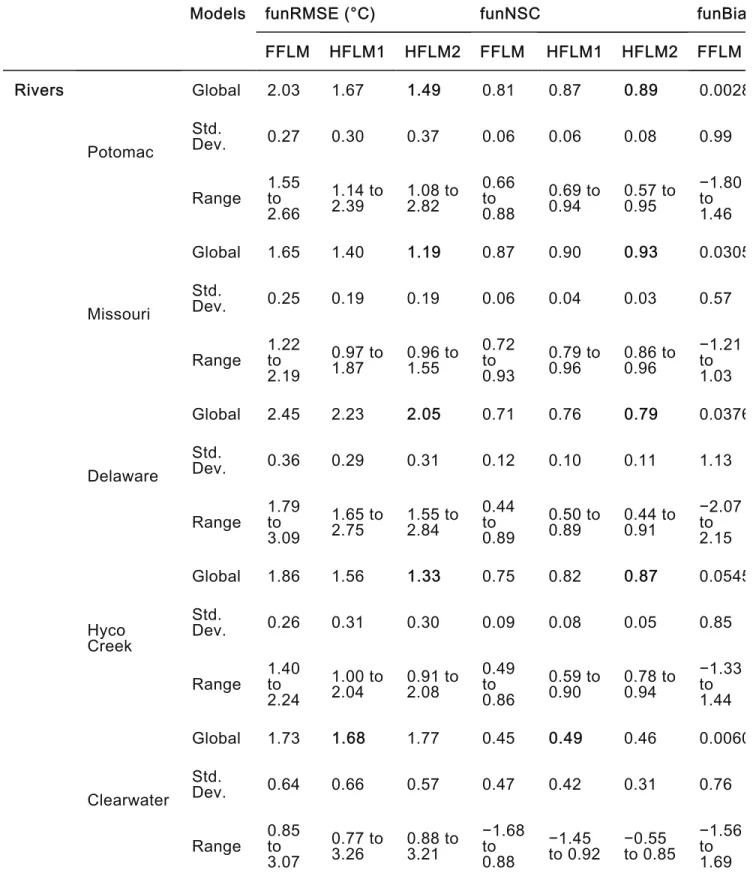
The functional performance criteria are then calculated (Table 4). Conclusions drawn from these criteria are similar to the ones drawn above from classical criteria: the HFLM2 outperforms the

Range 1.64to 4.70 1.23 to 3.71 0.86 to 3.07 0.78 to 3.25 0.87 to3.20 −0.65 to 0.38 −1.35 to 0.78 −1 to 0.8 Snake Global 2.87 1.17 1.19 1.13 1.10 0.46 0.90 0.8 Std. Dev. 0.35 0.35 0.38 0.41 0.36 0.16 0.08 0.0 Range 2.26to 3.97 0.69 to 2.23 0.74 to 2.23 0.58 to 2.20 0.69 to2.30 −0.06 to 0.61 0.66 to 0.97 0.5 to 0.9 Note

The bold and green background indicate which model performed the best when looking at root mean square error (RMSE) and Bias (lowest values) and Nash–Sutcliffe coefficient (NSC) (highest value). The Bias must not be used for comparison purpose here because all values are below the precision of the record instruments of 0.1°C–0.5°C.

two other functional models for all rivers in terms of functional RMSE and NSC, except for the Clearwater River. For this river, the HFLM1 and the FFLM both have lower RMSE (respectively, of 1.68°C and 1.73°C) than the HFLM2 (RMSE of 1.77°C). The NSC is higher for the HFLM1 (0.49) than the HFLM2 (0.46), but lower for the FFLM (0.45). The functional bias is lower for the HFLM2 for all rivers.

Table 4 Functional performance criteria results.

  Models funRMSE (°C) funNSC funBia

FFLM HFLM1 HFLM2 FFLM HFLM1 HFLM2 FFLM Rivers Potomac Global 2.03 1.67 1.49 0.81 0.87 0.89 0.0028 Std. Dev. 0.27 0.30 0.37 0.06 0.06 0.08 0.99 Range 1.55to 2.66 1.14 to 2.39 1.08 to2.82 0.66 to 0.88 0.69 to 0.94 0.57 to0.95 −1.80 to 1.46 Missouri Global 1.65 1.40 1.19 0.87 0.90 0.93 0.0305 Std. Dev. 0.25 0.19 0.19 0.06 0.04 0.03 0.57 Range 1.22to 2.19 0.97 to 1.87 0.96 to1.55 0.72 to 0.93 0.79 to 0.96 0.86 to0.96 −1.21 to 1.03 Delaware Global 2.45 2.23 2.05 0.71 0.76 0.79 0.0376 Std. Dev. 0.36 0.29 0.31 0.12 0.10 0.11 1.13 Range 1.79to 3.09 1.65 to 2.75 1.55 to2.84 0.44 to 0.89 0.50 to 0.89 0.44 to0.91 −2.07 to 2.15 Hyco Creek Global 1.86 1.56 1.33 0.75 0.82 0.87 0.0545 Std. Dev. 0.26 0.31 0.30 0.09 0.08 0.05 0.85 Range 1.40to 2.24 1.00 to 2.04 0.91 to2.08 0.49 to 0.86 0.59 to 0.90 0.78 to0.94 −1.33 to 1.44 Clearwater Global 1.73 1.68 1.77 0.45 0.49 0.46 0.0060 Std. Dev. 0.64 0.66 0.57 0.47 0.42 0.31 0.76 Range 0.85to 0.77 to 0.88 to −1.68to −1.45 −0.55 −1.56to

DISCUSSION

Overall, the HFLM2 seems to be the best performing model compared to the others, with both lowest RMSE and highest NSC on five rivers among six (Potomac, Missouri, Delaware, Hyco Creek, and Snake). For the case of the Clearwater River, the HFLM2 is less performant than the HFLM1 and the FFLM (higher NSC and lower RMSE), but still more performant than the LM and the GAM. The HFLM1 is the best model for one river and the second best on three of the six rivers. The FFLM is outperformed by the GAM for all rivers except for the Clearwater River, but it outperforms the LM on all rivers except for Hyco Creek. However, the LM is generally inappropriate to simulate daily stream temperatures from air temperature data, with higher RMSE and lower NSC compared to other models. In fact, the LM is more suitable for weekly data, as the daily stream temperature have greater autocorrelation (Mohseni et al. 1998; Caissie et al. 2001; Mohseni et al. 2003).

The fact that the FFLM was outperformed by the two other functional models may be attributable to its over parameterization and covering the estimation of the effect in the whole time range including where the effect is clearly negligible. Indeed, by comparing the β(s,t) surface of functional models, the surface is only defined on s < t for the HFLM1 and in s ∈ [t, t – 15] for the HFLM2, reducing the overfitting that can result from using the FFLM with relatively few years used as functional observations. This can be better confirmed on Hyco Creek River where the performance of the FFLM is the lowest since only 15 functional observations were available (compared to 25 and more for the other rivers). With the HFLM2, the functional model with fewest parameters (parsimonious), the results on this river were better than all other models despite the low number of observations. Furthermore, in the case of modeling stream temperature from air temperature data, both the HFLM1 and the HFLM2 would be preferred from a meteorological point of view, as the air temperature at s can only affect the stream temperature if s < t, which is not the case for the FFLM.

Among the six rivers studied, the Delaware and the Clearwater rivers have the worst result in terms of RMSE and NSC. Both the Delaware and the Clearwater River have thermal regimes that vary a lot across the different years compared to the other rivers, as shown by the size of the standard deviation, especially the Clearwater River (Figure 2). It appears that a lag between air and stream temperature exists for this river. This may explain why the GAM and the LM did not perform well on this river compared to the three functional models. The fact that the complete air temperature curve is used as input for functional models may help to model stream

Snake Global 1.17 1.13 1.10 0.89 0.90 0.91 0.0418 Std. Dev. 0.39 0.42 0.37 0.09 0.10 0.08 0.79 Range 0.72to 2.23 0.58 to 2.30 0.68 to2.24 0.56 to 0.97 0.53 to 0.98 0.66 to0.97 −1.75 to 1.98 Note

The bold and green background indicate which model performed the best when looking at funRMSE and funBias (lowest values) and funNSC (highest value). The funBias must not be used for

comparison purpose here because all values are below the precision of the record instruments of 0.1°C–0.5°C.

temperature on rivers like the Clearwater that show a lag between air and stream temperature and may be influenced by other anthropogenic activities (like the presence of a dam in the case of Clearwater), which results in bad performance for classical models like GAM or LM. The Delaware River is the second smallest watershed of this study (sub‐drainage area at the stream temperature station; Table 1). Our smallest watershed, the Hyco Creek River, obtains good modeling performance, so low performance on the Delaware River may not be related to the size of the sub‐drainage area. Hence, the Delaware River may be impacted by other natural and/or anthropogenic variables like the thermal impact of tributaries, the canopy cover or water abstraction (e.g., for the city of New York). All models achieve RMSE  >  2°C on this river, suggesting that adding more predictors (i.e., streamflow, precipitations, light intensity, etc.) to model the stream temperature should be attempted.

By comparing the results obtained in this study to other models used in the literature, our functional models show encouraging and better results for air‐stream relation. For example, the most performant model, the HFLM2, applied to the Missouri, Potomac, Snake, and Hyco Creek rivers, has RMSE ranging from 1.10°C to 1.45°C and NSC from 0.89 to 0.94. This is comparable and even better for some rivers than the GAM performance on the Sainte‐Marguerite River (e.g., RMSE of 1.36°C and NSC of 0.91, Laanaya et al. 2017). Nonparametric methods, such as the KNN model based on water temperature at t − 1 and t − 2 of St‐Hilaire et al. (2012) applied to the Moisie River (RMSE of 1.57°C), also showed lower performance than the HFLM2 of our study (RMSE lower than 1.57°C for four rivers of the six studied). One should note here that the KNN is based on past stream temperatures, whereas the functional model only relies on air temperature to model stream temperature Also, as we used rivers with longer time series compared to the ones of the Sainte‐Marguerite River or the Moisie River and obtained lower RMSE, this may mean that our results are more robust than the ones above because of the larger size of the dataset we used in our study to evaluate models performance.

In addition to better performance, functional models show clear advantages of modeling a whole curve of temperatures instead of multiple daily simulated values in the other classical models. First, the confidence interval for a complete season of simulated values is constant with respect to time, whereas it typically increases when using time series approach (Box et al. 2015). Second, functional regression leads to a parametric model easier to understand and to interpret compared to nonparametric approaches, often called “black‐box models” such as KNN or artificial neural networks (not compared in this article). Third, the use of air temperature curve as one single functional predictor corrects the problem of collinearity when the air temperatures at different time steps or different aggregations like the mean, maximum or minimum over the season are used in other regression models. However, a limitation of the functional models is that they require several years of data to be calibrated. Our river with the shorter record period (15  years) has obtained the smallest improvement using functional regression instead of classical methods (increase in RMSE of 0.04°C compared to GAM and of 0.42°C compared to LM). However, by reducing the size of the β(s,t) surface with the HFLM1 and the HFLM2, we improved substantially the results of functional models with such a low number of functional observations. If such stream temperature data become more available in the future, and they are expected to be given the increased interest for the thermal regime of rivers (e.g., the NorWeST project in western U.S., Isaak et al. 2017; Isaak, Young, et al. 2018, and the RivTemp project in eastern Canada, Boyer et al. 2016), the functional regression models have the potential to become a very useful tool in stream temperature modeling.

in a fitted functional regression model (in our case, the HFLM2 seems to be the most promising tool) would provide a first rough forecast of the stream temperature for next year (season). Then, as the air temperature is observed and forecasted for a shorter time‐step, we would replace our first estimation by the real observed or operationally forecasted air temperature. This will then adjust the predictions that are made for a different time scales, especially for the short‐term period of 10–15 days, as shown by the functional regression surface. This could be done for a particularly interesting period for commercial or recreational fisheries of thermally sensitive species, for example. This approach can be repeated operationally to provide daily updated predictions of stream temperature curves to managers as the air temperature observation/forecast database is being built. Even though models based on air temperature should not be used to long‐term forecast stream temperature (Arismendi et al. 2014), our results based on a leave‐one‐out validation procedure show potential applicability for at least a one‐year window forecast.

CONCLUSION

In the study presented here, three functional models were compared to two classical approaches to model the stream temperature. The functional models were able to model a complete season of stream temperature as a continuous curve compared to the classical model with multiple daily simulated values. To validate the proposed approach, six rivers were modeled to test the performance of functional models in different scenarios. The FFLM and two types of HFLMs (HFLM1 and HFLM2) were tested and the HFLM2 was found to have a better fit based on classical and functional performance criteria on five of the six rivers. For the last river, the HFLM1 appears to be more adapted due to the lag between air and stream temperature regimes. By comparing the HFLM1 to the GAM, the former was found to have a lower RMSE on four of the six rivers. Hence, functional regression seems to be a promising way to model stream temperature with only one predictor. Besides their conceptual advantages, functional models, and more precisely historical functional models, show better results on daily mean stream temperature modeling compared to classical models. Hence, they may provide reliable estimates of stream temperature over a complete season and ultimately, in forecasting stream temperatures.

DATA AVAILABILITY

All data used in this study are freely available and can be downloaded directly from the NOAA (for air temperatures) and USGS (for stream temperatures) websites (links available in the following references).

ACKNOWLEDGMENTS

The authors wish to acknowledge the financial contribution of Natural Sciences and Engineering Research Council of Canada (scholarship for the lead author) and to the Fonds de recherche du Québec — Nature et technologies (FRQNT). The authors are grateful to the reviewers, the associate editor and the editor‐in‐chief for all their constructive comments and suggestions which improved the quality of the paper.

AQ10

Funding Information

Natural Sciences and Engineering Research Council of Canada

Technologies

LITERATURE CITED

Ahmadi‐Nedushan, B., A. St‐Hilaire, T.B. Ouarda, L. Bilodeau, E. Robichaud, N.

Thiemonge, and B. Bobee. 2007. “Predicting River Water Temperatures Using Stochastic Models: Case Study of the Moisie River (Quebec, Canada).” Hydrological Processes 21 (1): 21–34.

Arismendi, I., M. Safeeq, J.B. Dunham, and S.L. Johnson. 2014. “Can Air Temperature Be Used to Project Influences of Climate Change on Stream Temperature?” Environmental Research Letters 9 (8): 084015.

Bel, L., A. Bar‐Hen, R. Petit, and R. Cheddadi. 2011. “Spatio‐Temporal Functional Regression on Paleoecological Data.” Journal of Applied Statistics 38 (4): 695–704. Bélanger, M., N. El‐Jabi, D. Caissie, F. Ashkar, and J. Ribi. 2005. “Estimation de la

température de l'eau de rivière en utilisant les réseaux de neurones et la régression linéaire multiple.” Revue des sciences de l'eau/Journal of Water Science 18 (3): 403–21.

Benyahya, L., D. Caissie, A. St‐Hilaire, T.B. Ouarda, and B. Bobée. 2007. “A Review of Statistical Water Temperature Models.” Canadian Water Resources Journal 32 (3): 179–92. Benyahya, L., A. St‐Hilaire, T.B. Ouarda, B. Bobée, and J. Dumas. 2008. “Comparison of Non‐Parametric and Parametric Water Temperature Models on the Nivelle River, France.” Hydrological Sciences Journal 53 (3): 640–55.

Benyahya, L., A. St‐Hilaire, T.B. Quarda, B. Bobée, and B. Ahmadi‐Nedushan. 2007. “Modeling of Water Temperatures Based on Stochastic Approaches: Case Study of the Deschutes River.” Journal of Environmental Engineering and Science 6 (4): 437–48.

Bernardi, M.S., L.M. Sangalli, G. Mazza, and J.O. Ramsay. 2017. “A Penalized Regression Model for Spatial Functional Data with Application to the Analysis of the Production of Waste in Venice Province.” Stochastic Environmental Research and Risk Assessment 31 (1): 23–38.

Beschta, R., R. Bilby, G. Brown, and L. Holtby. 1987 “Stream Temperature and Aquatic Habitat: Fishery and Forestry Interactions.” In Streamside Management: Forestry and Fishery Interactions, edited by E.O. Salo and T.W. Cundy, 191–232. Seattle: University of Washington, Institute of Forest Resources.

Bjornn, T., and D. Reiser. 1991. “Habitat Requirements of Salmonids in Streams.” American Fisheries Society Special Publication 19 (837): 138.

Bosq, D. 2012. Linear Processes in Function Spaces: Theory and Applications. New York: Springer Science & Business Media.

Boyer, C., A. St‐Hilaire, N. Bergeron, A. Daigle, R. Curry, D. Caissie, and C. Gillis. 2016. “RivTemp: A Water Temperature Network for Atlantic Salmon Rivers in Eastern Canada.” Water News 35: 10–15.

Brockhaus, S., M. Melcher, F. Leisch, and S. Greven. 2017. “Boosting Flexible Functional Regression Models with a High Number of Functional Historical Effects.” Statistics and Computing 27 (4): 913–26.

Brockhaus, S., D. Ruegamer, T. Hothorn, and M.S. Brockhaus. 2017. “Package ‘FDboost’.” https://github.com/boost-R/FDboost.

Brockhaus, S., D. Rügamer, and S. Greven.2017. “Boosting Functional Regression Models with FDboost.” arXiv preprint arXiv:1705.10662.

Brockhaus, S., F. Scheipl, T. Hothorn, and S. Greven. 2015. “The Functional Linear Array Model.” Statistical Modelling 15 (3): 279–300.

Brunner, M.I., D. Viviroli, R. Furrer, J. Seibert, and A.C. Favre. 2017. “Identification of Flood Reactivity Regions via the Functional Clustering of Hydrographs.” Water Resources

Research 54 (3): 1852–67.

Bühlmann, P., and T. Hothorn. 2007. “Boosting Algorithms: Regularization, Prediction and Model Fitting.” Statistical Science 22 (4): 477–505.

Bustillo, V., F. Moatar, A. Ducharne, D. Thiéry, and A. Poirel. 2014. “A Multimodel

Comparison for Assessing Water Temperatures under Changing Climate Conditions via the Equilibrium Temperature Concept: Case Study of the Middle Loire River.” France.

Hydrological Processes 28 (3): 1507–24.

Caissie, D. 2006. “The Thermal Regime of Rivers: A Review.” Freshwater Biology 51 (8): 1389–406.

Caissie, D., N. El‐Jabi, and M.G. Satish. 2001. “Modelling of Maximum Daily Water Temperatures in a Small Stream Using Air Temperatures.” Journal of Hydrology 251 (1): 14–28.

Caissie, D., N. El‐Jabi, and A. St‐Hilaire. 1998. “Stochastic Modelling of Water

Temperatures in a Small Stream Using Air to Water Relations.” Canadian Journal of Civil Engineering 25 (2): 250–60.

Chaouch, M. 2014. “Clustering‐Based Improvement of Nonparametric Functional Time Series Forecasting: Application to Intra‐Day Household‐Level Load Curves.” IEEE Transactions on Smart Grid 5 (1): 411–19.

Chebana, F., C. Charron, T.B. Ouarda, and B. Martel. 2014. “Regional Frequency Analysis at Ungauged Sites with the Generalized Additive Model.” Journal of Hydrometeorology 15 (6): 2418–28.

Chebana, F., S. Dabo‐Niang, and T.B. Ouarda. 2012. “Exploratory Functional Flood Frequency Analysis and Outlier Detection.” Water Resources Research 48 (4). https://doi.org/10.1029/2011WR011040.

Chenard, J.F., and D. Caissie. 2008. “Stream Temperature Modelling using Artificial Neural Networks: Application on Catamaran Brook, New Brunswick.” Canada. Hydrological

Processes 22 (17): 3361–72.

Chiou, J.‐M. 2012. “Dynamical Functional Prediction and Classification, with Application to Traffic Flow Prediction.” The Annals of Applied Statistics 6: 1588–614.

Ciarleglio, A., E. Petkova, T. Tarpey, and R.T. Ogden. 2016. “Flexible Functional

Regression Methods for Estimating Individualized Treatment Rules.” Stat 5 (1): 185–99. Cluis, D.A. 1972. “Relationship between Stream Water Temperature and Ambient Air Temperature.” Hydrology Research 3 (2): 65–71.

Crisp, D., and G. Howson. 1982. “Effect of Air Temperature upon Mean Water Temperature in Streams in the North Pennines and English Lake District.” Freshwater Biology 12 (4): 359–67.

Cuevas, A., M. Febrero, and R. Fraiman. 2002. “Linear Functional Regression: The Case of Fixed Design and Functional Response.” Canadian Journal of Statistics 30 (2): 285–300. Dabo‐Niang, S., and F. Ferraty. 2008. Functional and Operatorial Statistics. New York: Springer Science & Business Media.

DeWeber, J.T., and T. Wagner. 2014. “A Regional Neural Network Ensemble for Predicting Mean Daily River Water Temperature.” Journal of Hydrology 517: 187–200.

Falah, F., S. Ghorbani Nejad, O. Rahmati, M. Daneshfar, and H. Zeinivand. 2017. “Applicability of Generalized Additive Model in Groundwater Potential Modelling and Comparison Its Performance by Bivariate Statistical Methods.” Geocarto International 32 (10): 1069–89.

Ferraty, F., and P. Vieu. 2006. Nonparametric Functional Data Analysis: Theory and Practice. New York: Springer Science & Business Media.

Freund, Y., R. Schapire, and N. Abe. 1999. “A Short Introduction to Boosting.” Journal‐ Japanese Society for Artificial Intelligence 14 (771–780): 1612.

Gervini, D. 2015. “Dynamic Retrospective Regression for Functional Data.” Technometrics 57 (1): 26–34.

Grbić, R., D. Kurtagić, and D. Slišković. 2013. “Stream Water Temperature Prediction Based on Gaussian Process Regression.” Expert Systems with Applications 40 (18): 7407– 14.

Handeland, S.O., A.K. Imsland, and S.O. Stefansson. 2008. “The Effect of Temperature and Fish Size on Growth, Feed Intake, Food Conversion Efficiency and Stomach Evacuation Rate of Atlantic Salmon Post‐Smolts.” Aquaculture 283 (1): 36–42.

Hastie, T., and R. Tibshirani. 1990. Generalized Additive Models. Wiley Online Library. Hedger, R.D., L.E. Sundt‐Hansen, T. Forseth, O. Ugedal, O.H. Diserud, Å.S. Kvambekk, and A.G. Finstad. 2013. “Predicting Climate Change Effects on Subarctic–Arctic Populations of Atlantic Salmon (Salmo salar).” Canadian Journal of Fisheries and Aquatic Sciences 70 (2): 159–68.

Holsinger, L., R.E. Keane, D.J. Isaak, L. Eby, and M.K. Young. 2014. “Relative Effects of Climate Change and Wildfires on Stream Temperatures: A Simulation Modeling Approach in a Rocky Mountain Watershed.” Climatic Change 124 (1–2): 191–206.

Iddrisu, W.A., K.S. Nokoe, A. Luguterah, and E.O. Antwi. 2017. “Generalized Additive Mixed Modelling of River Discharge in the Black Volta River.” Open Journal of Statistics 7 (4): 621. Isaak, D.J., C.H. Luce, D.L. Horan, G.L. Chandler, S.P. Wollrab, and D.E. Nagel. 2018. “Global Warming of Salmon and Trout Rivers in the Northwestern US: Road to Ruin or Path Through Purgatory?” Transactions of the American Fisheries Society 147 (3): 566–87. Isaak, D.J., C.H. Luce, B.E. Rieman, D.E. Nagel, E.E. Peterson, D.L. Horan, S. Parkes, and G.L. Chandler. 2010. “Effects of Climate Change and Wildfire on Stream Temperatures and Salmonid Thermal Habitat in a Mountain River Network.” Ecological Applications 20 (5): 1350–71.

Isaak, D.J., S.J. Wenger, E.E. Peterson, J.M. Ver Hoef, D.E. Nagel, C.H. Luce, S.W. Hostetler, J.B. Dunham, B.B. Roper, and S.P. Wollrab. 2017. “The NorWeST Summer Stream Temperature Model and Scenarios for the Western US: A Crowd‐Sourced Database and New Geospatial Tools Foster a User Community and Predict Broad Climate Warming of Rivers and Streams.” Water Resources Research 53 (11): 9181–205.

Isaak, D., S. Wollrab, D. Horan, and G. Chandler. 2012. “Climate Change Effects on Stream and River Temperatures across the Northwest US from 1980–2009 and Implications for Salmonid Fishes.” Climatic Change 113 (2): 499–524.

Isaak, D.J., M.K. Young, C. McConnell, B.B. Roper, E.K. Archer, B. Staab, C. Hirsch, D.E. Nagel, M.K. Schwartz, and G.L. Chandler. 2018. “Crowd‐Sourced Databases as Essential Elements for Forest Service Partnerships and Aquatic Resource Conservation.” Fisheries 43 (9): 423–30.

Ivanescu, A.E., A.‐M. Staicu, F. Scheipl, and S. Greven. 2015. “Penalized Function‐on‐ Function Regression.” Computational Statistics 30 (2): 539–68.

Janssen, P., and P. Heuberger. 1995. “Calibration of Process‐Oriented Models.” Ecological Modelling 83 (1–2): 55–66.

Jeppesen, E., and T.M. Iversen. 1987. “Two Simple Models for Estimating Daily Mean Water Temperatures and Diel Variations in a Danish Low Gradient Stream.” Oikos 49 (2): 149–55.

Johnson, S.L. 2003. “Stream Temperature: Scaling of Observations and Issues for Modelling.” Hydrological Processes 17 (2): 497–99.

Jourdonnais, J., R. Walsh, F. Pickett, and D. Goodman. 1992. “Structure and Calibration Strategy for a Water Temperature Model of the Lower Madison River.” Montana. Rivers 3 (3): 153–69.

Kaushal, S.S., G.E. Likens, N.A. Jaworski, M.L. Pace, A.M. Sides, D. Seekell, K.T. Belt, D.H. Secor, and R.L. Wingate. 2010. “Rising Stream and River Temperatures in the United States.” Frontiers in Ecology and the Environment 8 (9): 461–66.

Kelleher, C., T. Wagener, M. Gooseff, B. McGlynn, K. McGuire, and L. Marshall. 2012. “Investigating Controls on the Thermal Sensitivity of Pennsylvania Streams.” Hydrological Processes 26 (5): 771–85.

Kim, K., D. Şentürk, and R. Li. 2011. “Recent History Functional Linear Models for Sparse Longitudinal Data.” Journal of Statistical Planning and Inference 141 (4): 1554–66.

Kwak, J., A. St‐Hilaire, and F. Chebana. 2017. “A Comparative Study for Water Temperature Modelling in a Small Basin, the Fourchue River, Quebec.” Canada. Hydrological Sciences Journal 62 (1): 64–75.

Laanaya, F., A. St‐Hilaire, and E. Gloaguen. 2017. “Water Temperature Modelling:

Comparison between the Generalized Additive Model, Logistic, Residuals Regression and Linear Regression Models.” Hydrological Sciences Journal 62 (7): 1078–93.

Larabi, S., A. St‐Hilaire, F. Chebana, and M. Latraverse. 2017. “Multi‐Criteria Process‐ Based Calibration Using Functional Data Analysis to Improve Hydrological Model Realism.” Water Resources Management 32: 195–211.

Lee, R.M., and J.N. Rinne. 1980. “Critical Thermal Maxima of Five Trout Species in the Southwestern United States.” Transactions of the American Fisheries Society 109 (6): 632– 35.

Mackey, A., and A. Berrie. 1991. “The Prediction of Water Temperatures in Chalk Streams from Air Temperatures.” Hydrobiologia 210 (3): 183–89.

Maheu, A., D. Caissie, A. St‐Hilaire, and N. El‐Jabi. 2014. “River Evaporation and Corresponding Heat Fluxes in Forested Catchments.” Hydrological Processes 28 (23): 5725–38.

Maheu, A., A. St‐Hilaire, D. Caissie, N. El‐Jabi, G. Bourque, and D. Boisclair. 2016. “A Regional Analysis of the Impact of Dams on Water Temperature in Medium‐Size Rivers in Eastern Canada.” Canadian Journal of Fisheries and Aquatic Sciences 73 (12): 1885–97. Malfait, N., and J.O. Ramsay. 2003. “The Historical Functional Linear Model.” Canadian Journal of Statistics 31 (2): 115–28.

Masselot, P., S. Dabo‐Niang, F. Chebana, and T.B. Ouarda. 2016. “Streamflow Forecasting Using Functional Regression.” Journal of Hydrology 538: 754–66.

Coefficients in Sea‐Ice Covers Near Resolute Passage.” Canada. Annals of Glaciology 56 (69): 147–54.

McLean, M.W., G. Hooker, A.‐M. Staicu, F. Scheipl, and D. Ruppert. 2014. “Functional Generalized Additive Models.” Journal of Computational and Graphical Statistics 23 (1): 249–69.

Meyer, M.J., B.A. Coull, F. Versace, P. Cinciripini, and J.S. Morris. 2015. “Bayesian

Function‐on‐Function Regression for Multilevel Functional Data.” Biometrics 71 (3): 563–74. Mohseni, O., H.G. Stefan, and J.G. Eaton. 2003. “Global Warming and Potential Changes in Fish Habitat in US Streams.” Climatic Change 59 (3): 389–409.

Mohseni, O., H.G. Stefan, and T.R. Erickson. 1998. “A Nonlinear Regression Model for Weekly Stream Temperatures.” Water Resources Research 34 (10): 2685–92.

Morin, G., J.‐P. Fortin, and J.‐P. Lardeau. 1981. “Modèle CEQUEAU: manuel d'utilisation.” INRS‐Eau, rapport scientifique No 93, 449 pp.

Morrill, J.C., R.C. Bales, and M.H. Conklin. 2005. “Estimating Stream Temperature from Air Temperature: Implications for Future Water Quality.” Journal of Environmental Engineering 131 (1): 139–46.

Morris, J.S..2015. “Functional regression.” Annual Review of Statistics and Its Application 2: 321–59.

Morrison, J., M.C. Quick, and M.G. Foreman. 2002. “Climate Change in the Fraser River Watershed: Flow and Temperature Projections.” Journal of Hydrology 263 (1): 230–44. Nash, J.E., and J.V. Sutcliffe. 1970. “River Flow Forecasting through Conceptual Models Part I—A Discussion of Principles.” Journal of Hydrology 10 (3): 282–90.

Neter, J., M.H. Kutner, C.J. Nachtsheim, and W. Wasserman. 1996. Applied Linear Statistical Models. Chicago: Irwin.

NOAA. 2017. National Centers for Environmental Information. https://www.ncdc.noaa.gov/cdo-web/.

Pilgrim, J.M., X. Fang, and H.G. Stefan. 1998. “Stream Temperature Correlations with Air Temperatures in Minnesota: Implications for Climate Warming.” Journal of the American Water Resources Association 34 (5): 1109–21.

Piotrowski, A.P., M.J. Napiorkowski, J.J. Napiorkowski, and M. Osuch. 2015. “Comparing Various Artificial Neural Network Types for Water Temperature Prediction in Rivers.” Journal of Hydrology 529: 302–15.

Preud'homme, E.B., and H.G. Stefan. 1992. Relationship between water temperatures and air temperatures for Central US Streams. Report No. 333, University of Minnesota, St. Anthony Falls Hydraulic Laboratory, 132 pp.

Quenouille, M.H. 1949. “Approximate Tests of Correlation in Time‐Series.” Journal of the Royal Statistical Society: Series B (Methodological) 11 (1): 68–84.

R Core Team. 2017. R Language Definition. Vienna, Austria: R Foundation for Statistical Computing.

Rahman, A., C. Charron, T.B. Ouarda, and F. Chebana. 2018. “Development of Regional Flood Frequency Analysis Techniques Using Generalized Additive Models for Australia.” Stochastic Environmental Research and Risk Assessment 32 (1): 123–39.

Ramsay, J. 1982. “When the Data are Functions.” Psychometrika 47 (4): 379–96. Ramsay, J.O. 2006. Functional Data Analysis. Wiley Online Library.

Ramsay, J.O., G. Hooker, and S. Graves. 2009. Functional Data Analysis with R and MATLAB. New York: Springer Science & Business Media.

Requena, A.I., F. Chebana, and T.B. Ouarda. 2018. “A Functional Framework for Flow‐ Duration‐Curve and Daily Streamflow Estimation at Ungauged Sites.” Advances in Water Resources 113: 328–40.

Rieman, B.E., D. Isaak, S. Adams, D. Horan, D. Nagel, C. Luce, and D. Myers. 2007. “Anticipated Climate Warming Effects on Bull Trout Habitats and Populations across the Interior Columbia River Basin.” Transactions of the American Fisheries Society 136 (6): 1552–65.

Segura, C., P. Caldwell, G. Sun, S. McNulty, and Y. Zhang. 2015. “A Model to Predict Stream Water Temperature across the Conterminous USA.” Hydrological processes 29 (9): 2178–95.

Sigholt, T., and B. Finstad. 1990. “Effect of Low Temperature on Seawater Tolerance in Atlantic Salmon (Salmo salar) Smolts.” Aquaculture 84 (2): 167–72.

Stefan, H.G., and E.B. Preud'homme. 1993. “Stream Temperature Estimation from Air Temperature.” Journal of the American Water Resources Association 29 (1): 27–45. St‐Hilaire, A., T.B. Ouarda, Z. Bargaoui, A. Daigle, and L. Bilodeau. 2012. “Daily River Water Temperature Forecast Model with a k‐Nearest Neighbour Approach.” Hydrological Processes 26 (9): 1302–10.

Suhaila, J., A.A. Jemain, M.F. Hamdan, and W.Z.W. Zin. 2011. “Comparing Rainfall Patterns between Regions in Peninsular Malaysia via a Functional Data Analysis Technique.” Journal of Hydrology 411 (3–4): 197–206.

Sullivan, K., and T.N. Adams. 1991. “The Physics of Stream Heating: An Analysis of Temperature Patterns in Stream Environments Based on Physical Principles and Field Data.” Weyerheauser Technical Report 044–5002·90/2. Technology Center, Tacoma, WA.