HAL Id: tel-01306953
https://pastel.archives-ouvertes.fr/tel-01306953
Submitted on 25 Apr 2016HAL is a multi-disciplinary open access archive for the deposit and dissemination of sci-entific research documents, whether they are pub-lished or not. The documents may come from teaching and research institutions in France or abroad, or from public or private research centers.
L’archive ouverte pluridisciplinaire HAL, est destinée au dépôt et à la diffusion de documents scientifiques de niveau recherche, publiés ou non, émanant des établissements d’enseignement et de recherche français ou étrangers, des laboratoires publics ou privés.
Nelle Varoquaux
To cite this version:
Nelle Varoquaux. Inferring the 3D architecture of the genome. Bioinformatics [q-bio.QM]. Ecole Nationale Supérieure des Mines de Paris, 2015. English. �NNT : 2015ENMP0059�. �tel-01306953�
T
H
E
S
E
Doctorat ParisTech
TH`
ESE
pour obtenir le grade de docteur d´elivr´e par
l’´
Ecole nationale sup´
erieure des
mines de Paris
Sp´
ecialit´
e doctorale “Bio-informatique”
pr´esent´ee et soutenue publiquement par
Nelle Varoquaux
le 3 d´ecembre 2015
Inferring the 3D structure of the genome.
Inf´erence de la structure tri-dimensionelle du g´enome.
Directeur de th`ese : Jean-Philippe Vert
Jury
M. Emmanuel Barillot, Directeur de Recherche Pr´esident M. William S. Noble, Professor Examinateur M. Marc Marti-Renom, Research Professor Rapporteur M. Julien Mozziconacci, Maˆıtre de conf´erences Examinateur M. St´ephane Robin, Directeur de Recherche Rapporteur M. Jean-Philippe Vert, Directeur de Recherche Examinateur
MINES ParisTech
Centre de Bio-Informatique (CBIO) 35 rue Saint-Honor´e, 77300 Fontainebleau, France
The structure of DNA, chromosomes and genome organization is a topic that has fasci-nated the field of biology for many years. Most research focused on the one-dimensional structure of the genome, studying the linear organizations of genes and genomes and their link with gene expression and regulation, splicing, DNA methylation, . . . . Yet, spa-tial and temporal three-dimensional (3D) genome architecture is also thought to play an important role in many genomic functions.
Chromosome conformation capture (3C) based methods, coupled with next generation sequencing (NGS), allow the measurement, in a single experiment, of genome wide phys-ical interactions between pairs of loci, thus enabling to unravel the secrets behind 3D or-ganization of genomes. These new technologies have paved the way towards a systematic and genome wide analysis of how DNA folds into the nucleus and opened new avenues to understanding many biological processes, such as gene regulation, DNA replication and repair, somatic copy number alterations and epigenetic changes. Yet, 3C technologies, as any new biotechnology, now poses important computational and theoretical challenges for which mathematically well grounded methods need to be developped.
In this thesis, we attempt to address some of the challenges faced while analysing such data.
The first chapter is dedicated to developping a robust and accurate method to infer a 3D model of the genome from Hi-C data. Previous methods often formulated the inference as an optimization problem akin to multidimensional scaling (MDS) based on an ad hoc conversion of contact counts into euclidean wish distances. Chromosomes are modeled with a beads-on-a-string model, and the methods attempt to place the beads in a 3D euclidean space to fullfill a number of, often non convex, constraints and such that the pairwise distances between beads are as close as possible to the corresponding wish distances. These approaches rely on dubious hypotheses to convert contact counts into wish distances, challenging the accuracy of the final 3D model. Another limitation is the MDS formulation which is only intuitively motivated, and not grounded on a clear statistical model. To alleviate these problems, our method models contact counts as a Poisson distribution where the intensity is a decreasing function of the spatial distance between elements interacting. We then formulate the 3D structure inference as a maximum likelihood problem. We demonstrate that our method infers robust and stable models across resolutions and datasets.
The second chapter focuses on the genome architecture of the P. falciparum, a small parasite responsible for the deadliest and most virulent form of human malaria. This
in the complex life cycle of the parasite. In collaboration with the Le Roch lab and the Noble lab, we built 3D models of the genome at three time points which resulted in a complex genome architecture indicative of a strong association between the spatial genome and gene expression.
The last chapter tackles a very different question, also based on 3C-based data. Ini-tially developped to probe the 3D architecture of the chromosomes, Hi-C and related techniques have recently been re-purposed for diverse applications: de novo genome as-sembly, deconvolution of metagenomic samples and genome annotations. We describe in this chapter a novel method, Centurion, that jointly infers the locations of all cen-tromeres in a single yeast genome from Hi-C data, using the cencen-tromeres’ tendency to strongly colocalize in the nucleus. Indeed, centromeres are essential for proper chro-mosome segregation, yet, despite extensive research, centromere locations are unknown for many yeast species. We demonstrate the robustness of our approach on datasets with low and high coverage on well annotated organisms. We then predict centromere coordinates for 6 yeast species that currently lack those annotations.
During the course of my PhD, I have collaborated on several other projects, for which my contributions were minor and thus which I will not describe in the main part of this manuscript. The corresponding papers can be found in appendix. The first project consists in the development of a complete pipeline to preprocess Hi-C data from reads to normalized contact counts. I have worked on a fast and memory efficient python implementation of the normalization. Despite its simplicity, it is to our knowledge the fastest implementation existing so far. The second paper is a review of the epigenetics of the P. falciparum following our first paper on the 3D structure of this parasite. The last project extends the Hi-C protocol to detect interactions between triplets and quadruplets of loci in addition to the usual pairwise interactions. My contribution to this last paper is the development of a method to infer the 3D structure of polyploid method which we applied to the KBM7 nearly haploid human cell line.
La structure de l’ADN, des chromosomes et l’organisation du g´enome sont des sujets fascinants du monde de la biologie. La plupart de la recherche s’est concentr´ee sur la structure unidimensionnelle du g´enome, ´etudiant comment les g`enes et les chromosomes sont organis´es, et le lien entre l’organisation unidimensionnelle et la r´egulation des g`enes, l’´epissage, la m´ethylation, . . . Cependant, le g´enome est avant tout organis´e dans un espace euclidien tridimensionnel, et cette structure 3D, bien que moins ´etudi´ee, joue, elle aussi, un rˆole important dans la fonction g´enomique de la cellule.
La capture de la conformation des chromosomes (3C) et les m´ethodes qui en sont d´eriv´ees, associ´ees au le s´equen¸cage `a haut d´ebit (NGS) mesurent d´esormais en une seule exp´erience des interactions physiques entre paire de loci sur tout le g´enome, permettant ainsi aux chercheurs de d´ecouvrir les secrets de l’organisation des g´enomes. Ces nouvelles technologies ouvrent la voie `a des ´etudes syst´ematiques et globales sur le repliement de l’ADN dans le noyau ainsi qu’`a une meilleure ´etude et compr´ehension de beaucoup de processus biologiques, comme la r´egulation des g`enes, la replication et la r´eparation de l’ADN, les alt´erations du nombre de copies somatiques ainsi que les changements ´epig´en´etiques. Cependant, ces nouvelles m´ethodes 3C, comme toute nouvelle technolo-gie, sont accompagn´ees de nombreux d´efis computationnelles et th´eoriques.
Dans cette th`ese, nous cherchons `a relever un certain nombre de ces d´efis.
Le premier chapitre est d´edi´e au d´eveloppement d’une m´ethode robuste et pr´ecise pour inf´erer un mod`ele tridimensionnel `a partir de donn´ees Hi-C. Les m´ethodes d´evelopp´ees pr´ec´edemment formulent souvent ce probl`eme d’inf´erence comme un probl`eme d’optimisation bas´e sur le positionnement multidimensionnel (en anglais multidimensional scaling) (MDS), reposant sur une d´erivation ad hoc des fr´equences d’interaction en distances euclidiennes. Les chromosomes sont mod´elis´es comme des colliers de perles, lesquels doivent ˆetre plac´es dans un espace euclidien de dimension 3 de telle sorte `a non seulement respecter un cer-tain nombre de contraintes (souvent non convexes) mais aussi de mani`ere `a positionner les perles de fa¸con `a ce que les distances entre elles soient les plus proches des dis-tances d´eriv´ees des fr´equences d’interaction. Ces approches reposent sur des hypoth`eses contestables pour transformer fr´equences d’interaction en distances euclidiennes, soule-vant ainsi un doute sur la validit´e du mod`ele final obtenu. Une autre limitation de ces m´ethodes est la formulation du probl`eme d’inf´erence sous forme MDS, justifi´ee non pas par un mod`ele statistique, mais uniquement par l’intuition. Pour pallier ces probl`emes, notre m´ethode mod´elise les fr´equences d’interaction comme une distribution de Pois-son dont l’intensit´e est une fonction de la distance euclidienne entre paires de loci :
plus stables selon les donn´ees et les r´esolutions de celles-ci.
Le deuxi`eme chapitre est consacr´e `a l’´etude de l’architecture du P. falciparum, un petit parasite responsable de la forme la plus virulente et mortelle de la malaria. Ce projet, dont l’objectif ´etait avant tout de r´epondre `a une question biologique, cherchait `a com-prendre comment l’architecture 3D du g´enome du P. falciparum est li´ee `a l’expression et la r´egulation des g`enes `a diff´erent moments du cycle cellulaire du parasite. En collabora-tion avec les ´equipes de Karine Le Roch et de William Noble, sp´ecialis´ees respectivement dans l’´etude du P. falciparum, et dans le d´eveloppement de m´ethode computationnelle pour ´etudier, entre autre, la structure 3D du g´enome, nous avons construit des mod`eles de l’organisation du g´enome `a trois moments du cycle cellulaire du parasite. Ceux-ci r´ev`elent que le g´enome est repli´e dans le noyau dans une structure complexe, o`u de nombreux nombreux ´el´ements g´enomiques colocalisent: centrom`eres, t´elom`eres, ADN ribosomal, famille de g`enes, . . . Cette architecture indique une forte association entre l’organisation spatiale du g´enome et l’expression des g`enes.
Le dernier chapitre r´epond `a une question tr`es diff´erente, mais aussi li´e `a l’´etude des donn´ees 3C. Celles-ci, initialement d´evelopp´ees pour ´etudier la structure tridimension-nelle du g´enome, ont ´et´e r´ecemment utilis´ees pour des applications tr`es diverses: l’assemblage de g´enomes de novo, la d´econvolution d’´echantillons m´etag´enomiques et l’annotation de g´enomes. Nous d´ecrivons dans ce chapitre une nouvelle m´ethode, Centurion, qui inf`ere conjointement la position de tous les centrom`eres d’un organisme, en utilisant la pro-pri´et´e qu’ont les centrom`eres `a colocaliser dans le noyau. Cette m´ethode est donc une alternative aux m´ethodes de d´etection de centrom`eres classiques, qui, malgr´e des ann´ees de recherche et un enjeu ´economique certain, n’ont pu identifier la position des cen-trom`eres dans un certain nombre d’esp`eces de levure. Nous d´emontrons dans ce projet la robustesse et la pr´ecision de notre approche sur des jeux de donn´ees `a haute comme `a basse couverture. Nous pr´edisons par ailleurs la position des centrom`eres dans 6 esp`eces qui n’avaient pour l’instant aucune annotation.
J’ai par ailleurs au cours de ma th`ese travaill´e sur un certain nombre de projets pour lesquels ma contribution a ´et´e mineure et que je ne d´ecrirai pas dans ce manuscript, mais dont les papiers peuvent ˆetre trouv´es en appendice. Le premier projet consiste au d´eveloppement d’un nouvel outil permettant le pre processing des donn´ees Hi-C afin de construire et de normaliser les cartes de fr´equences d’interaction `a partir des donn´ees brutes de s´equen¸cage. Ma contribution a ´et´e l’impl´ementation en python d’une version optimis´ee `a la fois en m´emoire et en temps de calcul de la normalisation. Cette impl´ementation, bien que tr`es simple et non parall´elis´ee, est `a notre connaissance la
troisi`eme papier ´etend la m´ethode Hi-C afin de d´etecter, en plus des paires d’interactions, des interactions entre trois et quatre ´el´ements. Ma contribution `a ce dernier projet a ´et´e le d´eveloppement d’une m´ethode permettant l’inf´erence de la structure 3D de g´enomes polyplo¨ıdes.
First I would like to express my deep gratitude to Jean-Philippe Vert for supervising my work and sharing his expertise during these three years, for having welcomed me in his research team and giving me the opportunity to work in two prestigious and stimulating institutes: Institut Curie and Mines ParisTech. I would also like to thank William Noble for suggesting the subject and the collaborations from which my PhD relied on, and mentoring me during the past three years.
I would like to thank St´ephane Robin and Marc Marti-Renom for accepting to review my thesis, and sharing interesting comments and discussions with me. I am also grateful to Emmanuel Barillot, William Noble and Julien Mozziconacci for accepting to be part of the jury.
Many people have contributed, directly or indirectly to the work presented in this thesis, and I would like to thank them here: Nicolas Servant, for whom I am grateful for his availablity to answer my questions, for sharing his expertise on Hi-C; Karine Le Roch and the amazing people from her team, Sebastiaan Le Bol and Evelien Bunnik, for providing the collaboration, support and ideas behind our project on P. falciparum, once again William Noble and members of his team, Ferhat Ay, Kate Cook and Wenxiu Hu, for their expertise on the analysis of the 3D structure of the genome and our fruitful collaborations; and all my other collaborators: ´Edith Heard, ´Eric Viara, Chong-Jian Chen, Job Dekker, Bryan Lajoie, Jacques Prudhomme, Maitreya Dunham, Ivan Liachko, Jay Shendure, Josh Burton. I’d like to thank all the members and former members of the CBIO: Alice Schoenauer-Sebag for sharing her experience (and frustration) on using the High Performance Ressources at our disposal, but also her passion for the op´era; Toby Hocking and Anne-Claire Haury, without whom the CBIO was just not quite the same; Elsa Bernard, Erwan Scornet, V´eronique Stoven for all the stories shared around a coffee, Thomas Walter, Yunlong Jiao, Chlo´e Azencott, Matahi Moarii, Pierre Chiche, Xiwei Zhang, Victor Bellon, Judith Ab´ecassis, Svetlana Gribkhova, Nino Shervashidze, Andrea Cavagnino, ´Emile Richard, ´Edouard Pauwels, Kevin Vervier, Olivier Collier, and Azadeh Khaleghi.
I’d like to thank my parents supporting with me during those three years, my brother Ga¨el for convincing me to start my studies again to deepen my knowledge of machine learning.
Abstract iii
R´esum´e v
Acknowledgements viii
1 Introduction and related work 1
§ 1 Peeking under the hood of genome architecture . . . 2
§ 1.1 3C, 4C, 5C and Hi-C data . . . 2
§ 2 The study of chromosome organization . . . 4
§ 2.1 DNA as a polymer . . . 4
§ 2.2 The inference of DNA three-dimensional models . . . 7
§ 3 Long range interactions . . . 9
§ 3.1 De novo genome assembly, haplotype resolution and metagenomic sample deconvolution . . . 10
§ 3.2 Genome annotations and centromeres identification. . . 11
§ 4 Contributions of the thesis. . . 12
2 Inferring the 3D structure of the genome 14 § 1 Introduction. . . 16 § 2 Approach . . . 19 § 2.1 Data normalization . . . 19 § 2.2 MDS-based methods . . . 20 § 2.2.1 Metric MDS . . . 20 § 2.2.2 Nonmetric MDS (NMDS) . . . 21 § 2.3 Poisson model . . . 22
§ 2.4 Default contact-to-distance transfer function . . . 23
§ 2.5 Data . . . 24
§ 2.6 Structure similarity measures . . . 25
§ 3 Results. . . 26
§ 3.1 Simulated Hi-C data . . . 26
§ 3.1.1 Performance as a function of SNR . . . 26
§ 3.1.2 Metric versus nonmetric methods: robustness to incor-rect parameter estimation. . . 29
§ 3.2 Real Hi-C data . . . 29
§ 3.2.1 Stability to enzyme replicates. . . 30
§ 3.2.2 Stability to resolution . . . 30
§ 4 Discussion and conclusion . . . 32
3 Genome architecture of the P. falciparum genome 33 § 1 Introduction. . . 35
§ 2 Results. . . 37
§ 2.1 Assaying genome architecture of P. falciparum at three stages us-ing Hi-C . . . 37
§ 2.2 Three-dimensional modeling recapitulates known organizational principles of Plasmodium genome . . . 38
§ 2.3 Virulence gene clusters on different chromosomes colocalize in 3D . 40 § 2.4 Highly transcribed rDNA units colocalize in 3D during the ring stage . . . 41
§ 2.5 Transcriptionally active trophozoite stage exhibits an open chro-matin structure . . . 43
§ 2.6 Plasmodium genome architecture cannot be explained by volume exclusion . . . 44
§ 2.7 VRSM gene clusters form domain-like structures . . . 45
§ 2.8 Expression is highly concordant with 3D localization for Plasmod-ium genes . . . 47
§ 3 Discussion . . . 48
§ 4 Methods . . . 51
§ 4.1 Experimental protocols . . . 51
§ 4.1.1 P. falciparum strain and culture conditions . . . 51
§ 4.1.2 Cross-linking . . . 51
§ 4.1.3 Tethered conformation capture procedure . . . 51
§ 4.1.4 DNA-FISH . . . 52
§ 4.2 Computational methods . . . 52
§ 4.2.1 Mapping and filtering of sequence data . . . 52
§ 4.2.2 Calculating noise level and percentage of long range con-tacts. . . 53
§ 4.2.3 Aggregating data relative to 10 kb windows. . . 53
§ 4.2.5 Estimating power-law fits to intrachromosomal contact
probabilities . . . 54
§ 4.2.6 Assigning statistical significance to normalized contact maps . . . 54
§ 4.2.7 Identifying stage-specific contacts . . . 55
§ 4.2.8 Inferring the 3D structures . . . 55
Wish distances: . . . 55
Optimization: . . . 56
Initialization: . . . 57
Measuring similarities between structures: . . . 57
Clustering the population of structures: . . . 57
Choosing the parameter β:. . . 57
§ 4.2.9 Eigenvalue decomposition and chromatin compartments . 58 § 4.2.10 Kernel canonical correlation analysis. . . 59
§ 4.2.11 Gene set enrichment analysis . . . 60
§ 4.2.12 Volume exclusion model. . . 60
4 Identification of centromere locations using Hi-C 64 § 1 Introduction. . . 66
§ 2 Method . . . 68
§ 2.1 Single organism Hi-C data . . . 68
§ 2.2 Metagenomic Hi-C data . . . 68
§ 2.3 Assembling the K. wickerhamii genome . . . 70
§ 2.4 Data normalization . . . 70
§ 2.5 Centromere calling . . . 70
§ 2.6 Initializing the optimization problem . . . 71
§ 2.7 Measuring the performance . . . 72
§ 3 Results. . . 72
§ 3.1 Validating the method on S. cerevisiae and P. falciparum . . . 72
§ 3.2 Resolution, sequencing depth and prediction accuracy . . . 75
§ 3.3 Centromere calls on a metagenomic dataset . . . 76
§ 3.4 The effect of the choice of restriction enzyme . . . 78
§ 4 Discussion . . . 79
§ 5 Funding . . . 81
§ 6 Acknowledgements . . . 81
5 Discussion 82
1 Tethered conformation capture procedure protocol . . . 134 Day 1 . . . 134 Day 2 . . . 134 Day 3 . . . 135 Day 4 . . . 135 Day 5 . . . 135 Day 6 . . . 136
2 Assigning statistical significance to normalized contact maps . . . 136
3 DNA-FISH protocol . . . 137
4 Volume exclusion modeling . . . 138
B Supplementaries for Varoquaux et al. [2015] 140 C HiC-Pro: An optimized and flexible pipeline for Hi-C data processing169 § 1 Introduction. . . 170
§ 2 Methods . . . 172
§ 2.1 HiC-Pro Workflow . . . 172
§ 2.2 Quality Controls . . . 174
§ 2.3 Speed and scalability. . . 176
§ 2.4 Contact maps storage . . . 176
§ 2.5 Allele specific analysis . . . 177
§ 3 Results. . . 177
§ 3.1 HiC-Pro results and performances . . . 177
§ 3.2 Implementation of the iterative correction algorithm . . . 180
§ 3.3 Allele specific contact maps . . . 181
§ 4 Conclusion . . . 182
§ 4.1 Supplementary table . . . 185
D Identifying multi-locus chromatin contacts in human cells using teth-ered multiple 3C 187 § 1 Background . . . 188
§ 2 Results. . . 192
§ 2.1 Tethered multiple chromatin conformation capture (TM3C) . . . . 192
§ 2.2 TM3C reveals multi-locus chromatin contacts . . . 193
§ 2.3 Two-phase mapping rescues contacts informative of genome archi-tecture. . . 196
§ 2.4 TM3C data confirms chromatin compartments and topological do-mains . . . 196
§ 2.6 Verification of triples involving IGF2-H19 locus. . . 199
§ 2.7 Three-dimensional modeling of KBM7 genome recapitulates known organizational principles of human cells . . . 201
§ 3 Discussion . . . 203
§ 4 Conclusion . . . 205
§ 5 Materials and methods . . . 205
§ 5.1 TM3C library generation . . . 205
§ 5.2 First phase mapping of sequence data . . . 206
§ 5.3 Second phase mapping of non-mapped reads . . . 207
§ 5.4 Normalization of contact maps . . . 208
§ 5.5 Eigenvalue decomposition . . . 209
§ 5.6 Topological domain analysis . . . 209
§ 5.7 Contacts among regions with the same compartment label . . . 209
§ 5.8 Contacts among regions with similar numbers of DHSs . . . 210
§ 5.9 Contacts within the same topological domain . . . 210
§ 5.10 Inference of the 3D structure . . . 210
§ 6 List of abbreviations used . . . 212
§ 7 Tables . . . 212
§ 8 Supplementary Figures. . . 214
§ 9 Supplementary Tables . . . 225
§ 10 Description of additional data files . . . 226
E Gene regulation via histone modifications, nucleosome positioning and nuclear architecture in P. falciparum 227 § 1 Introduction. . . 228
§ 2 Histone modification landscape of the P. falciparum genome favors eu-chromatin . . . 231
§ 2.1 Post-translational modification of histone proteins . . . 231
§ 2.2 Activating histone marks are abundant and broadly distributed . . 231
§ 2.3 Repressive histone marks are scarce and localized to specific regions233 § 3 Histone variants and nucleosome occupancy are associated with gene ex-pression . . . 235
§ 3.1 Plasmodium exhibits a distinctive nucleosome landscape around coding regions relative to other eukaryotes. . . 235
§ 3.2 Nucleosome dynamics change in concordance with transcriptional activity during the asexual cycle . . . 236
§ 4 Three-dimensional conformation of the P. falciparum genome . . . 237
§ 4.3 Profiling of P. falciparum genome architecture during the asexual
cycle . . . 238
§ 5 A combined model of epigenetic gene regulation in P. falciparum . . . 240
§ 5.1 Nuclear organization and gene regulation . . . 240
§ 5.2 Remodeling of the nuclear organization during the asexual cycle . 242 § 6 Outstanding questions . . . 242
§ 6.1 Clustering of repressive heterochromatin . . . 242
§ 6.2 Mediators of epigenetic control and nuclear remodeling. . . 243
§ 6.3 Epigenetic control in other parasite stages . . . 244
§ 7 Conclusions and prospects . . . 244
Bibliography 248
Supplementary Figures
1 Hi-C Protocol. The procedure relies on cross linking, restriction en-zymes digestions, intra molecular ligation, deproteinization and deep se-quencing. Reads are then aligned to the reference genome, and binned at 10kb, 40kb or 100kb depending on coverage. . . 32 Fractal globule versus the equilibrium globule . . . 6
3 Relationship between contact counts and genomic distances . . . 7
1 Performance evaluation on simulated data, varying the param-eter β. A RMSD of each experiment for varying values of the paramparam-eter β. ChromSDE failed to yield consistent results for 14 experiments (It reported the wrong number of beads in the results file.), and the PM2 al-gorithm failed to converge at the desired precision for one experiment (It exceeded the maximum number of iterations.). B Distance error of each experiment for varying values of β. C Average SNR for each β. Higher SNR corresponds to better quality data. . . 27
2 Performance evaluation for simulated data, varying the
param-eter α. The figure plots the average RMSD of the inferred structures for
a range of α values. As α increases, the SNR of the dataset also increases. 28
3 Predicted structures for chromosome 1 at different resolution Contact counts matrices and predicted structures for the MDS2, NMDS,
PM1 and PM2 methods at 1 Mb (A), 500 kb (B), 200 kb (C), 100 kb (D) 31
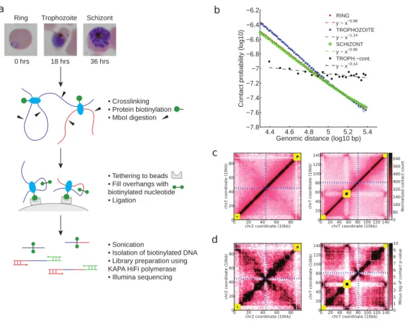
1 Tethered conformation capture of the Plasmodium falciparum
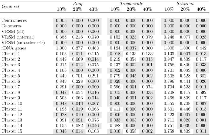
genome. a, Experimental protocol. b, Contact probability as a function of genomic distance, with log-linear fits for the three erythrocytic stages, as well as an experimental control. c, Normalized contact count matrices at 10 kb resolution for chromosome 2 and chromosome 7 in the schizont stage. d, Contact p-values (negative log10 scale) for chromosome 2 and chromosome 7 in the schizont stage. In (c) and (d), yellow boxes denote clusters of VRSM genes, and blue dashed lines indicate the centromere
location. . . 37
2 3D modeling and validation with DNA FISH. a, 3D structures of
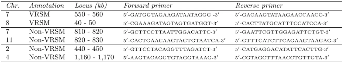
all three stages. The nuclear radii used to model ring, trophozoite and schizont stages were 350, 850, and 425 nm, respectively. Centromeres and telomeres are indicated with light blue and white spheres, respec-tively. Midpoints of VRSM gene clusters are shown with green spheres. b, Validation of colocalization between a pair of interchromosomal loci with VRSM genes (chr7: 550,000 - 560,000 that harbors internal VRSM genes and chr8: 40,000 - 50,000 that harbors subtelomeric VRSM genes) by DNA FISH (left) and by the three-dimensional model for the cor-responding stage (right). The location of the loci in the 3D model is indicated with light blue spheres and pointed by black arrows. c, Vali-dation same as in (b) for a pair of interchromosomal loci that harbor no
VRSM genes (chr7: 810,000 - 820,000 and chr11: 820,000 - 830,000). . . 39
3 Colocalization of highly transcribed rDNA units. Virtual 4C plots
generated at 25 kb resolution using as a bait the A-type rDNA unit on chromosome 7 from crosslinked Hi-C libraries of (a) ring, (b) trophozoite, (c) schizont stages and (d) from the trophozoite control library. Vertical red line indicates the midpoint of the A-type rDNA unit on chromosome 5. Normalized contact counts from 50 kb up- and downstream of the 25 kb bin containing the rDNA unit are used, omitting the rDNA-containing window itself to exclude repetitive DNA. For each window w on chromo-some 5, the contact enrichment is calculated by dividing the contact count between the bait and w to the average interchromosomal contact count
4 Volume exclusion modeling. Observed/expected contact frequency matrices illustrate, for each locus, either the depletion (blue) or enrich-ment (red) of interaction frequencies compared to what would be expected given their genomic distances. a, Observed/expected contact frequency matrices derived from S. cerevisiae chr 7 from volume exclusion modeling (left) and Hi-C data (right). b, Observed/expected matrices from volume exclusion modeling (left) and Hi-C data (right) for P. falciparum chr 7
during the trophozoite stage. . . 45
5 Role of internal VRSM gene clusters in shaping genome
archi-tecture. a-d, Heatmaps of scaled pairwise Euclidean distances derived from the 3D model at 10 kb resolution for (a, b) two chromosomes that harbor internal VRSM gene clusters and (c, d) two chromosomes that
6 Relationship between 3D architecture and gene expression. a,Correlation between expression profiles of pairs of interchromosomal genes as a
func-tion of number of contacts linking the two genes. To generate this plot all interchromosomal gene pairs are first sorted in increasing order of their expression correlation and then binned into 20 equal width quantiles (5th, 10th, ..., 100th). For each bin, the average expression correlation between gene pairs (x-axis) and the average normalized contact count linking the genes in each pair together with its standard error (y-axis) are computed and plotted. Interchromosomal gene pairs that have contact counts within the top 20% for each stage have more highly correlated expression profiles than the remaining gene pairs [Wilcoxon rank-sum test, p-values 2.48e-206 (ring), 0 (trophozoite), and 0 (schizont)]. b, Correlation between expression profiles of pairs of interchromosomal genes as a function of 3D distance between the genes. This plot is generated similar to a but with using 3D distances instead of contact counts (y-axis). In order to summarize results from multiple 3D structures per each stage, we plot the median value among 100 structures with a red line and shaded the region corresponding to the interval between 5th and 95th percentile with gray. Interchromosomal gene pairs closer than 20% of the nuclear diame-ter have more highly correlated expression profiles than genes that are far apart [Wilcoxon rank-sum test, p-values 7.17e-221 (ring), 0 (trophozoite), and 1.57e-88 (schizont)]. c, Gene expression as a function of distance to telomeres. To generate this plot all genes are first sorted by increasing distance to the centroid of telomeres (x-axis) and then binned similar to a into 20 equal width quantiles. The average log expression value [Bunnik et al., 2013] together with its standard error (y-axis) is plotted for genes in each bin. In order to summarize results from multiple 3D structures per each stage, we plot the median value among 100 structures with a red line and shaded the region corresponding to the interval between 5th and 95th percentile with gray. Genes that lie within 20% of the nuclear diameter to the centroid of the telomeres showed significantly lower expression levels [Wilcoxon rank-sum test, p-values 1.54e-12 (ring), 1.69e-32 (trophozoite), 3.37e-20 (schizont)]. d, First kCCA expression profile component score, corresponding to the projection of the gene expression profile onto the
1 Outline of Centurion’s computational workflow 1. Paired-end Hi-C reads are mapped and filtered to produce genome-wide contact maps (see Methods). 2. Contact maps are normalized to correct for technical and experimental biases [Imakaev et al., 2012]. 3. Peaks in marginalized trans contact counts are identified as candidate centromere locations. 4. If necessary, a heuristic reduces the number of centromere candidates that will be used to initialize the joint optimization. 5. A joint opti-mization procedure finds the best set of centromere coordinates, one per chromosome, minimizing the squared distance between the 2D Gaussian fits and the observed trans contact counts. 6. For organisms with known centromere locations, the accuracy of predicted centromere locations is
evaluated; otherwise, the method provides de novo centromere calls. . . . 69
2 Calling centromeres on P. falciparum and S. cerevisiae A. Heatmap
of the normalized trans contact counts for S. cerevisiae Hi-C data at 40 kb overlaid with Centurion’s centromeres calls (black lines). The contact counts were smoothed with a Gaussian filter (σ = 40 kb) for visualiza-tion purposes. White lines indicate chromosome boundaries. B. Per chromosome errors of Centurion’s centromere calls for S. cerevisiae using normalized (black) and raw (blue) Hi-C contact maps at 40 kb resolution. C. Heatmap of trans contact counts for P. falciparum trophozoite data at 40 kb overlaid with Centurion’s centromere calls (dashed black line) and ground truth (red line) for chr 2, 3, 4 and 12. D. Average errors of centromere calls for Centurion (black) and Marie-Nelly et al. [2014b] method for S. cerevisiae data from Duan et al. [2012] and the three stages of P. falciparum when both methods are initialized with the ground truth
centromere coordinates. . . 73
3 Impact of Hi-C library sequencing depth on the stability of the
centromere calls Average variance of the results of Centurion on 500 generated datasets obtained by downsampling the raw contact counts to
the desired coverage. . . 75
4 Centromere calling on a metagenomic sample A. Heatmap of the
trans contact counts for K. wickerhamii overlaid with de novo centromere calls (black lines). The contact counts were smoothed with a Gaussian filter (σ = 40 kb) for visualization purposes. White lines indicate chro-mosome boundaries. B. Box plots indicating the error (in kb) for each chromosome in Centurion’s centromere calls for eight yeasts with known centromere coordinates from the combined metagenomic Hi-C samples
1 Power-law fits to 10 kb aggregated data. . . 101
2 Biases in raw and corrected contact maps for ring stage. . . 102
3 Chromosome visualizations. . . 103
4 Similarity between 3D models inferred from 100 different
ini-tializations. . . 118
5 Clustering of the 100 structures using pairwise RMSD values. . 119
6 Conservation of centromere, telomere and VRSM gene
colocal-izations across 100 different initialcolocal-izations. . . 120
7 3D structures of all three stages (centromere clustering). . . 121
8 Hierarchical clustering of compartment distance matrices. . . . 122
9 Validation of 3D models with DNA FISH. . . 123
10 Clustering of highly transcribed rDNA units in Lemieux et al.
data. . . 124
11 Comparison of inter and intrachromosomal contact prevalence. 125
12 Changes in chromosome territories during the erythrocytic cycle.126
13 Movement of chromosome compartments with respect to each
other. . . 127
14 Volume exclusion modeling and correlation calculation. . . 128
15 Quantification of domain-like behavior of VRSM gene clusters.(a)
Each internal VRSM gene cluster is characterized by a set of strong
intra-cluster contacts (t2) and two sets of contacts with adjacent regions (r5
and r6) that are weak. For comparison, we also consider flanking,
non-VSRM regions of the same size as the original VRSM cluster, including
their “intra-cluster” contacts (t1 and t3) which should be similar to t2 for
a contact map without domain-like structures around VRSM clusters and
contacts with adjacent regions (r4 and r7) which are comparable to (r5
and r6). As seen in this example, a domain-like structure for a VRSM
cluster leads to stronger contacts (+ sign) within t2 compared to both
t1 and t3, and weaker contacts (- sign) within r4 and r7 compared to r5
and r6. (b) The table reports, for each internal VRSM gene cluster and
each stage, the average normalized difference between the intra-cluster contacts within the cluster compared to its two flanking control regions, and similarly for the contacts with adjacent regions. The metric we use for comparing two contact sub-matrices X, Y of dimension N × M is
1 N M PN i=1 PM j=1 xij−yij 1
2(xij+yij) where xij and yij are the ijth entries of X and
Y , respectively. Values that have signs inconsistent with the expected pattern (i.e., +, +, -, -) are indicated with a grey background. Every internal VRSM cluster exhibits the expected sign pattern in at least one
16 Revisiting the relationship between 3D architecture and gene
expression by excluding VRSM genes. . . 131
17 The relationship between distance to the telomeres, nuclear
cen-ter and centromeres versus the gene expression. . . 132
18 kCCA expression profiles component score. . . 133
1 Error on centromere calls for P. falciparum on raw and
normal-ized contact counts (40 kb) . . . 141
2 Error on centromere calls for S. cerevisiae at different
resolu-tions (10 kb, 20 kb, 40 kb) . . . 142
3 Error on centromere calls for P. falciparum at different
resolu-tions (10 kb, 20 kb, 40 kb) . . . 143
4 Centurion vs Marie-Nelly et al. [2014b]’s method . . . 149
5 Pearson correlation matrix of P. falciparum’s chr XII. . . 149
6 Errors on metagenomic sample. . . 152
7 Centromere calls for K. lactis . . . 153
8 Centromere calls for L. kluyveri . . . 154
9 Centromere calls for S. bayanus . . . 155
10 Centromere calls for S. mikatae . . . 156
11 Centromere calls for S. kudriavzevii . . . 157
12 Centromere calls for L. thermotolerans . . . 158
13 Centromere calls for S. pombe . . . 159
14 Centromere calls for Z. rouxii . . . 160
15 Centromere calls for P. pastoris . . . 161
16 Centromere calls for E. gossypii . . . 162
17 Centromere calls for K. wickerhamii . . . 163
18 Centromere calls for L. waltii . . . 164
19 Centromere calls for S. paradoxus . . . 165
20 Centromere calls for S. stipitis . . . 166
1 HiC-Pro workflow. Reads are first aligned on the reference genome. Only uniquely aligned reads are kept and assigned to a restriction fragment. Interactions are then classified and invalid pairs are discarded. If phased genotyping data and N-masked genome are provided, HiC- Pro will align the reads and assign them to a parental genome. These first steps can be performed in parallel for each read chunk. Data from multiple chunks are then merged and binned to generate a single genome-wide interaction map. For allele-specific analysis, only pairs with at least one allele specific read are used to build the contact maps. The normalization is finally
applied to remove Hi-C systematic bias on the genome-wide contact map. 170
2 Read pair alignment and filtering. A. Read pairs are first
indepen-dently aligned to the reference genome using an end-to-end algorithm. Then, reads spanning the ligation junction which were not aligned on the first step are trimmed at the ligation site and their 5’ extremity is re-aligned on the genome. All re-aligned reads after these two steps are used for further analysis. B. Following the Hi-C protocol, digested fragments are ligated together to generate Hi-C products. A valid Hi-C product is expected to involve two different restriction fragments. Read pairs aligned on the same restriction fragment are classified as dangling end or
self-circle products, and are not used to generate the contact maps. . . 173
3 HiC-Pro Quality Controls. Quality controls reported by HiC-Pro
(IMR90, Dixon et al. [2012] data). A. Read pairs statistics after align-ment. Singleton and multiple hits are usually removed at this step. B. Read pairs are assigned to a restriction fragment. Invalid pairs such as dangling-end and self-circle are good indicators of the library quality and are tracked but discarded for subsequent further analysis. C. Fraction of duplicated reads, as well as short range versus long range interactions.
D. Distribution of insert size calculated on a subset of valid pairs. . . 175
4 Comparison of HiC-Pro and hiclib contact maps. Chromosome
6 contact maps generated by hiclib (top) and HiC-Pro (bottom) at dif-ferent resolutions. The chromatin interaction data generated by the two
5 Allele specific analysis. A. Allele specific analysis of GM12878 cell line. Phasing data were gathered from the Illumina Platinum Genomes Project. In total, 2,210,222 high quality SNPs from GM12878 data were used to distinguish both alleles. Around 6% of the read pairs were assigned to each parental allele and used to build the allele-specific contact maps. B. Intra- chromosomal contact maps of inactive and active X chromosome of GM12878 at 500 Kb resolution. The inactive copy of chromosome X is partitioned into two mega-domains which are not seen in the active X chromosome. The boundary between the two mega-domains lies near the
DXZ4 micro-satellite.. . . 181
6 IGV screenshot of BAM file after mapping and fragment
recon-struction. . . 185
7 Correlation of intra and inter-chromosomal contact maps
gen-erated by hiclib and HiC-Pro. . . 186
1 Overview of TM3C experimental protocol and mapping of
paired-end reads to human genome. 1. Cells are treated with formaldehyde, covalently crosslinking proteins to one another and to the DNA. The DNA is then digested with either a single 4-cutter enzyme (DpnII) or a cock-tail of enzymes (AluI, DpnII, MspI, and NlaIII). 2. Melted low-melting agarose solution is added to the digested nuclei to tether the DNA to agarose beads. Thin strings of the hot nuclei plus agarose solution is then transferred to an ice-cold ligation cocktail overnight. 3. After reversal of formaldehyde crosslinks and purification via gel extraction, the TM3C molecules are sonicated and size-selected for 250 bp fragments. 4. Size-selected fragments are paired-end sequenced (100 bp per end) after addi-tion of sequencing adaptors. 5. Each end of paired-end reads are mapped to human reference genome. If both ends are mapped then the pair is considered a double and retained because it is informative for genome architecture. 6. Read ends that do not map to the reference genome are identified and segregated according to the number of cleavage sites they contain for the restriction enzyme(s) used for digestion. 7. Reads with exactly one cleavage site are considered for the second phase of mapping. These reads are split into two from the cleavage site and each of these two pieces are mapped back to the reference genome. 8. Read pairs with either one or both ends not mapped in the first mapping phase are re-considered after second phase. Depending on how many pieces stemming from the original reads are mapped in the second phase, such pairs lead
2 Consistency of TM3C data with known organizational principles and KBM7 karyotype. (a) Number of RE cut sites within reads that are fully mapped and nonmapped in the first phase mapping for KBM7 li-braries. (b) Scaling of contact probability with genomic distance for three crosslinked libraries and one non-crosslinked control library. (c) Scaling of contact probability in log–log scale for three different sets of contacts identified in KBM7-TM3C-1 library. Pairwise chromosome contact ma-trices for (d) KBM7-TM3C-1, (e) KBM7-TM3C-4, (f ) NHEK-TM3C-1 and (g) KBM7-MCcont-4 libraries. For these plots contact counts are averaged over all pairs of mappable 1 Mb windows between the two
chro-mosomes. . . 194
3 Figure 3 - Comparison of TM3C data with existing genome
ar-chitecture datasets Eigenvalue decomposition to identify open/closed chromatin compartments of chromosome 17 (a) from the KBM7 cell line assayed by TM3C and (b) from GM06990 cell line assayed by Hi-C [Lieberman-Aiden et al., 2009]. Topological domain calls and contact count heatmaps of a 6 Mb region of chromosome 6 (c) for the KBM7 cell line assayed by TM3C and (d) for the IMR90 cell line assayed by
Hi-C [Dixon et al., 2012]. . . 197
4 Figure 4 - Genome-wide characterization of triple contacts (a)
Observed over expected percentages of double and triple contacts that link 1 Mb regions with the same (either open or closed) or different (mixed) compartment labels for the KBM7-TM3C-1 library (Methods). Both dou-ble and triple contacts prefer to link open compartments to each other with triples showing slightly more enrichment for this trend. (b) Similar percentages as in (a) but when 1 Mb windows are segregated according to the number of DHSs they contain (Methods). Contacts linking re-gions with higher numbers of DHSs than the median number are enriched within the doubles and the triples of the KBM7-TM3C-1 library. Due to lack of DNase data for KBM7 cells, we use data from six other human cell lines for this analysis. Since the results are very similar among different cell lines, here we only plot the results for K562 which is also a leukemia
5 Figure 5 - Validation of triples using PCR (a) Ten triples extracted from the KBM7-TM3C-1 library that have at least one of their three ends in the 40 kb region surrounding the imprinting control region (ICR) of IGF2 and H19 genes. These triples involve short- and long-range con-tacts within chromosome 11 which are all indicated by tick marks with coordinates in kilobases (kb) displayed only for long-range contacts. In-terchromosomal contacts with other chromosomes are indicated by the chromosome identifier followed by the coordinate in megabases (Mb). Ori-entation of the displayed locus is in the direction of IGF2 and H19 tran-scription. (b) PCR verification of pairwise contacts from triples 3 and 5. One pair of forward/reverse primers is used for each gel (Supplementary
Table 1). . . 200
6 Three-dimensional modeling of KBM7 genome architecture (a)
Three-dimensional structure of the 2 Mb region of chromosome 11 (chr11:1,000,000-3,000,000) which is centered around IGF2-H19 imprinting control
re-gion. This structure is inferred from normalized contact counts of KBM7-TM3C-1 data at 40 kb resolution using the Poisson model from Varoquaux et al. [2014]. (b) Three-dimensional structure of the KBM7 genome, which is haploid for all chromosomes other than diploid chromosome 8 (8A, 8B) and partially diploid chromosome 15 (15A, 15B) (see Methods for details of the 3D inference). Different colors represent different chro-mosomes, and white balls represent chromosome ends. Same 3D structure as (b) when confined to (c) only a subset of long chromosomes, (d) only
a subset of small chromosomes, (e) two small and two large chromosomes. 202
7 Number of restriction enzyme cut sites across the human genome.215
8 Chromosome contact maps of different contacts types for
KBM7-TM3C-1. . . 216
9 Ploidy track for select chromosomes from KBM7 TM3C data. . 217
10 PCR verification of triples 1–10 listed in Main Figure 5. . . 218
11 Additional PCR experiments for triples 5 and 6. . . 219
12 Methylation status of the distal contact partners of IGF2-H19
ICR for triple 1. . . 220
13 Methylation status of the distal contact partners of IGF2-H19
ICR for triple 2. . . 221
14 Methylation status of the distal contact partners of IGF2-H19
ICR for triples 3 and 4. . . 222
15 Gene expression measured by RNA-seq for the IGF2-H19 locus.223
16 Gene-poor chromosome 18 does not colocalize strongly with
1 Overview of the P. falciparum . . . 229
2 Large-scale depletion of the transcriptionally permissive histone variant
H2A.Z and activating histone marks in the telomeric cluster visualized on the 3D P. falciparum genome. ChIP-seq data from Bartfai et al. Bartfai et al. [2010] for four histone variants or marks were downloaded from GEO (accession number: GSE23787) and mapped to the P. falci-parum genome (PlasmoDB v9.0) using the short read alignment mode of BWA (v0.5.9) [Li and Durbin, 2010] with default parameter settings. Reads were post-processed, and only the reads that map uniquely with a quality score above 30 and with at most two mismatches were retained for further analysis. Retained reads were subjected to PCR duplicate elimination and then were aggregated for each non-overlapping 5 kb bin across the P. falciparum genome. The number of reads for each 5 kb bin was normalized using the overall sequencing depth of the corresponding ChIP-seq library. Plotted are the log2 ratios of sequence-depth normal-ized number of reads from the ChIP-seq library versus the correspond-ing input library (red: depletion, blue: enrichment) for A: H2A at 40 hours post invasion (hpi), B: H2A.Z at 10 hpi, C: H2A.Z at 30 hpi, D: H2A.Z at 40 hpi, E: H3K9ac at 40 hpi, and F: H3K4me3 at 40 hpi. 3D models for the ring, trophozoite and schizont stages were generated in Ay et al. [2014b] and were colored with ChIP-seq enrichment/depletion from 10, 20, and 40 hpi, respectively. Light blue and white spheres in-dicate centromeres and telomeres, respectively. The black dashed circle denotes the telomeric cluster for each stage. See Supporting information or http://noble.gs.washington.edu/proj/plasmo-epigenetics for the
rotat-ing 3D figure of each available ChIP-seq library.. . . 233
3 Visualization of ChIP-seq data from Jiang et al. [46] on the 3D
P. falciparum genome at the ring stage. ChIP-seq data from Jiang
et al. for 5 histone marks were downloaded from SRA (accession number: SRP022761) and processed as described in the caption of Figure 2. Due to lack of input libraries from this publication, the input libraries from Bartfai et al. at different time points were pooled into one aggregated input library which is then used for normalization of each Jiang et al. ChIP-seq library. Similar to Figure 2, log2 ratios of ChIP-seq versus in-put were plotted for A: H3K9me3, B: H3K36me3, C: H4K20me3, and D: H3K4me3 at 18 hpi. The 3D model for the ring stage from [Ay et al., 2014b] was used to visualize enrichment/depletion of each histone mark. See http://noble.gs.washington.edu/proj/plasmo-epigenetics for the
blue) and telomeric (red) clusters are localized at the nuclear periphery. Subtelomeric virulence genes (blue) are anchored to the nuclear perimeter and cluster with internally located var genes in repressive center(s), char-acterized by repressive histone marks H3K9me3 and H3K36me3. The sin-gle active var gene (green) is located in a perinuclear compartment away from the repressive center(s). In addition, active rDNA genes (orange) also cluster at the nuclear periphery. The remaining genome (purple) is largely present in an open, euchromatic state with a number of notable features. (i) Nucleosome levels are high in genic and lower in intergenic regions, while gene expression correlates with nucleosome density at the transcription start site. (ii) Intergenic regions are bound by nucleosomes containing histone variants H2A.Z and H2B.Z. (iii) Intergenic regions con-tain H3K4me3, the level of which does not influence transcriptional activ-ity. (iv) H3K9ac is mainly found in intergenic regions and extends into 5’ ends of coding regions, with highly expressed genes showing higher levels of H3K9ac. (v) Active genes are marked with H3K36me3 towards their 3’ end. B: Remodeling of the nuclear organization during the asexual cycle. Extensive remodeling of the nucleus takes place as the parasite progresses through the ring, trophozoite and schizont stages. In the tran-sition from the relatively inert ring stage to the transcriptionally active trophozoite stage, the size of the nucleus and the number of nuclear pores increase, accompanied by a decrease in genome-wide nucleosome levels, resulting in an open chromatin structure that allows high transcription rates. In the schizont stage, the nucleus divides and recompacts, histones are re-assembled and transcription is shut-down, to facilitate egress of the
parasites’ daughter cells and re-invasion of new red blood cells. . . 247
Supplementary Tables
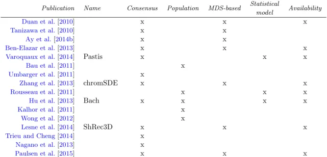
1 A comparison of 3D inference methods . . . 10
1 Stability across enzyme replicates. For each resolution, the table lists the Spearman correlation the two enzyme replicate datasets, and, for each inference method, the average RMSD and Spearman correlation between pairs of structures inferred from the two datasets. Boldface values cor-respond to the best RMSD or correlation values among all five methods. In general, higher resolution leads to a lower correlation between pairs of
inferred structures. . . 30
2 Stability across resolution. The table lists the average RMSD and
Spearman correlation between pairs of structures of different resolutions. In bold are the lowest average RMSD and highest average Spearman correlation. These values were computed on mouse ESC HindIII libraries
Dixon et al. [2012]) . . . 31
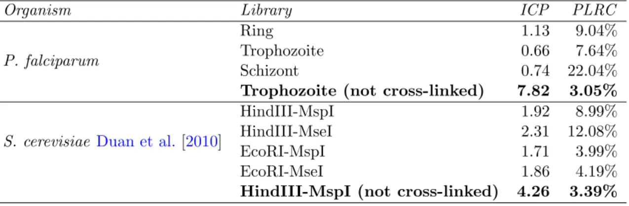
1 Quality measures for Hi-C data. . . 88
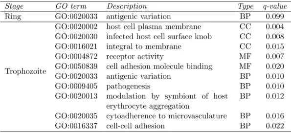
2 GSEA results for genes involved in stage-specific contacts. . . 89
3 Assessing sensitivity of the 3D inference to different parameter
settings. . . 90
4 Assessing sensitivity of the 3D inference to spatial constraints. . 91
5 Colocalization test for 21 gene/locus sets.. . . 92
6 Sequences of primers used for the generation of FISH probes. . . 93
7 Gradient values of the log-linear fits that best capture the
scal-ing of contact probability with genomic distance for each
chro-mosome. . . 94
8 GSEA results for the ring stage on the first component of the
kCCA. . . 95
9 GSEA results for the trophozoite stage on the first component
of the kCCA. . . 96
10 GSEA results for the schizont stage on the first component of
the kCCA. . . 97
11 kCCA enrichment of 15 expression clusters. . . 98
12 GSEA results for the second component of the kCCA. . . 99
13 Density score for varying values of β parameter at different stages.100
1 Centromere calls for S. cerevisiae, ground truth and errors . . . 144
2 Centromere calls for P. falciparum (ring stage), ground truth
and errors . . . 145
3 Centromere calls for P. falciparum (trophozoite stage), ground
4 Centromere calls for P. falciparum (schizont stage), ground
truth and errors . . . 147
5 Centromere calls for A. thaliana, annotation units and errors . . 148
6 M-3D multi-sample statistics for each organism’s contact counts
matrices (20 kb) . . . 150
7 M-Y multi-sample statistics for each organism’s contact counts
matrices (20 kb) . . . 151
8 K. lactis centromere calls, ground truth and errors . . . 153
9 L. kluyveri centromere calls, ground truth and errors . . . 154
10 S. bayanus centromere calls, partial ground truth and errors . . 155
11 S. mikatae centromere calls, ground truth and errors . . . 156
12 S. kudriavzevii centromere calls, ground truth and errors . . . . 157
13 L. thermotolerans centromere calls, ground truth and errors . . 158
14 S. pombe centromere calls, ground truth and errors . . . 159
15 Z. rouxii centromere calls, ground truth and errors . . . 160
16 P. pastoris de novo centromere calls . . . 161
17 E. gossypii de novo centromere calls . . . 162
18 K. wickerhamii de novo centromere calls . . . 163
19 L. waltii de novo centromere calls. . . 164
20 S. paradoxus de novo centromere calls . . . 165
21 S. stipitis de novo centromere calls . . . 166
1 Comparing solutions for Hi-C data processing. HOMER offers several
programs to analysis Hi-C data from aligned reads. HICUP proposes a complete pipeline until the detection of valid interaction products. It can be used together with the SNPsplit software to extract allele specific mapped reads. The hiclib python library can be applied for all anal-ysis steps but requires good programming skills and cannot be used in a single command-line manner. None of these softwares offers to easily process very large data in a parallel mode. The HiCorrector software [Li et al., 2015] provides a parallel implementation of the iterative correction algorithm for dense matrix. Note that HOMER and hiclib also offer ad-ditional functions for downstream analysis. In the case of HiC-Pro, the downstream analysis is supported by the HiTC BioConductor package
[Servant et al., 2012]. . . 171
2 Comparison of contact maps format. Disk space for IMR90 CCL186
genome-wide contact map generated either using the classical dense
3 HiC-Pro performances and comparison with hiclib. HiC-Pro was run on IMR90 Hi-C dataset from Dixon et al. and Rao et al. in order to generate contact maps at resolution 20kb, 40kb, 150kb, 500kb and 1Mb. Contact maps at 5kb were also generated for the IMR90 CCL186 dataset. CPU time for each step of the pipeline is reported and compared to the hiclib python library. The reported results include I/O time of writing
contact maps in text format. . . 178
4 Performances of iterative correction on IMR90 data. HiC-Pro is
based on a fast implementation of the iterative correction algorithm. We therefore compare our method with the HiCorrector software [Li et al.,
2015] for Hi-C data normalization (hours:minutes:seconds). All
algo-rithms were terminated after 20 iterations (see supplementary material
for details). . . 180
5 Comparison of hiclib and HiC-Pro processing steps. . . 185
1 Sequences of primers used for PCR verification.. . . 225
1 Overview of most-studied histone modifications and variants in P.
falci-parum and comparison of their genome-wide distribution or function in
other eukaryotes. . . 234
2 Summary of organizational features of P. falciparum nucleus and genome
at three distinct stages during asexual parasite replication in human red
Introduction and related work
R´esum´e
L’architecture spatiale et temporelle du g´enome joue un rˆole important dans beau-coup de fonctions g´enomiques, mais est cependant `a l’heure actuelle peu comprise. Le d´eveloppement r´ecent du protocol Hi-C, qui permet en une seule exp´erience de mesurer les fr´equences d’interactions entre paire de loci sur tout le g´enome, ouvre la porte `a une ´etude plus syst´ematique de la structure tridimensionnelle du g´enome. Dans ce chapitre, nous introduisons les concepts sous-jacents `a la cap-ture de la conformation des chromosomes, la struccap-ture de l’ADN et aux m´ethodes d’inf´erence de l’architecture 3D du g´enome.
Abstract
The spatial and temporal genome architecture is thought to play an important role in many genomic functions, but is yet poorly understood. Recently, the develop-ment of the Hi-C protocol, which allows in a single experidevelop-ment to assess genome wide physical interactions between pairs of loci, has paved the way for a systematic analysis of the 3D structure of DNA. We aim in this chapter at providing some background on chromosome conformation capture, the structure of DNA and the field of 3D architecture inference.
§ 1
Peeking under the hood of genome architecture
Methods to investigate the 3D structure of the genome fall broadly into two categories: bio imaging techniques and biochemical protocols. In the first category, light microscopy allows single cell visualization of specific loci and enables live cell imaging, sometimes at very high resolution [Cremer and Cremer, 2010]. Yet, these techniques limit studies to a very small number of loci. On the other hand, biochemical protocols, such as chromosome conformation capture (3C) and its derivatives, enable to measure physical interaction between DNA fragments [Dekker et al., 2002], but performing single cell experiments is troublesome, and tracking live cell impossible. To understand how DNA fold into a nucleus, one has to juggle both technologies. In this thesis, we are mostly interested in analysing 3C-based datasets.
§ 1.1 3C, 4C, 5C and Hi-C data
In recent years, the technique of chromosome conformation capture (3C) [Dekker et al.,
2002], which identifies physical contacts between different genomic loci and yields infor-mation about their relative spatial distance in the nucleus, has paved the way for the systematic analysis of the 3D structure of DNA. 3C techniques and its derivatives are based on 5 experimental steps [Lieberman-Aiden et al.,2009,Kalhor et al.,2011].
• Cross-linking : results in the cross-linking of DNA segments to proteins and to cross-linking of proteins with each other (Figure 1-A).
• Restriction digest A restriction enzyme is added in excess to the cross-linked DNA (Figure1-B). The restriction enzyme will cut the DNA at specific nucleotide sequences, separating the non-cross-linked DNA from the cross-linked chromatin. Recognition sequences in DNA differ from each restriction enzyme, producing dif-ferent lengths and sequences of strands. The selection of the restriction enzyme depends on the type of studies targeted in the experiment.
• Intramolecular Ligation The third step is an intramolecular ligation step. DNA fragments are joined together (Figure1-C). There are two major types of ligation junctions: the first is the ligation of two neighboring DNA fragments, and the second is the junction that is formed when ligating one end of the fragment to the other end of the same fragment.
• Reverse Cross-links The fourth step consists of reversing the first step: the reversal of cross-links (Figure 1-D).
Figure 1: Hi-C Protocol. The procedure relies on cross linking, restriction enzymes digestions, intra molecular ligation, deproteinization and deep sequencing. Reads are then aligned to the reference genome, and binned at 10kb, 40kb or 100kb depending on
coverage.
• Quantitation Polymerase chain reaction (PCR) is used to amplify the DNA copies and to assess the frequencies of the fragments of interest, which are then sequenced (Figure1-E).
After paired-end sequencing, each pair of reads can be associated to one [
Lieberman-Aiden et al., 2009] or several [Ay et al.,2015b] DNA interactions. We can then create
a symmetric matrix of integers, for which rows and columns corresponds to a specific genomic window and entries correspond to the number of times locus i and j were observed to contact on another. We denote by C the interaction frequency matrix, and cij the interaction frequency between locus i and locus j.
These protocols are complex, and yield highly biased interaction frequencies [Imakaev
et al.,2012,Cournac et al.,2012,Yaffe and Tanay,2011]. Imakaev et al.[2012] proposes
a simple iterative method, called ICE, to normalize the data. In short, the authors assume that the bias of each entry cij of the matrix can be written as the product
of two biases βi and βj corresponding to biases induced by loci. Hence, we can write
cij = βiβjpij, where pij is the probability of locus i interacting with locus j. Thus,
P
ipij = 1. This is a non convex optimization problem that can be solved exactly by
an iterative process. To avoid degeneracies, we filter out the top 2% sparse loci from our entry matrix before applying ICE (this value needs to be adapted to each dataset). To give an intuition, this method projects each vector of interactions onto the ℓ1 unit
ball. In practice, it yields an expected interaction frequency count: kpij, where k is the
average interaction frequency other all pairs of loci.
Though still quite recent, chromosome conformation capture and its genome wide deriva-tives are now widely used to discover how DNA folds in a bunch of different organisms
[Duan et al., 2010, Sexton et al., 2012, Tanizawa et al., 2010, Ay et al., 2014b]. The
sequencing [Rao et al., 2014, Jin et al., 2013]. As any genome-wide sequencing data, Hi-C usually requires several millions or billions of paired-end sequencing reads, depend-ing on genome size and on the desired resolution. Managdepend-ing these data thus requires optimized bioinformatics workflows able to extract the contact frequencies in reasonable computational time and with reasonable storage requirements. The overall strategy to analyze Hi-C data is converging among recent studies and summarized in Lajoie et al.
[2015]. Our collaborators and we have built HiC-Pro (see Appendix C, an easy-to-use and complete pipeline to process Hi-C data from raw sequencing reads to the normalized contact maps. Once these processing steps are done, one can finally proceed to the study of genome organization and DNA folding from Hi-C data in an attempt to unfold the mysteries of genome architecture.
§ 2
The study of chromosome organization
The study of chromosome organization based on contact count maps broadly falls into two categories: model-based studies and data-driven studies. The former methods con-sider the polymer nature of DNA to leverage the theoretical and computational work done in statistical physics of polymers to build with as few assumptions as possible many chromosome conformations. Those chromosome conformations are then used to compare against experimental data, such as Hi-C contact count matrices, in order to it-eratively improve the models. These models offer mechanistical insights into the folding of DNA. The latter approaches use the experimental data to infer 3D models, by typi-cally minizing a cost function ensuring the models are as consistent as possible with the data. These data driven models and analysis are the primary focus of this thesis.
Though we here review some of the methods used to study and build models, this is a very incomplete view of a blooming field. Rosa and Zimmer[2014] provide a more thorough (but again incomplete) overview of computational models of genome architectures.
§ 2.1 DNA as a polymer
Polymer physics divide homopolymers (polymers with identical monomers) into three main types, which are then extended to build more complex models: (1) the random coil, (2) the swollen coil, (3) the equilibrium polymer. These polymers are characterized by relationships such as the one between the size of a polymer subchain L(s) as a function of its lengths s, between the size of the polymer L(N ) and the total length of this polymer N , or between the contact probability between monomers P (s) and the linear distance
between monomers s. DNA being a polymer, each pair of nucleic acid forms a monomer, and the distance s is the genomic distance between two loci.
The random coil corresponds to an unconstrained polymer, best described by a random walk. A random coil of length N has an expected size of N1/2, and so has any of its
subchain: L(s) ∼ s1/2. The contact probability between two monomers is P (s) ∼ s−3/2. These relationships lead to a low density polymer, where contact between monomers is sparse. The modeling of the random coil does not exclude the volume occupied by monomers: when taking in account that monomers can not occupy the same chain, one obtains a new polymer model known as the swollen coil, best described as a self avoiding random walk. This type of polymer occupies a larger space: L(N ) ∼ N35.
If the polymer is constrained in a small volume, the polymer folds into an equilibrium globule state. This polymer behaves as a random walk, until it bounces of the boundary of the constrained space, and starts another random walk inside the confined volume. The expected size of this polymer is N1/3. The size of a subchain of a polymer follows the relationship: L(s) = s1/2 for s < N2/3 and constant elsewise: it is the same as
a random coil until it plateaus. The probability of contact between two monomers is P (s) = s−3/2for s < N2/3 and constant elsewise: once again, it is the same relationship
as the random coil, until it becomes constant. Interestingly, this polymer is uniformely distributed in the constrained space, and the density of the polymer is independent of the total length N and the volume V .
Another interesting polymer behaviour is the fractal globule: when the chain is suffi-ciently long and the constrained volume suffisuffi-ciently small, the polymer forms knotted crumples of increasing sizes. The polymer is then constrained by the available vol-ume and the volvol-ume it itself occupies, which creates topological constraints forcing the polymer to collapse into crumples. First proposed by Grosberg et al. [1988], and fur-ther analysed by Mirny [2011], the polymer presents interesting properties: the size of any subchain follows the same law as the equilibrium globule, but without the plateau: L(s) ∼ s1/3, and the probability of contact between two monomers is inversely
propor-tional to the linear distance that separates them: P (s) ∼ s−1.
Now that we have briefly summarized the different theoritical behaviour of polymers, let us have a closer look at the relationships we observe in practice, using DNA contact counts maps obtained through Hi-C. From figure 3, we can observe that organisms fall into two categories: the first group, composed of small genomes such as S. cerevisae, P. falciparum, behaves as an equilibrium globule coil, while the second group, composed of large genomes such as mammifer genomes and A. thaliana D. drosophilae, exhibit properties of fractal globules.
Figure 2: Fractal globule versus the equilibrium globule
This image from Mirny [2011] illustrates the difference between the fractal globule or crumpled globule and the equilibrium globule. In the first row, the fractal globule’s subchain occupes a distinct territory in the nucleus, while the second row illustrates the equilibrium globule’s property to occupy a wide space in the nucleus.
104 105 106 107 108 Mean 100 101 102 103 104 V a ri a n ce S. cerevisiae D. melanogaster H. sapiens
Figure 3: Relationship between contact counts and genomic distances
Average contact counts as a function of genomic distance for S. cerevisiae [Duan et al.,
2010], D. melanogaster [Sexton et al.,2012] and chr 1 of the KBM7 human cell line [Rao
et al.,2014]. S. cerevisiae’s genome behaves as a equilibrium globule, whileSexton et al.
[2012]’s D. melanogaster and Rao et al.[2014]’s KBM7 datasets display relationships of the fractal crumpled globule. Notice that S. cerevisiae’s average contact counts decreases more quickly with the genomic distance than D. melanogaster ’s and KBM7’s.
§ 2.2 The inference of DNA three-dimensional models
Several techniques have been developed to infer three-dimensional models of the genome from interaction counts data. They fall into three categories: the first finds an average structure by optimizing an objective function as [Tanizawa et al., 2010, Duan et al.,
2010, Ben-Elazar et al., 2013]. The second samples local minima from a optimization
problem leading to the study of the population of local minima [Bau et al.,2011]. The last samples the posterior distribution [Rousseau et al.,2011].
Tanizawa et al. [2010] model the 3D genome of the fission yeast (3 chromosomes) by a
string of 622 beads, each bead xi being the center of a 20kb section. The first step was
to infer physical distances δij from frequency interactions. They studied eighteen pairs
of genes using FISH measurements, and fitted the Hi-C data on the distances with a non linear regression curve. The second step was to compute the coordinates of the beads, such that the distances between the beads match the inferred physical distances to the best, with additional biological motivated constraints.