HAL Id: pastel-00961962
https://pastel.archives-ouvertes.fr/pastel-00961962
Submitted on 20 Mar 2014HAL is a multi-disciplinary open access
archive for the deposit and dissemination of sci-entific research documents, whether they are pub-lished or not. The documents may come from teaching and research institutions in France or abroad, or from public or private research centers.
L’archive ouverte pluridisciplinaire HAL, est destinée au dépôt et à la diffusion de documents scientifiques de niveau recherche, publiés ou non, émanant des établissements d’enseignement et de recherche français ou étrangers, des laboratoires publics ou privés.
Augmented reality : the fusion of vision and navigation
Nadège Zarrouati-Vissière
To cite this version:
Nadège Zarrouati-Vissière. Augmented reality : the fusion of vision and navigation. Other [cs.OH]. Ecole Nationale Supérieure des Mines de Paris, 2013. English. �NNT : 2013ENMP0061�. �pastel-00961962�
T
H
È
S
E
INSTITUT DES SCIENCES ET TECHNOLOGIES
École doctorale n
O432: Sciences des Métiers de l’Ingénieur
Doctorat ParisTech
T H È S E
pour obtenir le grade de docteur délivré par
l’École Nationale Supérieure des Mines de Paris
Spécialité « Mathématique et Automatique »
présentée et soutenue publiquement par
Nadège Zarrouati-Vissière
le 20 décembre 2013
La réalité augmentée:
fusion de vision et navigation.
Augmented reality:
the fusion of vision and navigation.
Directeur de thèse: Pierre ROUCHON
Jury
M. Tarek HAMEL, Professeur, I3S, Université de Nice-Sophia-Antipolis Rapporteur
M. Gabriel PEYRE,Chargé de recherche, CEREMADE, Université Paris-Dauphine Rapporteur
M. Hisham ABOU-KANDIL, Professeur, MOSS, ENS Cachan Président du jury
M. Jean-Jacques SLOTINE, Professeur, NSL, MIT Examinateur
Mme Karine BEAUCHARD, Chargée de recherches, CMLS, Ecole Polytechnique Examinateur
M. Pierre ROUCHON, Professeur, CAS, MINES ParisTech Examinateur
Nadège Zarrouati-Vissière
Direction Générale de l’Armement 7-9 rue des Mathurins 9220 Bagneux France.
E-mail: [email protected]
Key words. - Augmented reality, navigation systems, vision, SLAM algorithms, bias estimation, depth, observability, differential geometry, MEMS sensors, RGBD data
Mots clés. - Réalité augmentée, systèmes de navigation, vision, algorithmes SLAM, estimation de biais, profondeur, observabilité, géométrie différentielle, capteurs MEMS, données RGBD
Il n’y a pas de vent favorable pour celui qui ne connaît pas son port. Sénèque
Tell me and I forget, teach me and I may remember, involve me and I learn. Benjamin Franklin
Remerciements
Je remercie Hisham Abou-Kandil président du jury, Gabriel Peyré et Tarek Hamel rapporteurs de ma thèse ainsi que les examinateurs Jean-Jacques Slotine, Karine Beauchard, Pierre Rouchon et Mathieu Hillion.
Je tiens à remercier tout particulièrement mon directeur de thèse Pierre Rouchon pour la confiance qu’il m’a faite en me confiant ces travaux de thèse, et pour son attention bienveillante au cours de ces trois années. Cela a été un honneur pour moi de pouvoir travailler à ses côtés et de bénéficier de son recul scientifique.
Je remercie Karine Beauchard pour son enthousiasme et sa réactivité pour répondre avec justesse et compétence à mes diverses questions. J’ai beaucoup apprécié nos séances de travail et nos nombreuses discussions, qu’elles soient d’ordre mathématique ou non.
Je remercie les membres du CAS, en particulier Philippe Martin et Laurent Praly, pour leurs conseils éclairés et leur gentillesse.
Je remercie Jean-Jacques Slotine, venu de loin pour participer au jury de ma thèse, pour m’avoir donné à Boston l’idée et l’envie de faire cette thèse au CAS.
Je remercie mon employeur la DGA pour m’avoir permis de réaliser cette formation par la recherche; je remercie en particulier ma future équipe qui s’est avant même mon arrivée intéressée à mon travail.
Je remercie Sysnav, qui a mis à ma disposition les moyens expérimentaux qui m’ont permis de valider mes travaux théoriques et bien plus encore. J’y ai trouvé une équipe soudée, passionnée par la technique et toujours prête à partager cet enthousiasme, dont les lumières m’ont été précieuses dans le domaine de la navigation inertielle. Je remercie en particulier Mathieu Hillion pour sa constante disponibilité pour répondre à mes questions, Pierre-Jean, Eric et Quentin pour avoir toujours été prêts à m’apporter de l’aide, et Georges pour ses anecdotes et sa longue expérience en navigation.
Je remercie les stagiaires que j’ai eu le plaisir d’encadrer pendant ma thèse, Mian, Rémi et surtout David pour sa gentillesse et sa persévérance.
Enfin, je remercie ma famille: mes parents qui m’ont appris à mener jusqu’au bout mes entreprises, mes soeurs qui m’ont aidée à ne pas les prendre trop au sérieux, et David qui m’a redonné la motivation et la confiance en moi qui parfois me manquaient pour surmonter les difficultés rencontrées.
Augmented reality:
Résumé
Cette thèse a pour objet l’étude d’algorithmes pour des applications de réalité visuellement augmentée. Plusieurs besoins existent pour de telles applications, qui sont traités en tenant compte de la contrainte d’indistinguabilité de la profondeur et du mouvement linéaire dans le cas de l’utilisation de systèmes monoculaires. Pour insérer en temps réel de manière réaliste des objets virtuels dans des images acquises dans un environnement arbitraire et inconnu, il est non seulement nécessaire d’avoir une perception 3D de cet environnement à chaque instant, mais également d’y localiser précisément la caméra. Pour le premier besoin, on fait l’hypothèse d’une dynamique de la caméra connue, pour le second on suppose que la profondeur est donnée en entrée: ces deux hypothèses sont réalisables en pratique. Les deux problèmes sont posés dans le contexte d’un modèle de caméra sphérique, ce qui permet d’obtenir des équations de mouvement invariantes par rotation pour l’intensité lumineuse comme pour la profondeur. L’observabilité théorique de ces problèmes est étudiée à l’aide d’outils de géométrie différentielle sur la sphère unité Riemanienne. Une implémentation pratique est présentée: les résultats expérimentaux montrent qu’il est possible de localiser une caméra dans un environnement inconnu tout en cartographiant précisément cet environnement.
Abstract
The purpose of this thesis is to study algorithms for visual augmented reality. Different requirements of such an application are addressed, with the constraint that the use of a monocular system makes depth and linear motion indistinguishable. The real-time realistic insertion of virtual objects in images of a real arbitrary environment yields the need for a dense Three
dimensional (3D) perception of this environment on one hand, and a precise localization of
the camera on the other hand. The first requirement is studied under an assumption of known dynamics, and the second under the assumption of known depth: both assumptions are practically realizable. Both problems are posed in the context of a spherical camera model, which yields SO(3)-invariant dynamical equations for light intensity and depth. The study of theoretical observability requires differential geometry tools for the Riemannian unit sphere. Practical implementation on a system is presented and experimental results demonstrate the ability to localize a camera in a unknown environment while precisely mapping this environment.
Contents
Introduction 1
Acronyms 5
I From motion to depth 7
1 Camera models and motion equations 9
1.1 Camera models . . . 9
1.1.1 Pinhole model . . . 9
1.1.2 Other models . . . 14
1.2 Spherical model: notations . . . 15
1.3 Motion equations . . . 15
1.3.1 Spherical model: the camera in a fixed environment. . . 15
1.3.2 Pinhole-adapted model . . . 18
2 Formulation as a minimization problem 21 2.1 Variational methods applied to optical flow estimation . . . 21
2.1.1 Optical flow. . . 21
2.1.2 Variational methods applied to inverse problems. . . 22
2.1.3 Variational method with Sobolev prior. . . 23
2.1.4 Variational method with total variation prior. . . 25
2.2 Variational methods applied to depth estimation . . . 27
2.2.1 Estimation of depth with Sobolev priors. . . 27
2.2.2 Estimation of depth by total variation minimization . . . 29
3 Reconstruction of the depth 33 3.1 Asymptotic observer based on optical flow measures . . . 33
3.2 Asymptotic observer based on depth estimation . . . 37
4 Implementations, simulations and experiments 39 4.1 Simulations . . . 39
CONTENTS
4.1.2 Implementation of the depth estimation based on optical flow measures . . 40
4.1.3 Implementation of the asymptotic observer based on rough depth estimation 42 4.2 Experiment on real data . . . 45
II From depth to motion 49 5 Estimation of biases on linear and angular velocities 53 5.1 Statement of the problem . . . 54
5.2 Observability of the reference system . . . 55
5.2.1 Characterization of the observability . . . 55
5.2.2 Scenes with non trivial stationary motion . . . 55
5.3 The asymptotic observer . . . 62
5.3.1 A Lyapunov based observer . . . 62
5.3.2 Decrease of the Lyapunov function . . . 63
5.3.3 Existence and uniqueness . . . 64
5.3.4 Regularity and bounds . . . 64
5.3.5 Continuity . . . 65
5.3.6 Convergence . . . 65
5.4 Practical implementation, simulations and experimental results . . . 67
5.4.1 Adaptation to a spherical cap . . . 67
5.4.2 The observer in pinhole coordinates . . . 69
5.4.3 Simulations . . . 69
5.4.4 Experiments on real data. . . 74
5.5 Proof of the well posedness of the observer . . . 76
5.5.1 Local solutions . . . 76
5.5.2 Bounds on solutions. . . 80
5.5.3 Global solutions . . . 82
5.6 Continuity of the flow . . . 82
6 The geometrical flow method for velocity estimation 85 6.1 The geometrical flow as a conservation law . . . 85
6.2 Implementation of the method for a pinhole camera model . . . 87
6.3 Implementation of the method for a pinhole camera model including radial distortion . . . 89
6.4 Experiments on real data . . . 91
7 Estimation of biases on angular velocity and acceleration 97 7.1 Problem formulation . . . 98 7.2 Observability . . . 98 7.3 Observer design . . . 99 7.4 Asymptotic convergence. . . 100 7.5 Exponential convergence . . . 103 xii
CONTENTS
7.6 Robustness to noise . . . 104
7.7 Implementation on real data . . . 108
III Simultaneous tracking and mapping for augmented reality 115 8 Architecture of the original algorithm 117 8.1 Overview of the algorithm . . . 118
8.2 Map initialization . . . 119
8.3 Pose estimation (tracking) . . . 120
8.4 Mapping . . . 123
8.4.1 Keyframe insertion . . . 123
8.4.2 Bundle adjustment . . . 123
8.5 Relocalisation . . . 125
9 Fusion of magneto-inertial, visual and depth measurements 127 9.1 Sensors and synchronization . . . 128
9.1.1 Depth sensor . . . 128 9.1.2 Magneto-inertial sensors . . . 128 9.1.3 Synchronization . . . 129 9.2 Map initialization . . . 129 9.3 Mapping . . . 129 9.3.1 Keyframe insertion . . . 130
9.3.2 Depth data in bundle adjustment . . . 131
9.4 Pose estimation . . . 131
9.5 Tracking quality and relocalization . . . 132
9.5.1 Assessing the visual tracking quality . . . 134
9.5.2 Relocalization procedure . . . 134
9.6 Localization and augmented reality . . . 135
9.6.1 Attitude estimation . . . 136
9.6.2 Position estimation . . . 137
10 Experimental results 139 10.1 Experimental conditions. . . 139
10.2 Linear velocity, position and attitude estimation . . . 142
10.2.1 Translation along the lateral direction . . . 142
10.2.2 Exploration of an entire room . . . 148
CONTENTS
Conclusion 159
Appendix 163
A Differential geometry on the Riemannian unit sphere 165
A.1 Riemannian manifolds . . . 165
A.2 Differential calculus . . . 166
B Matrix Lie groups and Lie algebra 169 C 3D rigid-body kinematics and quaternions 171 C.1 Attitude and angular velocity . . . 171
C.1.1 The special orthogonal group . . . 171
C.1.2 Quaternions . . . 173
C.1.3 Euler angles . . . 174
C.2 Position, linear velocity and acceleration . . . 175
C.3 The Special Euclidean group . . . 176
Bibliography 179
Introduction
Augmented reality
The emergence of mobile phones since the years 2000, and smartphones in the last few years led to an increasing demand of the public to quick, easy and wide access to personal as well as general information in any situation of everyday’s life. For example, it is nowadays a basic requirement to be able to precisely locate oneself wherever in the world, even although
the Global Positioning System (GPS), based on radio-frequency signals, is well known to be
highly sensitive (among others) to the relative positions of the satellite constellation with respect to the user ([Kaplan and Hegarty, 2005]). Real-time localization is only one example of augmented reality, which can be defined as the addition of intangible information to our physical perception of the world: this can be achieved through sound, vision or even touch
([Azuma et al., 1997]). Numerous applications have been reached by augmented reality: a few
examples are urban navigation ([Graham et al., 2013]), learning ([Gavish et al., 2013]), surgery or medical applications in general ([Speidel et al., 2013] or [Mousavi Hondori et al., 2013]),
3D modeling ([Brenner, 2005], [Yang et al., 2013] or [Newcombe and Davison, 2010]), robots teaching and learning ([Borrero and Marquez, 2013]), manufacturing
([Ong et al., 2008]), archeology ([Girbacia et al., 2013]), fine arts ([Bovcon et al., 2013]), gesture
training ([de Sorbier et al., 2012]), astrophysics ([Vogt and Shingles, 2013]); but also virtual in-terior design ([Han and Seo, 2013]), fashion ([Ruzanka et al., 2013]), tourism ([Lin et al., 2013]), advertisement ([Shiva and Raajan, 2013]), e-commerce ([Li et al., 2013]) and, last but not least, gaming ([Santoso and Gook, 2012] or [Woun and Tan, 2012]).
The most natural and appealing way to augment reality is by the mean of visual addition, which yields some requirements, of software as well as of hardware types. The obvious hardware requirements are a capture (e.g a video camera, now available on most mobile phones
[Khan et al., 2013]), and a display technology: the later has become the last fashion trend with
the overwhelming (but still unavailable for the large public at the time of writing) Google Glass product ([Edwards, 2013] or [Ackerman, 2013]). The hidden hardware technology is the processing capability, which is driven by the software complexity. As for the software part, the possibility to add virtual objects to a real image in a realistic way requires the ability to localize the camera with respect to the visible environment, to inlay a 3D model of the object in the physical world, and to project this3D view in the image. The first part of these requirements is generally solved by Simultaneous Localization and Mapping (SLAM) algorithms: from the
visual input (from one or multiple cameras), which can be aided by inertial inputs present in most portable technologies in the form of Micro-Electro-Mechanical Systems (MEMS) sensors, the camera is localized with respect to a 3D model of the environment. This model can be a complete input, for example a 3D model of the city ([Lothe et al., 2010]); a partial input, e.g fiducial known markers ([Lim and Lee, 2009]); or simply a real-time reconstruction of the environment without any input, which is the domain of application of Structure from Motion
(SfM) algorithms ([Wei et al., 2013]). As for the second part of the software requirements, it
leads to the necessity of a dense 3D modeling of the environment (at the very least a current camera-centered model) to be able to handle occlusions of the virtual object with the real world
([Kahn, 2013] or [Zollmann and Reitmayr, 2012]).
Dense 3D reconstruction of the environment
Environment reconstruction is
tightly related to the SLAM problem [Smith et al., 1990], which can be addressed by nonlinear filtering of observed key feature locations (e.g. [Civera et al., 2008], [Montemerlo et al., 2003]), or by bundle adjustment ([Strasdat et al., 2010b, Strasdat et al., 2010a]). The problem of designing an observer to estimate the depth of single or isolated keypoints has raised a lot of interest, specifically in the case where the relative motion of the carrier is described by constant known ([Abdursul et al., 2004, Dahl et al., 2010]), constant unknown [Heyden and Dahl, 2009], or time varying known ([Dixon et al., 2003, Karagiannis and Astolfi, 2005, Luca et al., 2008,
Sassano et al., 2010]) affine dynamics. From a different perspective, the seminal paper of
[Matthies et al., 1989] performs incremental depth field refining for the whole field of view via
iconic (pixel-wise) linear Extended Kalman filtering. However, estimating a sparse point cloud is insufficient for augmented reality applications, and none of these methods provide an accurate dense depth estimation in a general setting concerning the environment and the camera dynamics.
Motion estimation
For the specific problem of motion estimation and localization, the nature and the quality of the available measurements are critical, and delimit the reachable performances. In the 1950s, expensive Inertial Measurement Units (IMUs) were developed, as missile guidance and control required extremely accurate navigation data [Bezick et al., 2010,Chatfield, 1997,Faurre, 1971]. Tactical grade IMUs, less expensive, enable dead-reckoning techniques over short time periods, but require position fixes provided by GPS[Abbott and Powell, 1999], or combination through data fusion of other sensors outputs [Skog and Handel, 2009,Vissière et al., 2007]. As to recent low-cost IMUs using MEMS technologies, the cumulated error due to the bias of gyroscopes integrated over long time periods induces drift in orientation, which can be bounded. However, from biased accelerometers, only high frequency output can be relied on, since the double integration induces a position error quadratically growing in time; even more severe errors can be induced when accelerometers are used in the frame of attitude estimation. As odometers and velocimeters (e.g. Doppler radar [Uliana et al., 1997], Pitot tube,Electromagnetic (EM) log
sensor), are commonly available technologies in vehicles, mass market applications can combine their linear velocity outputs with angular velocity from low-quality IMUs. Unfortunately, Pitot probes and EM log sensors are known to only provide airspeed and Speed through the
water (STW) instead of Speed over ground (SOG): real-time or beforehand bias estimation is
necessary to make the measurements from these sensors exploitable. In a different category, the Kinect device has been a huge outbreak in the robotics and vision communities as it provides depth measurements registered at each pixel of a RGB image, at a relatively low cost: this output is named RGBD (Red Green Blue and Depth: refers to the aligned pair of
an usual color image and a depth image (RGBD)). This sensor trivially solves the ambiguity
issue in ego-motion estimation by a monocular system: while motion is generally estimated up to as scale factor (for example by homography estimation [Hamel et al., 2011]), RGBDdata provide the input required to solve theSfMproblem without resorting to stereo vision techniques
[Pollefeys et al., 2004,Zhang and Faugeras, 1992].
Layout of the dissertation
Part Iis dedicated to the study of real-time dense3Dreconstruction under the assumptions of known camera motion and known projection model for the on board monocular camera. These assumptions are motivated by the existence of a novel system developed by Sysnav company, providing linear and angular velocity of a system obtained by processing of measurements from gyrometers, accelerometers and magnetometers (see [Vissiere, 2008,Dorveaux, 2011] for a com-plete description and the historical development of this novel technique, and [Vissière et al., 2008] for a technical patented description).1
We propose in this part a new estimation method for dense depth data, from known camera dynamics, namelysix degrees of freedom (6-DOF)inputs. This method is based on a formulation of the optical flow constraint deriving from the spherical camera model introduced in [Bonnabel and Rouchon, 2009], where the camera dynamics is made explicit. This model is described in Chapter 1 and highlighted by a comparison with other camera models. The principal assumptions and notations are also introduced in this chapter. Variational methods applied to this constraint enable dense depth field estimation (Chapter
2). In addition, a so-called geometrical flow constraint can be exploited to design a non-linear observer based on optical flow or depth measurements (Chapter3). These results are based on
[Zarrouati et al., 2012a, Zarrouati et al., 2012b, Zarrouati et al., 2012c], and meet the needs of
augmented reality for a real-time dense3Dperception of the visible part of the environment. The requirement of visual augmented reality concerning the localization of the carrier with respect to its environment is addressed in Part II. We intend in this part to exploit simultaneously image and dense depth data, as provided by the Kinect device, for motion estimation. To bypass the nonlinearities of the system dynamics which usually force to
1. An extension of the distributed magnetometry approach was conducted by application of the method to visual measurements. It was shown in [Zarrouati et al., 2012d] that curvilinear velocity of a grounded rigid body can be estimated by the processing of low-cost images from a stereo vision system and gyrometers measurements. This work, at the stage of development, is not described in this dissertation.
study specific geometrical formulations (e.g the essential space [Soatto et al., 1994], the Plücker coordinates [Mahony and Hamel, 2005]), we lean on the spherical camera model and motion equations described in Chapter 1. In a first approach (Chapter 5), biased angular and linear velocity measurements are supposed to be available. Our work focuses on biases estimation: an important part of the study consists in determining the conditions of observability of such biases. These results appear in [Zarrouati-Vissiere et al., 2012] and have been completed by
[Zarrouati-Vissière et al., 2013]. Next in Chapter 6, a novel odometry method based on the
processing of dense depth images like the ones provided by the Kinect device is described. This method is named geometrical flow velocity estimation. This work has been the subject of a filed patent application [Zarrouati-Vissière et al., 2013b]. Finally, in Chapter7, these geometrical flow velocity measurements are processed in addition to biased accelerometers, biased gyrometers and magnetometers to provide an estimation of acceleration and angular velocity biases, as well as a filtered estimate of the linear velocity.
In PartIII, we describe a new implementation of aSLAMalgorithm adapted for augmented reality. The proposed system includes magneto-inertial sensors (accelerometers, gyrometers and magnetometers), and aRGBD sensor. The algorithm is based on an implementation ofParallel
Tracking and Mapping algorithm (PTAM), which was adapted to processRGBD and
magneto-inertial data instead of the sole monocular RGB data. The vision algorithm, based on pose optimization and parallel bundle adjustment to optimize the map, is made more robust and scaled by the constraints of depth data. In addition, the fusion of visual position, inertial motion and geometrical flow velocity measurements enable a precise continuous localization.
Acronyms
2D Two dimensional. 3D Three dimensional.
6-DOF six degrees of freedom. EKF Extended Kalman Filter. EM Electromagnetic.
FAST Features from Accelerated Segment Test. FSBI Fast Small Blurry Image.
GPS Global Positioning System. GPU Graphical Processing Unit. ICP Iterative Closest Point. IMU Inertial Measurement Unit.
MEMS Micro-Electro-Mechanical Systems. PDE Partial Differential Equation.
PTAM Parallel Tracking and Mapping algorithm. PVS Potentially Visible Set.
RANSAC RANdom SAmple Consensus.
RGBD Red Green Blue and Depth: refers to the aligned pair of an usual color image and a depth image.
SBI Small Blurry Image. SfM Structure from Motion.
SLAM Simultaneous Localization and Mapping. SOG Speed over ground.
Part I
From motion to depth
Chapter 1
Camera models and motion equations
Formation des images et influence du mouvement
La définition la plus générale d’une caméra pourrait être : un système par lequel le monde tridimensionnel est projeté sur une surface bidimensionnelle. La difficulté de la définition réside dans l’estimation de l’opérateur de projection : pendant des siècles, le principal objectif de l’Optique a été d’établir des modèles traduisant la formation d’images ; dans les dernières décades, les scientifiques se sont concentrés sur le problème de calibration de caméras par rapport à un modèle. Dans ce chapitre, différents modèles de caméras sont décrits, du plus simple et largement utilisé sténopé à des modèles plus élaborés. Le modèle sphérique, adopté dans les Parties I et II, peut être considéré comme un modèle unificateur. Les équations de mouvement associées à ce modèle sont explicitées.
The most general definition of a camera system could be: a system projecting the three-dimensional world onto a two-three-dimensional surface. However, the estimation of the projection operator for any system is far from obvious: for many centuries, it has been the main purpose of optics to establish models representing image formation; in the past decades, scientists focused on the problem of calibration of systems according to a model. In this chapter, different camera models are described, from the simplest and most used pinhole camera model to more sophisticated ones. The spherical model, adopted in Parts I and II can be seen as a unifying model. The motion equations satisfied by such a spherical camera are then developed.
1.1
Camera models
1.1.1 Pinhole model
The pinhole camera model is the simplest as well as the oldest camera model, as it derives from the camera obscura (the latin for "darkened room"). Known by Aristotle and Kepler
[Lefèvre, 2007] to observe stars and sun eclipses, its lightest implementation consists of a dark
travels across straight lines since an inverted image of the surrounding environment is projected onto the back side of the box. More complex devices including mirrors, lenses or translucent screens can rectify the image. Apart from its scientific interest, it used to be an entertainment object at a time where people were unfamiliar with two-dimensional views of the world. In addition, although there is no documentary evidence of this idea apart from the paintings themselves ([Gaskell, 1998]), it is widely admitted that Dutch painters such as Vermeer used camerae obscurae as an aid to render unusual perspective views (Figure1.1).
Figure 1.1: Woman with a pearl necklace, Johannes Vermeer, Gemäldegalerie, Berlin.
y z x Optical center C focal length f Object X Image x
Figure 1.2: Pinhole camera model
The pinhole camera model is a schematic representation of the camera obscura: the image is the projection of the world onto a plane (the focal plane) located in front of the optical center of the system (the image in that case is virtual and not inverted). The projection is central, so that every light ray travels across the optical center (Figure 1.2). Let us define a direct frame of referenceRcam attached to the camera and centered at the the optical center C: the optical
axis (or principal axis), orthogonal to the image plane, is the z-axis, and the x and y axis have horizontal and vertical orientations, pointing in the right and down directions respectively. Let us consider a punctual object, with coordinates(x, y, z) with respect to the camera frame Rcam.
According to the pinhole camera model, the image of this object is located at the intersection of the image plane (the equation of this plane is z= f, where f is the focal length) and on the line (CX). The relation between the object coordinates and the image coordinates, both expressed inRcam, is: (x, y, z)T ↦ f(x z, y z) T. (1.1)
From this relation, the perspective phenomenon can be seen in different ways: first, different punctual objects aligned on the same light ray are all projected on the same punctual image; secondly, the closer extended objects are from the camera center, the bigger they appear on the image; thirdly, the relation between points and image coordinates is non-linear. These considerations led to the introduction of the so-called homogeneous coordinates, consistent with the perspective projection: since all objects on a line that crosses the optical center are equivalent by perspective, their homogeneous coordinates are equal. The homogeneous coordinates of a point X in 3-D space is a vector with 4 components, denoted ̃X= (x1, x2, x3, x4)T. Consistency
with perspective yields ̃X ∼ λ ̃X for any non-zero multiplicative factor λ if ̃X is expressed in Rcam. More precisely, ̃X is the homogeneous representation of X as soon as x4≠ 0 and
x= x1 x4 , y= x2 x4 and z= x3 x4 ;
the simplest homogeneous representation of X is(x, y, z, 1)T. Homogeneous coordinates are also
possible for 2D−points. These coordinates enable to write the non-linear relation (1.1) as matrix multiplication: ̃ X= ⎛ ⎜⎜ ⎜ ⎝ x y z 1 ⎞ ⎟⎟ ⎟ ⎠ ↦ ̃x =⎛⎜ ⎝ f x f y z ⎞ ⎟ ⎠= ⎛ ⎜ ⎝ f 0 0 0 0 f 0 0 0 0 1 0 ⎞ ⎟ ⎠ ⎛ ⎜⎜ ⎜ ⎝ x y z 1 ⎞ ⎟⎟ ⎟ ⎠ = P ̃X (1.2)
where P is the matrix projection. This basic projection model can be improved and augmented in numerous ways to better represent image formation in a real camera: this is the purpose of camera calibration. A brief summary of possible extensions is given in the following. Details can be found in the excellent textbook [Hartley and Zisserman, 2000] (chapters 4 and 6); a good (french) review is given in [Boutteau, 2010]; issues about (self-)calibration are addressed in
[Pollefeys, 1999]; methods and ready-to-use algorithms for camera calibration were developped
by Zhengyou Zhang [Zhang, 2000,Zhang, 2001]. Intrinsic calibration
The intrinsic calibration of a camera is the relation between the coordinates of a 3D−point ̃
X and its 2D projection ̃x, both expressed in the camera reference frame Rcam.
– Principal point offset In equation (1.2), it is assumed thatRcamis centered at the optical
center of the camera, so that the principal point (the intersection between the image plane and the principal axis) is the origin of coordinates in the image plane. In practice, pixels are labeled with positive integer values: the origin of coordinates is located in a corner of the frame (usually the upper-left corner to be consistent with the camera frame definition). Let us denote px and py the coordinates of the principal point: the projection relation is
now ̃ X= ⎛ ⎜⎜ ⎜ ⎝ x y z 1 ⎞ ⎟⎟ ⎟ ⎠ ↦ ̃x =⎛⎜ ⎝ f x+ zpx f y+ zpy z ⎞ ⎟ ⎠= ⎛ ⎜ ⎝ f 0 px 0 0 f py 0 0 0 1 0 ⎞ ⎟ ⎠ ⎛ ⎜⎜ ⎜ ⎝ x y z 1 ⎞ ⎟⎟ ⎟ ⎠ . (1.3)
– Pixel coordinates To express the image coordinates in pixels, instead of meters, let us introduce mx and my the number of pixels per meter in the horizontal and vertical
directions, respectively: in particular cases, mx ≠ my which results in rectangular pixels;
but in most cases, pixels are square (mx= my). This yields
̃ X= ⎛ ⎜⎜ ⎜ ⎝ x y z 1 ⎞ ⎟⎟ ⎟ ⎠ ↦ ̃xp= ⎛ ⎜ ⎝ mx(fx + zpx) my(fy + zpy) z ⎞ ⎟ ⎠= ⎛ ⎜ ⎝ αx s x0 0 0 αy y0 0 0 0 1 0 ⎞ ⎟ ⎠ ⎛ ⎜⎜ ⎜ ⎝ x y z 1 ⎞ ⎟⎟ ⎟ ⎠ (1.4) 12
where αx∶= mxf and αy ∶= myf, are the focal lengths expressed in pixels, and x0 ∶= mxpx
and y0 ∶= mypy are the principal point coordinates expressed in pixels. s is the skew
parameter: it describes the orthogonality default of horizontal and vertical axis. Since in practice, internal calibrations can only be performed using pixel coordinates, αx, αy, x0
and y0 are the values actually estimated, and then f, px,y, mx,y are deduced from the
previous relations. Other parameters are useful when performing an internal calibration: for example, resolution (the number of pixels actually seen in each direction, 640 by 480 for a VGA format), sensor size or field-of-view (denoted FOV, the angular section actually seen in each direction) are very meaningful in the choice of a camera objective. Simple relations exist between these parameters (for example, F OV = 2 tan (resolution
2αx )
−1
), and various combinations of these parameters can be used to express the projection matrix P . – Distortion In real cameras, perspective is not the only cause of non-linearity: low-cost lenses and optical devices can result in distortions. Distortions can be defined as an additional transformation applied to the "ideal" (undistorted) image coordinates ̃xu as
expressed in (1.2) (the principal point is the origin of coordinates). The radial distortion function R maps the ideal radius ru=
√ x2
u+ yu2 onto the real (distorted) radius rdof image
coordinates ̃xd:
√
x2d+ yd2= rd= R(ru). Given the coordinates ̃xu and the mapping R, the
distorted image coordinates are xd= xu R(ru) ru , yd= yu R(ru) ru . (1.5)
Then, translation and conversion to pixels are applied similarly to (1.3) and (1.4). Let us underline that the distortion center and the principal point may be different points. Details on distortion models and calibration procedures can be found in
[Devernay and Faugeras, 2001]. Let us cite two main radial distortion mappings:
1. Polynomial distortion model: the inverse mapping R−1is a polynomial function of rd,
whose degree is one of the parameters to estimate during calibration: ru= R−1(rd) = rd(1 + κ1r
2 d+ κ2r
4 d+ . . . ).
The direct mapping R is computed solving a polynomial equation: as the closed-loop solution does not necessarily exist, numerical computations can be considered. 2. Fish-eye model: the direct mapping only depends on one parameter ω (corresponding
to the field-of-view of the ideal lens): rd= R(ru) = 1 ωarctan(2rutan( ω 2)). (1.6) Extrinsic calibration
The extrinsic calibration of a camera is the relation between the coordinates of a 3D−point ̃
XW expressed in a fixed external reference frame (usually called the world and denotedRW) and
varying) orientation and position of the camera with respect to the world. Let us introduce R(t) the rotation matrix representing the orientation of the camera frame Rcam with respect to the
world reference frameRW, and C(t) the position of the optical center of the camera with respect
to RW. Then, the (inhomogeneous) coordinates Xcam inRcam of a 3D−point with coordinates
XW inRW are given by
Xcam = R(t)(XW− C(t)).
This is linearly written in homogeneous coordinates as ̃
Xcam= (
R(t) −R(t)C(t)
01×3 1 ) ̃
XW = K ̃XW. (1.7)
Sometimes, the translation term−R(t)C(t) in the matrix K is simply replaced by T: one must always keep in mind that this corresponds indeed to the translation of the camera center with respect to a fixed reference frame, but expressed in the current camera frame. For a regular camera (pinhole model, no distortion considered) , the relation between the coordinates ̃XW of
a 3D point and its 2D projection ̃x is simply the multiplication of the extrinsic and intrinsic calibration matrices (K and P respectively). The extrinsic matrix K is a member of the special Euclidean group SE(3) which is the set of rigid body transformations in three dimensions. More details on SE(3) and more generally on representation of 3D rigid-body kinematics can be found in Appendix C.
When the acquisition system consists of a set of camera, as it happens for a stereo vision system (a stereo rig), extrinsic calibration can refer to the estimation of position and rotation of cameras with respect to each other. This is a crucial step in an algorithm that aims to reconstruct the geometry of a scene by triangulation of matched point of interests between stereoscopic views. In strict triangulation, the baseline (the distance between the optical centers of the cameras) is in a sense the unit of length of the entire map: it is applied as a scale factor in the 3D reconstruction process. Stereo Vision and its extension toSfM have been thoroughly studied as a rich field of Computer Vision: description and comparison of existing algorithms can be found in [Faugeras, 1993], [Szeliski, 2010], [Hartley and Zisserman, 2000], and state-of-the-art applications are described in [Nistér et al., 2004,Zhang and Faugeras, 1992].
1.1.2 Other models
In the regular pinhole model, light rays travel across lenses: even when distortion is involved, only transmission is considered. Other optical devices, known as catadioptric systems, involve mirrors, which can be very useful to increase the field-of-view of the camera. Consequently, the effect of reflection on light rays must be included in the projection model of such a camera. Several classes of catadioptric systems exist, depending on the shape of the reflective systems: planar, conical, spherical, ellipsoidal, hyperboloidal and paraboloidal mirrors have been studied. For any of them, the parameters describing the overall geometry of the surface must satisfy the single effective viewpoint constraint: this constraint ensures that the camera system measures the intensity of light rays that all meet in a single point, also called the projection center. The expression of this constraint obviously depends on the class of the catadioptric system: it
was first derived by Baker and Nayar in [Baker and Nayar, 1998] and [Baker and Nayar, 1999]. Then, Geyer showed that all classes of central catadioptric systems were equivalent in the sense that their projection mapping is isomorphic to projective mapping from the sphere to a plane with a projection center on the perpendicular to the plane ([Geyer and Daniilidis, 2000]). Recently, Barreto proposed a unifying geometric representation of central projection systems
([Barreto, 2006]): it covers perspective, catadioptric camera models and includes distortion. In
parallel, a general model for imaging systems (including multiple viewpoints systems) was studied
([Grossberg and Nayar, 2001]). These developments suggest that image formation in a generic
system is mainly governed by one (or many) viewpoint(s) and a surface of projection, which can be arbitrarily chosen. Once the generic projection model corresponding to these fixed parameters is known, the projection model (either linear or non-linear) of any specific camera, as long as this camera ensures uniqueness of an imaging point, is developed as a mapping between the generic and the specific model.
1.2
Spherical model: notations
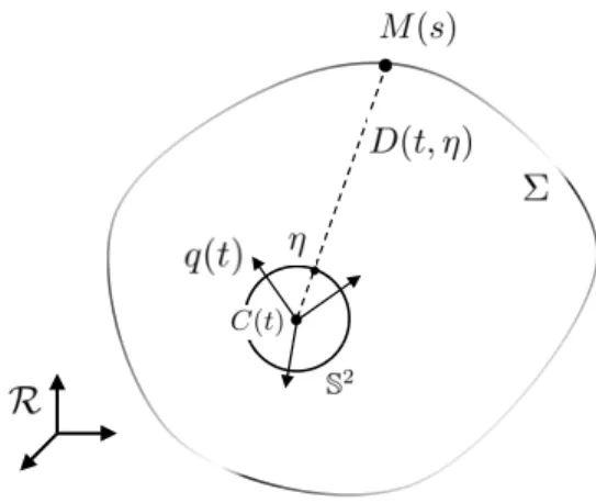
The generic model chosen in the following (PartsIandII) is a spherical model: the projection surface is a unit three dimensional sphere (S2
) and the projection center its center, denoted by C(t) as previously. The coordinates of C(t) are expressed in the reference frame RW. Orientation
of the camera is given by the quaternion q(t): any vector ς in the camera frame Rcamcorresponds
to the vector qςq∗ in the reference frame RW using the identification of vectors as imaginary
quaternions (see Appendix C.1.2). A pixel is labeled by the unit vector η in the camera frame: η belongs to the sphere S2 and receives the brightness y(t, η). Thus at each time t, the image produced by the camera is described by the scalar field S2
∋ η ↦ y(t, η) ∈ R. The notations of this model are represented in Figure 1.3. In this model, no particular axis is preferred to another, as it is the case in the pinhole model where the optical axis, orthogonal to the image plane partially defines orientation and direction of the camera reference frame.
1.3
Motion equations
1.3.1 Spherical model: the camera in a fixed environment
The motion of the camera is given through the linear and angular velocities v(t) and ω(t) expressed in the camera reference frame Rcam. Linear and angular velocities are related to the
time derivatives of position and orientation through the motion equations (see Appendix Cand
[Radix, 1980])
˙q=1
2qω and ˙C(t) = qvq
∗. (1.8)
The model adopted for the scene is based on two main assumptions:
– (H1): the scene is a closed, C1 and convex surface Σ of R3, diffeomorphic to S2;
– (H2): the scene is a Lambertian surface; – (H3): the scene is static.
Figure 1.3: Model and notations of a spherical camera in a static environment
[Bonnabel and Rouchon, 2009,Zarrouati et al., 2012c].
To be consistent with assumption (H1), the camera is inside the domain Ω⊂ R3
delimited by Σ= ∂Ω.
The first assumption implies that to a point M ∈ Σ corresponds one and only one camera pixel. At each time t, there is a bijection between the position of the pixel given by η∈ S2
and the point M ∈ Σ. Since the point M is labeled by s ∈ S2, this means that for each t, exist two
mappings S2
∋ s ↦ η = φ(t, s) ∈ S2
and S2
∋ η ↦ s = ψ(t, η) ∈ S2
with φ(t, ψ(t, η)) ≡ η and ψ(t, φ(t, s)) ≡ s, for all η, s ∈ S2. To summarize we have:
η= φ(t, s) and s = ψ(t, η) (1.9)
where ψ(t, .) and φ(t, .) are diffeomorphisms of S2
for every t > 0. Moreover, φ is implicitly defined by the relation
η= q(t)∗
ÐÐÐÐÐÐ→ C(t)M(s) ∥ÐÐÐÐÐÐ→C(t)M(s)∥
q(t) (1.10)
The density of light emitted by a point M(s) ∈ Σ does not depend on the direction of emission: this results from the second assumption (H2) on the scene. In addition, it is independent of t (H3). This means that y(t, η) depends only on s: there exists a function yΣ(s) such that
y(t, η) = yΣ(ψ(t, η)). (1.11)
In other words,
∂y
∂t∣s= 0. (1.12)
The distance ∥ÐÐÐÐÐÐ→C(t)M(s)∥ between the optical center and the object seen in the direction η = φ(t, s) is denoted by D(t, η).
D(t, η) ∶= ∥ÐÐÐÐÐÐÐÐÐÐ→C(t)M(ψ(t, η))∥. (1.13)
Let us consider the time derivative of the distance D attached to a specific point M(s): ∂D ∂t∣s= ∂∥ÐÐÐÐÐÐ→C(t)M(s)∥ ∂t RRRRRRRRRRRR s = ∂ÐÐÐÐÐÐ→C(t)M(s)∂t RRRRRRRRRR RRs ⋅ ÐÐÐÐÐÐ→C(t)M(s) ∥ÐÐÐÐÐÐ→C(t)M(s)∥ = −qvq∗⋅ qηq∗ using (1.8) and (1.10) = −v ⋅ η. (1.14)
The last relation holds since a dot product does not depend on the frame of reference in which it is computed. The meaning of equation (1.14) is simple: the distance between the camera and a specific point decreases as the camera moves towards that point.
On the other hand, the direction of observation η of a specific object M(s) in the camera frame evolves during the trajectory of the camera according to:
∂η ∂t∣s= ∂ ∂t ⎛ ⎝q∗ ÐÐÐÐÐÐ→ C(t)M(s) ∣∣C(t)M(s)∣∣q⎞⎠RRRRRRRRRRRRsusing (1.10) = q∗ ∂t∂ ⎛⎝∣∣C(t)M(s)∣∣ÐÐÐÐÐÐ→C(t)M(s) ⎞⎠RRRRRRRRRR RRs
q+ η × ω using (1.8) and properties of the quaternion product = q∗(q (−v D+ η v⋅ η D ) q ∗) q + η × ω using (1.8) = η × (ω + D1η× v). (1.15)
In a pure rotational motion (v= 0), this equation means that all objects move in the same way in the image: in other words, all pixels are relabeled with a different origin, which is consistent with the spherical geometry of the problem. If the trajectory of the camera is a translation (v ≠ 0), the objects move differently depending on their position with respect to the camera. Exactly as for a regular perspective camera, there is an intrinsic ambiguity in the projection of the trajectory of an object, due to the multiplicative term v
D: a monocular camera system can
not capture the scale factor of the perceived environment.
Tracking specific well-defined objects like we just did to obtain equations (1.12), (1.14) and (1.15), is somehow a Lagrangian approach. But these equations can be combined all together in a Eulerian approach, using chain rule differentiation: for any mapping S2
∈ η ↦ h(t, η) ∈ R, ∂h ∂t∣s= ∂h ∂t∣η+ ∂h ∂η∣t⋅ ∂η ∂t∣s . ∂h
∂η∣tis the gradient of h with respect to the Riemannian metric of S 2
(see SectionA.2), denoted ∇h in the following. Applied to the intensity y and the depth D, it yields
∂y ∂t∣η= −∇y ⋅ (η × (ω + 1 Dη× v)), (1.16) ∂D ∂t ∣η= −∇D ⋅ (η × (ω + 1 Dη× v)) − v ⋅ η, (1.17) where ∂y ∂t∣ηand ∂D
∂t∣ηstand for partial derivatives of y and D with respect to t: they are denoted
in the following ∂ty and ∂tD for sake of simplicity.
The first Partial Differential Equation (PDE) (1.16) is well-known in the literature, under a slightly different form, as the optical flow constraint (see [Horn and Schunck, 1981] and Part I for more details on optical flow). The second PDE (1.17) was introduced in
[Bonnabel and Rouchon, 2009]: the transport term is the same than in (1.16), but a second term
breaks the ambiguity of the scale factor. This very interesting property enables to solve many issues encountered in image processing: this will be the main topic of PartsIandII. By analogy with the optical flow constraint (1.16), this equation (1.17) is named in the following geometrical flow constraint. Equations (1.16) and (1.17) are SO(3)-invariant: they remain unchanged by any rotation described by the quaternion σ and changing (η, ω, v) to (σησ∗, σωσ∗, σvσ∗). 1.3.2 Pinhole-adapted model
To use this model with camera data, one needs to write the invariant equations (1.16) and (1.17) with local coordinates on S2
corresponding to a real camera model. We detail here the computations for a pinhole camera model, but as explained in Chapter 1, any single viewpoint model could be considered, as long as the mapping between a3Dpoint coordinates in the camera frame and its projection on the image plane is known. For the pinhole camera model, the pixel of coordinates(z1, z2) corresponds to the unit vector η ∈ S2 of coordinates in R3:
η=√ 1 1+ z2 1 + z 2 2 ⎛ ⎜ ⎝ z1 z2 1 ⎞ ⎟ ⎠.
The optical axis of the camera(z-axis in the notations introduced in Subsection1.1.1) corresponds here to the direction z3. Directions 1 and 2 correspond respectively to the horizontal axis from
left to right and to the vertical axis from top to bottom on the image frame (x-axis and y-axis respectively).
The gradients ∇y and ∇Γ must be expressed with respect to z1 and z2. Let us detail this
derivation for y. We use two properties of the Riemannian gradient: – ∇y is tangent to S2
, thus∇y ⋅ η = 0;
– the differential dy corresponds on one hand to ∇y ⋅ dη and on the other hand to ∂y ∂z1dz1+
∂y ∂z2dz2.
The computation of dη yields
dη= 1 (1 + z2 1+ z 2 2) 3/2 ⎛ ⎜ ⎝ 1+ z2 2 −z1z2 −z1 ⎞ ⎟ ⎠dz1+ 1 (1 + z2 1+ z 2 2) 3/2 ⎛ ⎜ ⎝ −z1z2 1+ z12 −z2 ⎞ ⎟ ⎠dz2. (1.18) 18
Then, by identification of∇y with a vector of R3
expressed in the camera frame, one writes ∇y =⎛⎜ ⎝ ∇y1 ∇y2 ∇y3 ⎞ ⎟ ⎠. This yields for dy
∇y ⋅ dη =(1 + z21 1+ z 2 2) 3/2[(∇y1(1 + z 2 2) − ∇y2(z1z2) − ∇y3(z1))dz1 + (−∇y1(z1z2) + ∇y2(1 + z 2 1) − ∇y3(z2))dz2]. (1.19)
Then,∇y ⋅ η = 0 yields
∇y3= −∇y1z1− ∇y2z2. (1.20)
Equation (1.20) is plugged in (1.19), then by identification of dy with ∂y ∂z1dz1+ ∂y ∂z2dz2, one gets: ∇y =√1+ z2 1+ z 2 2 ⎛ ⎜⎜ ⎝ ∂y ∂z1 ∂y ∂z2 −z1∂z∂y 1 − z2 ∂y ∂z2 ⎞ ⎟⎟ ⎠ . (1.21)
Similarly we get the three coordinates of∇Γ. Injecting these expressions in (1.16) and (1.17) yields the followingPDEscorresponding to (1.16) and (1.17) in local pinhole coordinates:
∂ty= − ∂y ∂z1(z 1z2ω1− (1 + z1 2 )ω2+ z2ω3+ 1 D √ 1+ z2 1+ z 2 2(−v1+ z1v3)) −∂z∂y 2((1 + z 22)ω1− z1z2ω2− z1ω3+ 1 D √ 1+ z2 1+ z 2 2(−v2+ z2v3)) (1.22) ∂tD= − ∂D ∂z1 (z 1z2ω1− (1 + z1 2 )ω2+ z2ω3+ 1 D √ 1+ z2 1+ z 2 2(−v1+ z1v3)) −∂D∂z 2((1 + z 22)ω1− z1z2ω2− z1ω3+ 1 D √ 1+ z2 1+ z 2 2(−v2+ z2v3)) − (z1v1+ z2v2+ v3) (1.23)
where v1, v2, v3, ω1, ω2, ω3 are the components of linear and angular velocities in the camera
Chapter 2
Formulation as a minimization problem
La profondeur, solution d’un problème inverse
Dans ce chapitre sont décrites les méthodes variationnelles et leurs applications à l’estimation du flot optique. Les plus connues de ces techniques d’estimation, la méthode d’Horn-Schunck et la méthode TV-L1, sont détaillées. De telles méthodes peuvent être adaptées à l’estimation de profondeur par la minimisation de notre contrainte de flot optique spécifique (1.16) plutôt que de la contrainte de flot optique classique : le mouvement apparaissant explicitement, le problème est bien posé au sens où, à chaque pixel de l’image, une équation scalaire est associée à l’unique inconnue du problème, la profondeur. Ces méthodes ont été présentées dans
[Zarrouati et al., 2012a,Zarrouati et al., 2012b,Zarrouati et al., 2012c].
In this chapter, variational methods and their application to optical flow estimation are described. The most well-known, the Horn and Schunck and the TV-L1 optical flow estimation
methods are detailed. Such methods can be adapted to depth estimation by the minimization of our invariant optical flow constraint (1.16) where motion is made explicit, instead of the regular optical flow constraint: the problem is well-posed and geometrically constrained in the sense that at each pixel, one scalar equation is associated to the only unknown of the problem, the depth. These methods were presented in [Zarrouati et al., 2012a, Zarrouati et al., 2012b,
Zarrouati et al., 2012c].
2.1
Variational methods applied to optical flow estimation
2.1.1 Optical flow
In [Horn and Schunck, 1981], Horn and Schunck described a method to compute the optical
flow, defined as "the distribution of apparent velocities of movement of brightness patterns in an image". The entire method is based on the assumption that the light intensity emitted by a specific object does not depend on time or direction of observation (assumptions (H2) and (H3) of the Section1.3.1 and the consequent equation (1.12)). Provided that the same physical point
is observed in two different images y1 and y2, the following equality holds:
y1(z1, z2) = y2(z1+ δz1, z2+ δz2)
where z ∶= (z1, z2) is the position of the point in the first image, and (δz1, δz2) is the apparent
displacement of the point between the two images. If the images are only separated by a short time interval δt, it is natural to introduce an apparent velocity vector (V1, V2) ∶= δt1(δz1, δz2).
Extending this apparent velocity concept to the whole image yields a velocity field V(t, z) ∶= (V1, V2)(t, z1, z2) named optical flow. First order differentiation in both time and space yields
the so-called optical flow constraint: ∂y ∂t + V1 ∂y ∂z1 + V 2 ∂y ∂z2 = 0. (2.1) This equation can be identified with equation (1.22): an explicit expression of V1 and V2 with
respect to velocity and depth is given in the following (see equations (2.10) and (2.11)). 2.1.2 Variational methods applied to inverse problems
An important field of image processing is devoted to image restoration: the object is to improve the quality of a given damaged image. The term "damage" covers a wide range of effects, from additional noise to missing pixel data or blur. The usual formulation of restoration is the following: one aims to reconstruct the ideal input y0 given an output y (the image) related
by
y= Ky0+ ν
where ν designates noise and K is a linear operator that describes the "damaging" effect. For example, to restore
– a noisy image: K is simply the identity (noise is already taken into account in ν); – a blurred image: K is the convolution with a Gaussian kernel;
– an image where pixel data are missing: K is the characteristic function 1S of a discrete set
S.
Variational methods (specifically variational minimization) apply to inverse problems as the solution is claimed to be the argument of the following minimized functional
∫ ∣∣y − Ky0∣∣ + α 2
J(y) where
– J is a prior, in other words a weighting function of the image,
– ∫ ∣∣y − Ky0∣∣ is the data fidelity term, usually the sum over the whole rectangular frame
occupied by the image of the residuals, and – α2
is a strictly positive parameter allowing to scale the influence of the prior term in the minimization task.
Many priors have been proposed in the recent years, and generally each one is very well adapted to a specific class of images. The most well known are the Sobolev prior and the total variation prior. The data fidelity term usually takes into play the Euclidean norm (L2) but can be in some cases
more sophisticated. For more details on variational minimization applied to inverse problems and the links between variational methods and PDEs methods, see [Peyré, 2013], [Grasmair, 2010],
or [Guichard and Morel, 2004]. Variational methods have also been applied to other estimation
problems, and in particular to optical flow estimation, for which two formulations are detailed in the following.
2.1.3 Variational method with Sobolev prior
For optical flow estimation, Horn and Schunck proposed the data fidelity term to be replaced by the optical flow constraint (2.1) in L2
norm. The prior used for J is the Sobolev prior, defined as the L2
norm of the gradient, applied to optical flow: J(V1, V2) = ∣∣∇V1∣∣
2
L2+ ∣∣∇V2∣∣ 2 L2.
This yields that the apparent velocity field V = (V1, V2) is estimated for each time t by minimizing
versus W ∶= (W1, W2) the following cost (the image I is the rectangle of R2 occupied by the
image) I(W) = ∬ I(( ∂y ∂t + W1 ∂y ∂z1 + W 2 ∂y ∂z2) 2 + α2 (∇W1 2 + ∇W2 2 ))dz1dz2 (2.2)
where∇ is the gradient operator in the Euclidean plane (z1, z2) and the partial derivatives ∂y∂t, ∂y
∂z1 and
∂y
∂z2 are assumed to be known. The Sobolev prior is a regularizing term, and α> 0 is a
regularization parameter: when used for image restoration, it yields to a formulation where the solution of the minimization problem is the solution of the heat equation and can be explicitly deduced from the image y by convolution with a Gaussian kernel.
Notice that for optical flow estimation, the prior term is necessary to solve a fundamentally ill-posed problem where for each position in an image, two components of a vector are estimated from only one scalar equation. Here, the Sobolev prior comes from the assumption that the velocity field is only submitted to small spatial variations: this is a reasonable assumption in an environment where the depth D is continuous, regular and lower-bounded as shown by the following identification ((2.10) and (2.11)).
Such Horn-Schunk estimation of V at time t is denoted by VHS(t, z) ∶= (VHS1(t, z), VHS2(t, z)).
For each time t, minimization of the cost I is computed using usual calculus of variation, as the velocity field solution VHS satisfies the system of Euler-Lagrange equations obtained as first-order
stationary equations for I: ∂y ∂z1 ∂y ∂t + ( ∂y ∂z1) 2 VHS1+ ∂y ∂z1 ∂y ∂z2 VHS2− α 2 ∆VHS1 = 0 ∂y ∂z2 ∂y ∂t + ∂y ∂z1 ∂y ∂z2 VHS1+ ( ∂y ∂z2) 2 VHS2− α 2 ∆VHS2 = 0
with boundary conditions ∂VHS 1
∂n =
∂VHS 2
∂n = 0 (n the normal to ∂I). Here ∆ is the Laplacian
operator in the Euclidean space(z1, z2). The numerical resolution is usually based on
1. Computations of ∂y ∂z1,
∂y
∂z2 and
∂y
∂t via differentiation filters (e.g. Sobel filtering)
directly from the image data at different times around t. For example, ∂y
∂z1 can be
approximated using a central finite difference scheme (among others) by ∂y
∂z1(z
1, z2, t) ≈
y(z1+ δ, z2, t) − y(z1− δ, z2, t)
2δ ∶= Dyz1(z1, z2, t). (2.3)
To minimize the impact of noise on this differentiation scheme, a slight smoothing of the resulting derivative along the orthogonal direction (z2 in this example) is required. Using
the above definition (2.3) yields ∂y
∂z1(z
1, z2, t) ≈
1
4(2Dyz1(z1, z2, t) + Dyz1(z1, z2− δ, t) + Dyz1(z1, z2− δ, t)) . (2.4)
When δ is the length of the square pixels of the grid where image data are available, (2.4) can be expressed as a convolution operator: an approximation of ∂y
∂z1(z1, z2, t) is obtained
by convolution of y with the following kernel: 1 8δ ⎛ ⎜ ⎝ 1, 0, −1 2, 0, −2 1, 0, −1 ⎞ ⎟ ⎠.
2. Approximation of ∆VHS1 and ∆VHS2 by the difference between the weighted
mean of VHS1 and VHS2 on the neighboring pixels and their values at the current
pixel. The most common approximation of the discrete Laplacian ∆Df of a function
f(z1, z2) is given by
∆Df ≈
f(z1− δ, z2) + f(z1+ δ, z2) + f(z1, z2− δ) + f(z1, z2+ δ) − 4f(z1, z2)
δ2
in the case where f is known at every vertex of a square grid with length spacing δ. Thus, a fast computation of ∆Df is
¯ fn−nf
δ2 (here n= 4) where ¯fn is computed as the convolution
of f with Kn, here K4= ⎛ ⎜ ⎝ 0, 1, 0 1, 0, 1 0, 1, 0 ⎞ ⎟ ⎠.
This yields the following system of linear equations in (VHS1, VHS2) at each pixel of the
image: ⎧⎪⎪⎪⎪ ⎨⎪⎪⎪ ⎪⎩ ((∂y ∂z1) 2 + nα2 δ2) VHS1+ (∂z∂y 1 ∂y ∂z2) VHS2= α2 δ2(Kn∗ VHS1) − ∂z∂y 1 ∂y ∂t (∂y ∂z1 ∂y ∂z2) VHS1+ (( ∂y ∂z2) 2 + nα2 δ2) VHS2= α 2 δ2(Kn∗ VHS2) − ∂z∂y 2 ∂y ∂t. (2.5) 24
3. Iterative resolution (Jacobi scheme) of the linear system (2.5) in VHS1 and VHS2.
Defining VHS1 = 1
nKn∗ VHS1 and VHS2 = 1
nKn∗ VHS2, the inversion of (2.5) at each pixel
writes ⎧⎪⎪⎪⎪ ⎨⎪⎪⎪ ⎪⎩ ((∂y ∂z1) 2 + (∂y ∂z2) 2 + nα2 δ2) VHS1 = (nα 2 δ2 + ( ∂y ∂z2) 2 ) VHS1− (∂z∂y 1 ∂y ∂z2) VHS2− ∂y ∂z1 ∂y ∂t ((∂y ∂z1) 2 + (∂y ∂z2) 2 + nα2 δ2) VHS2 = (nα 2 δ2 + ( ∂y ∂z1) 2 ) VHS2− (∂z∂y 1 ∂y ∂z2) VHS1− ∂y ∂z2 ∂y ∂t. (2.6)
However, as VHS1 and VHS2 implicitly depend on VHS1 and VHS2, the closed form solution
of the problem (2.6) would require to invert a system of equations whose length is twice the size of an image, which is computationally not optimal. Alternatively, an iterative computation of the solution of this system appears, rewriting (2.6) as
⎧⎪⎪⎪⎪ ⎪⎪⎪⎪ ⎨⎪⎪⎪ ⎪⎪⎪⎪⎪ ⎩ VHS1 = VHS1− (∂y ∂z1) 2
VHS 1+(∂z1∂y ∂z2∂y)VHS 2+∂z1∂y ∂y∂t
((∂y ∂z1) 2 +(∂y ∂z2) 2 +nα2 δ2) = V1(VHS1, VHS2, y) VHS2 = VHS2− (∂y ∂z2) 2
VHS 2+(∂z1∂y ∂z2∂y)VHS 1+∂z2∂y ∂y∂t
((∂y ∂z1) 2 +(∂y ∂z2) 2 +nα2 δ2) = V2(VHS1, VHS2, y) . (2.7)
This form shows that VHS1 and VHS2 can be iteratively computed, applying the operators
V1 and V2 to the result of the previous iteration.
The convergence of this numerical method of resolution
was proven in [Mitiche and reza Mansouri, 2004]. Three parameters have a direct impact on the speed of convergence and on the precision: the regularization parameter α, the number of iterations for the Jacobi scheme and the initial values of VHS1 and VHS2 at the beginning of this
iteration step. To be specific, α should neither be too small in order to filter noise appearing in differentiation filters applied on y, nor too large in order to have VHS close to V when∇V ≠ 0.
2.1.4 Variational method with total variation prior
In their seminal article [Rudin et al., 1992], Rudin, Osher and Fatemi proposed for image denoising the total variation prior defined by the sum of the gradients in L1 norm. Its main
advantage resides in the fact that edges are better conserved: the smoothing/regularizing effect related to diffusion in the heat equation is attenuated. This prior enables the extension of variational methods to non-smooth functions, and is well-adapted to piecewise constant images (cartoon images). It can however sometimes lead to a staircase effect. The main issue with total variation prior comes from the non differentiability of this prior at point 0. A solution to this problem consists in the following approximation:
∫ ∣∣∇f∣∣ ≈ ∫ √ǫ2+ ∣∣∇f∣∣2
where ǫ is a small positive constant, which is differentiable. Another solution is based on dual formulation of the minimization task and was introduced by Chambolle in [Chambolle, 2004]
along with a convergent iterative scheme summarized in the following. The solution of the minimization task min y ∫ ∣∣∇y∣∣ + β 2 ∣∣y − yd∣∣ 2 is given by y= yd+ 1 2β2∇ ⋅ p (2.8)
where p= (p1, p2) is the dual variable and ∇ ⋅ p denotes the Euclidean divergence of the vector
field p. The dual variable is computed iteratively by ˜ pn= pn−1+ 2β2τ(∇(yd+ 1 2β2∇ ⋅ pn−1)) and then pn= ˜ pn max(1, ∣˜pn∣)
where p0 = 0 and the time step τ ≤ 1/4.
When, in addition, the data fidelity term∣∣y−yd∣∣ also involves L1norm, the method is known
as TV-L1
minimization, and a solution consists of dividing the problem in two minimization sub-tasks. An auxiliary variable ya is introduced, and the functional to minimize is approximated
by
Fβ = ∫ ∣∣∇y∣∣ + α2∣∣ya− yd∣∣ + β2∣∣y − ya∣∣2
where β is a small positive constant. Then, the minimization process of Fβconsists of alternating
1. min y ∫ ∣∣∇y∣∣ + β 2 ∣∣y − ya∣∣ 2
for which a solution is given by (2.8), and 2.
min
ya ∫ α
2
∣∣ρ(ya)∣∣ + β2∣∣y − ya∣∣2
where ρ(ya) designates the residuals associated to the auxiliary variable ya. The second step can
be solved point-wise if the residual ρ(ya) does not depend on spatial derivatives of ya.
This method was applied to optical flow estimation in [Chambolle and Pock, 2010] and
[Wedel et al., 2009]. In that case, the residual ρ(y) is simply the optical flow constraint,
which is linear with respect to the optical flow components. This yields that the second step optimization is performed using regular optimization methods (e.g. Karush-Kuhn-Tucker conditions) combined with thresholding steps (see [Wedel et al., 2008]):
ya= y + ⎧⎪⎪⎪⎪ ⎪⎨ ⎪⎪⎪⎪⎪ ⎩ α2 2β2∇y if ρ(y) < − α2 2β2∣∣∇y∣∣ 2 −α2 2β2∇y if ρ(y) > α2 2β2∣∣∇y∣∣ 2
−ρ(y)∣∣∇y∣∣∇y2 if ∣ρ(y)∣ ≤
α2
2β2∣∣∇y∣∣
2
. (2.9)
2.2
Variational methods applied to depth estimation
We described in Chapter1.3a slightly different form of optical flow constraint, where linear and angular velocities appear explicitly and optical flow as a vector field is implicit. Expressing (1.16) in pinhole coordinates (see (1.22)) yields a precise identification of optical flow components with respect to velocities v and ω and depth D:
V1(t, z) = f1(z, ω(t)) + 1 D(t, z)g1(z, v(t)) V2(t, z) = f2(z, ω(t)) + 1 D(t, z)g2(z, v(t)) (2.10) with f1(z, ω) ∶= z1z2ω1− (1 + z12)ω2+ z2ω3 g1(z, v) ∶= √ 1+ z2 1+ z 2 2(−v1+ z1v3) f2(z, ω) ∶= (1 + z22)ω1− z1z2ω2− z1ω3 g2(z, v) ∶= √ 1+ z2 1+ z 2 2(−v2+ z2v3) (2.11)
where ω= (ω1, ω2, ω3)T and v = (v1, v2, v3)T are expressed in the camera reference frame Rcam
(see Section1.3.2 for notations). Assuming that linear and angular velocities are known inputs, the structure of optical flow is well determined: in addition, it is linear with respect to Γ∶= 1/D the inverse of depth. We will describe in the following how one can take advantage of this linear dependence and the knowledge of motion to adapt usual variational methods of optical flow estimation to depth estimation. Let us highlight the fact that depth only appears in the expressions (2.10) multiplied by the terms g1and g2which directly depend on the linear velocity:
in others words, linear motion is necessary to estimate depth. In addition, the quality of depth estimation directly depends on the magnitude of linear velocity. This a well-known effect in stereo-vision where the choice of the baseline between the cameras is the result of a trade off between performance and practical considerations.
2.2.1 Estimation of depth with Sobolev priors
Instead of minimizing the cost I given by (2.2) with respect to the optical flow components W1 and W2, let us define a new invariant cost JHS associated to our optical flow constraint
(1.16), JHS(Υ) = ∬ I( ( ∂y ∂t + ∇y ⋅ (η × (ω + Υη × v))) 2 + α2 ∇Υ2 )dση (2.12)
and minimize it with respect to any inverse depth profileI ∋ η ↦ Υ(t, η) ∈ R. The time t is fixed here and dση is the Riemannian infinitesimal surface element on S2. I ⊂ S2 is the domain where
The first order stationary condition of JHS with respect to any variation of Υ yields the
following invariant PDEcharacterizing the resulting estimation ΓHS of Γ in pinhole cordinates:
α2∆ΓHS= (
∂y
∂t + ∇y ⋅ (η × (ω + ΓHSη× v))) (∇y ⋅ (η × (η × v))) on I (2.13) ∂ΓHS
∂n = 0 on ∂I (2.14)
where ∆ΓHS is the Laplacian of ΓHS on the Riemannian sphere S
2
and ∂I is the boundary of I, assumed to be piece-wise smooth and with unit normal vector n.
In pinhole coordinates, recall from Section 1.3.2 that dση = (1 + z12+ z 2 2) −3/2 dz1dz2 ∇Υ2 = (1 + z2 1+ z 2 2) ( ∂Υ ∂z1 2 +∂z∂Υ 2 2 + (z1 ∂Υ ∂z1 + z 2 ∂Υ ∂z2) 2 ) (∂y∂t + ∇y ⋅ (η × (ω + Υη × v)))2= (F + ΥG)2 where F ∶=∂y ∂t + f1(z, ω) ∂y ∂z1 + f 2(z, ω) ∂y ∂z2 G∶= g1(z, v) ∂y ∂z1 + g 2(z, v) ∂y ∂z2 . (2.15)
Consequently, the first order stationary condition (2.13) reads in(z1, z2) coordinates:
ΓHSG 2 + FG = α2 (1 + z2 1+ z 2 2) 3/2⎡⎢ ⎢⎢ ⎢⎣ ∂ z1 ⎛ ⎝ 1+ z2 1 √ 1+ z2 1+ z 2 2 ∂ΓHS ∂z1 ⎞ ⎠ +z∂ 2 ⎛ ⎝ 1+ z2 2 √ 1+ z2 1+ z 2 2 ∂ΓHS ∂z2 ⎞ ⎠ +z∂ 2 ⎛ ⎝ z1z2 √ 1+ z2 1+ z 2 2 ∂ΓHS ∂z1 ⎞ ⎠ +z∂ 1 ⎛ ⎝ z1z2 √ 1+ z2 1+ z 2 2 ∂ΓHS ∂z2 ⎞ ⎠ ⎤⎥ ⎥⎥ ⎥⎦ (2.16)
on the rectangular domainI ∶= [−¯z1, ¯z1] × [−¯z2, ¯z2] (¯z1, ¯z2> 0 with ¯z21+ ¯z 2 2 < 1).
The right term of (2.16) corresponds to the Laplacian operator on the Riemannian sphere S2
multiplied by α2 in pinhole coordinates by identification with (2.13). At the center of the image,
it is equivalent to the Euclidean Laplacian, but as the direction of observation η moves towards the corners of the rectangular matrix of pixels, (the absolute value of pixel coordinates z1 and
z2 increase), the correction due to the reprojection of the equation on S2 back to a regular plane
can not be neglected. As a numerical example, let us consider that the visible portion of the environment is a plane, orthogonal to the optical axis. The equation describing this plane is
Γ(z1, z2) = Γ0 √ 1+ z2 1+ z 2 2 .
The Euclidean Laplacian ∆EΓ and the Riemannian Laplacian ∆RΓ of this function write
respectively ∆EΓ(z1, z2) = Γ0(z21+ z 2 2− 2) (1 + z2 1+ z 2 2) 5/2, ∆RΓ(z1, z2) = − 2Γ0 √ 1+ z2 1+ z 2 2 .
Notice that the Riemannian Laplacian ∆RΓ can be computed by two different methods: first,
using the identification of the Laplacian with the right term of the expression (2.16); secondly, using the differential calculus expression (A.4) applied to Γ(η) = Γ0η⋅ (0, 0, 1)T.
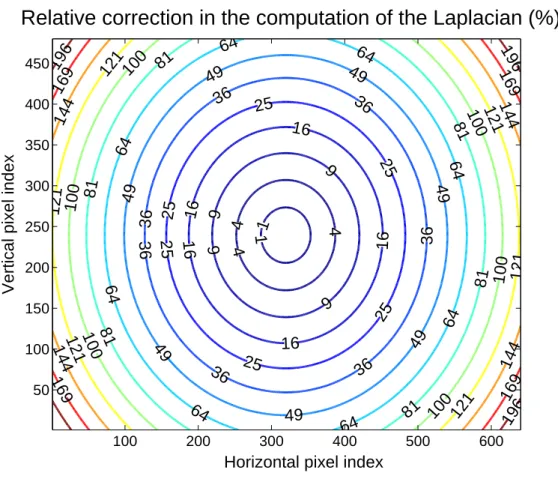
Figure2.1graphically represents the relative difference ∣∆EΓ−∆RΓ∣
∣∆EΓ∣ over the whole image: the
relative error reaches 200% in the corners in the image, for a camera with a total field of view of 60° by 50° (horizontally and vertically, respectively).
The numerical resolution of this scalar diffusion equation providing the estimation ΓHS of Γ
is similar to the one used for the Horn-Schunck estimation VHS of V , except for the evaluation
of the Laplacian, which is adapted to the spherical model.
2.2.2 Estimation of depth by total variation minimization
For total variation minimization as in subsection 2.1.4, both our optical flow constraint and the regularization term are taken into account in L1
norm in the functional JT V−L1 to minimize:
JT V−L1(Γ) = ∫
I(α
2
∣∣∂y
∂t+ ∇y ⋅ (η × (ω + Γη × v))∣∣ + ∣∣∇Γ∣∣) dση (2.17) where dση is the Riemannian infinitesimal surface element on S2 and α is a parameter that
weights between the data fidelity and the regularization terms. As described for optical flow estimation, the minimization strategy used is divided in two tasks:
1. For Λ being fixed, find the argument Γ of the minimum of J1(Γ) = ∫
I(∣∣∇Γ∣∣ + β 2
(Γ − Λ)2
) dση (2.18)
2. For Γ being fixed, find the argument Λ of the minimum of J2(Λ) = ∫ I(α 2 ∣∣ρ(Λ)∣∣ + β2 (Γ − Λ)2 ) dση (2.19) where ρ(Λ) = ∂y
∂t + ∇y ⋅ (η × (ω + Λη × v)) is the depth residual.
The main algorithm steps are given by the following: – Initialization: Γ0
= 0, Λ0
= 0, ¯Γ0
= 0 p0