Local Linear Convergence of Douglas–Rachford/ADMM
for Low Complexity Regularization
Jingwei Liang∗, Jalal M. Fadili∗, Gabriel Peyr´e†and Russell Luke‡
∗GREYC, CNRS, ENSICAEN, Universit´e de Caen, Email:{Jingwei.Liang, Jalal.Fadili}@ensicaen.fr †CNRS, Ceremade, Universit´e Paris-Dauphine, Email: [email protected]
‡Institut f¨ur Numerische und Angewandte Mathematik, Universit¨at G¨ottingen, Email: [email protected]
Abstract—The Douglas–Rachford (DR) and ADMM algorithms have become popular to solve sparse recovery problems and beyond. The goal of this work is to understand the local convergence behaviour of DR/ADMM which have been observed in practice to exhibit local linear convergence. We show that when the involved functions (resp. their Legendre-Fenchel conjugates) are partly smooth, the DR (resp. ADMM) method identifies their associated active manifolds in finite time. Moreover, when these functions are partly polyhedral, we prove that DR (resp. ADMM) is locally linearly convergent with a rate in terms of the cosine of the Friedrichs angle between the tangent spaces of the two active manifolds. This is illustrated by several concrete examples and supported by numerical experiments.
I. INTRODUCTION In this work, we consider the problem of solving
min
x∈RnJ(x) + G(x), (1)
where both J and G are in Γ0(Rn), the class of proper, lower
semi-continuous and convex functions. We assume thatri(domJ) ∩ ri(domG) 6= ∅, where ri(C) is the relative interior of the nonempty convex set C, and domF is the domain of the function F . We also assume that the set of minimizers of (1) is non-empty, and the two functions are simple (proxγJ,proxγG, γ > 0, are easy to compute), where the proximity operator is defined, for γ > 0, as proxγJ(z) = argminx∈Rn
1 2||x − z||
2
+ γJ(x).
An efficient and provably convergent algorithm for solving (1) is the DR method [1], which reads, in its relaxed form,
( zk+1= (1 − λk)zk+ λkBDRz k , xk+1= proxγJz k+1 , (2) where BDR def. = 1
2`(2proxγJ− Id) ◦ (2proxγG− Id) + Id´, for γ >
0, λk∈]0, 2] withPk∈Nλk(2 − λk) = +∞.
Since the set of minimizers of (1) is non-empty, so is the set of fixed pointsfix(BDR) since the former is nothing but proxγJ(fix(BDR)).
See [2] for a more detailed account on DR. Though we focus in the following on DR, all our results readily apply to ADMM since it is the DR applied to the Fenchel dual problem of (1).
II. PARTLYSMOOTHFUNCTIONS ANDFINITEIDENTIFICATION Beside J, G∈ Γ0(Rn), our central assumption is that J, G are
partly smooth functions. Partial smoothness was originally defined in [3]. Here we specialize it to the case of functions inΓ0(Rn). Denote
par(C) the subspace parallel to the non-empty convex set C ⊂ Rn.
Definition II.1. Let J∈ Γ0(Rn) and x ∈ Rnsuch that ∂J(x) 6= ∅.
J is partly smooth at x relative to a setM containing x if (Smoothness) M is a C2
-manifold, J|Mis C2 around x;
(Sharpness) The tangent spaceTx(M) = Tx
def.
= par(∂J(x)); (Continuity) The ∂J is continuous at x relative toM. The class of partly smooth functions at x relative to M is denoted asPSFx(M).
The class of PSF is very large. Popular examples in signal processing and machine learning include ℓ1, ℓ1,2, ℓ∞ norms, TV
semi-norm and nuclear norm, see also [4].
Now define the variable vk= proxγG(2proxγJ− Id)z k
. Theorem II.2 (Finite activity identification). Let the DR scheme (2) be used to create a sequence(zk, xk, vk). Then (zk, xk, vk) →
(z⋆
, x⋆, x⋆), where z⋆
∈ fix(BDR) and x⋆is a global minimizer of
(1). Assume that J∈ PSFx⋆(MJ
x⋆), G ∈ PSFx⋆(MG
x⋆), and
z⋆∈ x⋆+ γ`ri(∂J(x⋆
)) ∩ ri(−∂G(x⋆))´. (3)
Then, the DR scheme has the finite activity identification property, i.e. for allk sufficiently large,(xk, vk) ∈ MJ
x⋆× MGx⋆.
Condition (3) implies that0 ∈ ri(∂J(x⋆) + ∂G(x⋆)), which can be
viewed as a geometric generalization of the strict complementarity of non-linear programming. In a compressed sensing scenario, it can be guaranteed for a sufficiently large number of measurements.
III. LOCALLINEARCONVERGENCE OFDR
We now turn to local linear convergence properties of DR for the case of locally polyhedral functions. This is a subclass of partly smooth functions, whose epigraphs look locally like a polyhedron. In the following, we will refer to the Friedrichs angle between two subspaces V and W , denoted θF(V, W ). In fact, θF(V, W )
is the (d + 1)-th principal angle between V and W , where d = dim(V ∩ W ), see also [5].
Theorem III.1. Assume thatJ and G are locally polyhedral, and the conditions of Theorem II.2 hold withλk≡ λ. Then there exists
K >0 such that for all k > K,
||zk− z⋆|| 6 ρk||z0− z ⋆ ||, (4) whereρ=p(1 − λ)2+ λ(2 − λ) cos2θ F(TxJ⋆, T G x⋆) ∈ [0, 1[.
This rate is optimal. For the special case of basis pursuit, we recover the result of [6], but with less stringent assumptions.
IV. NUMERICALEXPERIMENTS
As examples, we consider the ℓ1, ℓ∞ norms and the anisotropic
TV semi-norm which are all polyhedral, hence partly smooth relative the following subspaces
ℓ1: Tx= {u ∈ Rn: supp(u) ⊆ supp(x)},
ℓ∞: Tx=˘u : uI = rsI, r∈ R¯, s = sign(x), I = {i : |xi| = ||x||∞},
TV: Tx=˘u ∈ Rn: supp(∇u) ⊆ I¯, I = supp(∇x),
where∇ is the gradient operator.
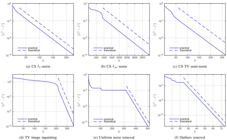
Figure1 displays the observed and predicted convergence profiles of DR when solving several problem instances, including compressed sensing, denoising and inpainting.
k 50 100 150 200 k z k! z ?k 10-10 10-6 10-2 102 practical theoretical (a) CS ℓ1-norm k 500 1000 1500 2000 2500 3000 3500 k z k! z ?k 10-10 10-6 10-2 102 practical theoretical (b) CS ℓ∞-norm k 50 100 150 200 250 k z k! z ?k 10-10 10-6 10-2 102 practical theoretical (c) CS TV semi-norm k 50 100 150 200 250 k z k! z ?k 10-10 10-6 10-2 102 practical theoretical (d) TV image inpainting k 100 200 300 400 500 k z k! z ?k 10-10 10-6 10-2 102 practical theoretical
(e) Uniform noise removal
k 10 20 30 40 50 60 70 k z k! z ?k 10-10 10-6 10-2 practical theoretical (f) Outliers removal
Fig. 1. Observed (solid) and predicted (dashed) convergence profiles of DR (2) in terms of||zk− z⋆||. For the first 4 subfigures, we solve a problem of the
formminx∈RnJ(x) s.t. Ax = y, where A is either drawn randomly from the standard Gaussian ensemble (CS), or random binary (inpainting). (a) CS with
J= || · ||1, A∈ R48×128. (b) CS with J= || · ||∞, A∈ R120×128. (c) CS with J= || · ||TV, A∈ R48×128. (d) TV image inpainting, A∈ R512×1024.
(e) Uniform noise removal by solvingminx∈R128||x||TVs.t. ||x − y||∞6δ. (f) Outliers removal by solvingminx∈R128λ||x||TV+ ||x − y||1. The starting
points of the dashed lines are the iteration at which the active subspaces are identified.
ACKNOWLEDGMENT
This work has been partly supported by the European Research Council (ERC project SIGMA-Vision). JF was partly supported by Institut Universitaire de France.
REFERENCES
[1] P. L. Lions and B. Mercier, Splitting algorithms for the sum of two nonlinear operators, SIAM Journal on Numerical Analysis, 16(6):964– 979, 1979.
[2] H. H. Bauschke and P. L. Combettes, Convex analysis and monotone operator theory in Hilbert spaces, Springer, 2011.
[3] A. S. Lewis, Active sets, nonsmoothness, and sensitivity, SIAM Journal on Optimization, 13(3):702–725, 2003.
[4] S. Vaiter, G. Peyr´e, and M. J. Fadili, Partly smooth regularization of inverse problems, arXiv:1405.1004, 2014.
[5] H. H. Bauschke, J.Y. Bello Cruz, T.A. Nghia, H. M. Phan, and X. Wang, Optimal rates of convergence of matrices with applications, arxiv:1407.0671, 2014.
[6] L. Demanet and X. Zhang, Eventual linear convergence of the Douglas– Rachford iteration for basis pursuit, Mathematical Programming, 2013.