Inside the Black Box: Why are Order Flows Models of Exchange Rate more competitive than Traditional Models of Exchange Rate?

Inside the Black Box: Why are Order Flows Models of Exchange Rate more competitive than Traditional Models of Exchange Rate?

Gabriele Di Filippo1

Department of Economics, LEDA-SDFi, University Paris Dauphine

Preliminary Version: October 2009 Revised Version: January 2011

Abstract

This article looks inside the black box of order flows to understand why order flows models of exchange rate are more competitive than traditional models of exchange rate. We set a theoretical model that relies on a behavioural exchange rate model and a microstructure model. The model puts forward three results. First, simulations replicate stylised facts observed in the foreign exchange market. Secondly, the model shows that the foreign exchange market is intrinsically inefficient. Incoming information is distorted by behavioural noise and microstructure noise. Thirdly, order flows models of exchange rate provide an answer to the exchange rate disconnection puzzle. Indeed, order flows contain processed information i.e. a time-varying weight of fundamental information, behavioural information and microstructure information while traditional models only consider raw information i.e. fundamental information.

Keywords: Behavioural Finance, Microstructure, Order Flows Models, Market Efficiency,

Exchange Rate Disconnection Puzzle

JEL Codes: F31, G1, G15

1

Author Contact: gabriele.di_filippo@yahoo.fr; University Paris IX Dauphine, Office B313, Place du Maréchal de Lattre de Tassigny 75775 Paris CEDEX 16, France ; Acknowledgements: I am grateful to helpful comments from the participants of the PhD seminars in financial macroeconomics organised by the doctoral school of the University Paris IX Dauphine and to participants at the workshop “Market Microstructure: confronting many viewpoints” organised by the Institut Louis Bachelier. I am very grateful to two anonymous referees at the journal Finance. All the remaining errors are of the author only.

1. Introduction

Following decades of empirical failure to explain and forecast exchange rates

dynamics based on traditional exchange rate models (Meese and Rogoff, (1983), Cheung et

al. (2005)), the recent microstructure literature offers promising results. Microstructure

models based on order flows provide better explanatory and predictive powers in forecasting exchange rate dynamics than traditional models; especially at short horizons (Evans and Lyons (2002a, 2002b), Danielsson et al. (2002), Berger et al. (2008), Chinn and Moore (2008)). To justify this performance, order flows theorists claim that order flow includes private information about exchange rate fundamentals (Lyons (2001), Evans and Lyons (2008), Chinn and Moore (2008), Rime, Sarno and Sojli (2010)). However, many studies counter this view. Such studies show that order flows only convey information about liquidity effects, temporary preferences and other demand shocks. Both views raise a debate between respectively the proponents of the strong flow centric view and the ones of the weak flow centric view.

This paper defends the idea that order flows contain information from both the strong and the weak flow centric view; but not solely. The article investigates inside the black box of order flows to unveil the various types of information contained in order flows. This question is becoming increasingly important as the black box has been shifted from understanding exchange rate determination to understanding order flow determination. We set a theoretical model of the foreign exchange market that describes how the initial information arriving to market agents is embedded into the final price of the currency.

The most related studies to this paper are Bachetta and Van Wincoop (2006) and Evans (2010). Bachetta and Van Wincoop (2006) provide an analytical framework which regroups both the strong and the weak flow centric views. Their main finding is that information heterogeneity disconnects the exchange rate from observed macroeconomic fundamentals in the short run, while there is a close relationship in the long run. At the same time, there is a close link between exchange rate dynamics and order flows over all horizons. Evans (2010) presents a theoretical model to analyse the links between high frequency spot exchange rates, order flows and macroeconomic developments. Evans finds that trades between dealers and customers convey information to dealers about the current state of the economy which dealers then use to revise their spot exchange rate quotes.

The model presented here departs from Bachetta and Van Wincoop (2006) and Evans (2010) in several ways. Indeed, both models miss a major component of exchange rate determination in the short run: agents’ behaviours (Cheung and Wong (2000), Cheung and Chinn (2001), Cheung, Chinn and Marsh (2004)). Our modeling approach integrates not solely the public and private information as in Bachetta and Van Wincoop (2006) and Evans (2010) but also behavioural components affecting customers and dealers decisions. Our model therefore merges two strands of the literature: behavioural exchange rate models and microstructure models of exchange rate. The model puts forward three results. First, simulations replicate important stylised facts observed in the foreign exchange market. In the short run, the exchange rate is disconnected from its fundamentals but not from order flows. In the long run, the exchange rate returns towards its fundamental value and remains still close to order flows. Customer and interdealer order flows are highly correlated with exchange rate dynamics at all horizons. Besides the hot potato effect magnifies the amount of interdealer order flows relative to the amount of customer order flows. Secondly, the model indicates that the foreign exchange market is intrinsically inefficient. The introduction of incoming information in the final price of the currency is distorted by agents’ behaviours (behavioural noise) and by the trading mechanism peculiar to the foreign exchange market (microstructure noise). Thirdly, the model explains why order flows provide an answer to the

exchange rate disconnection puzzle. Order flows contain information processed by agents while traditional models only consider raw information. Processed information includes a time-varying weight of fundamental information (both public and private), behavioural information (both public and private) and microstructure information. Conversely, information considered in traditional models only includes public fundamental information. The difference in the types of information considered by order flows models and traditional models explain why order flows models provide higher explanatory and predictive powers of exchange rate dynamics relative to traditional models.

The remainder of the paper comprises 5 sections. Section 2 provides evidence of the high explanatory and predictive powers of order flows models. Section 3 proposes a literature survey concerning the information contained in order flows. Section 4 presents a theoretical model of the foreign exchange market and exposes the simulations provided by the model. Section 5 addresses the question of foreign exchange market efficiency and explains why order flows models come as a resolution to the exchange rate disconnection puzzle. Section 6 concludes.

2. On the competitive performances of order flows models of exchange rate

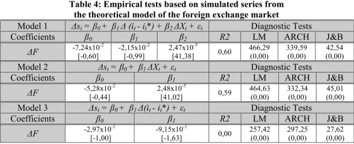
In a pioneered work, Evans and Lyons (2001, 2002) came up with an hybrid model based on private information and public information to explain exchange rate dynamics. The hybrid model takes the following form:

{ * 0 1 ( ) 2 t t t t t Private Information Public Information s

β β

i i

β

X

ε

∆ = + ∆ − + ∆ + 14243 (1)

With st, the (log of) the spot exchange rate (an increase in s is equal to an appreciation of the domestic currency); (it - it*), the interest rate differential between the domestic and the foreign country; Xt, the net cumulated order flow. ∆ stands for the first difference of the series. Macroeconomic fundamentals (here the interest rate differential (it - it*)) represents public information known by all agents. Order flows 2 Xt represent private information known by a minority of agents. Order flow is defined as the net of buyer- and seller-initiated currency transactions. Intuitively, order flow represents a willingness to back one's beliefs on future exchange rate dynamics, with real money.

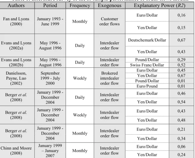
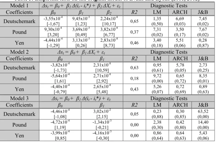
Evans and Lyons tested their model on the deutschemark/dollar, yen/dollar and pound/dollar in daily frequency from May 1996 to August 1996. They show that private information (order flows) explain at best 65 % of the variance of exchange rates. On the contrary, public information (the interest rate differential) only explains at best 5 % of the variance of exchange rates (a figure close to the ones obtained with traditional exchange rate models). Similar results can be found in the literature as shown in table 1.

2

Table 1: Literature survey of the in-sample performance of order flows models

Authors Period Frequency Exogenous Explanatory Power (R2)

Fan and Lyons (2000) January 1993 - June 1999 Monthly Customer order flows Euro/Dollar 0,16 Yen/Dollar 0,15

Evans and Lyons (2002a) May 1996 - August 1996 Daily Interdealer order flow Deutschemark/Dollar 0,67 Yen/Dollar 0,43

Evans and Lyons (2002b) May 1996 - August 1996 Daily Interdealer order flow Pound/Dollar 0,29 Swiss Franc/Dollar 0,52 Danielsson, Payne, Luo (2002) September 1999 - July 2000 Weekly Brokered interdealer order flow Euro/Dollar 0,45 Yen/Dollar 0,67 Pound/Dollar 0,01 Euro/Pound 0,01 Berger et al. (2008) January 1999 - December 2004 Daily Interdealer order flow Euro/Dollar 0,46 Yen/Dollar 0,54 Berger et al. (2008) January 1999 - December 2004 Weekly Interdealer order flow Euro/Dollar 0,43 Yen/Dollar 0,48 Berger et al. (2008) January 1999 - December 2004 Monthly Interdealer order flow Euro/Dollar 0,21 Yen/Dollar 0,34

Chinn and Moore (2008) January 1999 – January 2007 Monthly Interdealer order flow Euro/Dollar 0,06 Yen/Dollar 0,24

NB: The regression method used in the studies mentionned in table 1 is ordinary least squares (OLS)

Table 1 shows that the explanatory power of order flows model far exceeds the one of traditional models of exchange rate. For daily and weekly frequencies, the coefficients of determination (R2) spread between 30 % and 67 % (except for Danielsson et al. (2002)). At such frequencies, traditional exchange rate models usually provide R2 close to or less than 10 %. Beyond the explanatory performance of exchange rates, order flows provide also better exchange rate forecasts than traditional models. Numerous studies show that order flows models beat the random walk in the short run (Evans and Lyons (2001, 2002a, 2002b, 2005, 2006), Lindahl and Rime (2006), Rime et al. (2010)).

The results from order flows models have to be put into perspective. The relationship between order flows and exchange rate dynamics is strong at intradaily, daily and weekly frequencies but declines at lower frequencies. For example, table 1 shows that in Berger et al. (2008) order flows explain about 50 % of the variance of exchange rates at daily and weekly frequencies. At lower frequencies, for instance monthly frequencies, the R2 declines gradually and falls to 34 % for the yen/dollar exchange rate and to 21 % for the euro/dollar exchange rate. The same observation stands in Chinn and Moore (2008). Therefore the explanatory power of exchange rate variation by order flows models falls at monthly frequencies. In somes cases, the explanatory power comes even close to the one offered by traditional exchange rate models (see Chinn and Moore (2008)) while in other cases the explanatory power is still higher than the explanatory power of traditional exchange rate models based on

fundamentals (see Berger et al. (2008))3. Still, despite the relative fall in the explanatory power of order flows models at monthly frequencies, the literature review in table 1 provides evidence of the high explanatory and predictive performances by order flows models at short run horizons (from intradaily to weekly frequencies). As a result, one may wonder which types of information do order flows contain to justify such a high explanatory power of exchange rates at short horizons?

3. The informational content of order flows: a literature review

According to Lyons (2001), order flow contains private information. Private information can be split into three components: fundamental information, liquidity effects and portfolio balance effects.

Fundamental information includes private information about exchange rate fundamentals. For example, if a central bank intervenes in the foreign exchange market by transmitting a positive order flow to a market-maker, then this market-maker will infer a likely appreciation of the currency. Fundamental information is supposed to have a permanent effect on currency prices.

Inventory or liquidity effects refer to information about transfers of unwanted currency positions between market-makers. For instance, if a market-maker A has to absorb a large stock of currencies from a market-maker B, the market-maker A will bear more risks (mainly liquidity and valuation risks). As a result, the market-maker A will ask a higher risk premium (hence a lower price) to buy the currencies of market-maker B. This risk premium will only have a transitory effect on the price of the currency since it will disappear after the trade between the two market-makers. Thus inventory effects only have transitory effects on currency prices.

Portfolio balance effects relates to agents’ decisions independently of fundamental movements. For example, an import-export firm can operate in the market to convert foreign currencies in domestic currencies independently of fundamental movements. The effect of portfolio balance is assumed to be permanent on currency prices.

A lot of studies have analysed the informational content of order flows. The literature is split between two separate views: the strong flow centric view and the weak flow centric view.

The strong flow centric view states that order flows contains in majority fundamental information. Order flows are correlated with news about exchange rate fundamentals and have thus a permanent effect on currency prices (Ito et al. (1998), Rime (2000), Evans and Lyons (2001, 2002, 2005a, 2008), Love and Payne (2004), Marsh and O’Rourke (2005)).

Love and Payne (2004) base their study on intraday interdealer order flows on the euro/dollar, dollar/pound and pound/euro, from the 28th September 1999 to the 24th July 2000. They show that “even information that is publicly and simultaneously released to all

market participants is largely impounded into prices via the key micro-level price determinant - order flow”. Love and Payne find that between a half and two-thirds of price relevant

information is incorporated into prices via order flows.

Marsh and O’Rourke (2005) use daily customer order flows from August 2002 to June 2004 on bilateral exchange rates between the dollar, the euro, the pound and the yen. They

3

Recently, Carlini et al. (2010) show that in the long run (about 5 years), the cointegration relationship between order flows and stock prices is not significant. However by using more suitable tools, they show that order flows and stock prices are fractionnally cointegrated or even still cointegrated if we correct order flows by the volumes of transactions in the market.

show that inventory effects play a minor role in the informational content of order flows. A major role is attributed to fundamental effects. Particularly, when decomposing order flows by types of clients, they show that coefficients associated to leveraged firms such as hedge funds are very large compared to other flows (such as flows coming from unleveraged firm (mutual funds) and non-financial corporations (multinationals)). They conclude that flows coming from leveraged funds are more informative about fundamentals than flows coming from other customers4.

Evans and Lyons (2008) estimate an intraday model using interdealer order flows on the deutschemark/dollar market from May 1 to August 31, 1996. They show that roughly two-thirds of the total effect of macro news on the deutschemark/dollar exchange rate is transmitted via order flows. They claim that order flows contribute significantly to changing currency prices at all times, but that they contribute more to changing prices immediately after news arrivals about fundamentals.

Rime, Sarno and Sojli (2010) uses daily interdealer order flows for the euro, the pound

and the yen against the dollar between February 13, 2004 and February 14, 2005. They argue

that news about macroeconomic fundamentals are important determinants of order flows.

They find that “order flow is intimately linked to both news on fundamentals and to changes

in expectations about these fundamentals”.

According to the weak flow centric view order flows do not transmit private information about fundamentals in currency prices. Rather, order flows convey information about liquidity effects, temporary preferences and other demand shocks. Order flows have thus a transitory effect on asset prices. Evidence for the weak flow centric view is based on results provided by econometric analyses as well as survey studies.

Concerning survey studies, Cheung, Chinn and Marsh (2004) base their analysis on a sample of UK-based foreign exchange dealers in March/April 1998. They found that after analysing order flows, “traders do not vary their bid-ask spread either very often or for some

of the reasons thought important in the microstructure literature”. Microstructure theory

suggests that three main factors can lead traders to change their spreads: liquidity effects, portfolio balance effects and fundamental information. Cheung et al. (2004) add that “traders

were asked their reasons for changing their quoted spreads from the market convention and results suggest that the liquidity effect is dominant. This was confirmed in conversations with traders”.

In the same vein, Gehrig and Menkhoff (2006) sent questionnaires to professional market participants in Germany in July 1992. They show that “flows are more informative

about semifundamental private information. In other words, order flows contain information about short-term trading objectives or liquidity considerations of other traders that may affect short-term price movements, but that will not affect medium-term asset prices. Such information may be interim price relevant but irrelevant in the long run”. Gehrig and

Menkhoff add that “flow analysis does not seem to be used as a tool to learn about the

fundamental information”.

4

The view of Marsh and O’Rourke (2005) may be confirmed by Corsetti et al. (2001) who claim that a lot of operators believe that hedge funds have an informational advantage relative to the rest of the market concerning asset prices. However another interpretation of the high coefficients associated to order flows coming from hedge funds could be related to the fact that hedge funds speculate aggressively and thus produce huge movements in the market and hence in currency prices. Therefore order flows from hedge funds would be more related to speculative forces rather than to exchange rate fundamentals (Wei and Kim (1998)). Survey results among practitioners reinforce this argument since speculative forces are considered as a major determinant of exchange rates at short run horizons (Cheung and Wong (2000), Cheung and Chinn (2001) and Cheung, Chin and Marsh (2004)).

Concerning econometric studies, Breedon and Vitale (2004) analyse daily brokered interdealer trades in the dollar/euro exchange rate from August 2000 to mid-January 2001. They show that order flows provide above all, information about portfolio balance effects rather than information about macroeconomic fundamentals.

Froot and Ramadorai (2005) analyse a sample of daily institutional investor flows transactions for 18 exchange rates against the US dollar from June 1994 to February 2001. They show that order flows have a transitory impact on exchange rates and do not convey information about macroeconomic fundamentals to market-makers. “Flows appear to be

bound up with transitory currency under- and overreactions, but unrelated to the permanent component of exchange rate surprises. Yet, these exchange rate surprises are strongly related to important fundamental variables, as predicted by theory”.

Berger et al. (2008) analyse monthly interdealer order flows from January 1999 to December 2004 on the euro/dollar and the yen/dollar exchange rates. Their analysis points to an important role for liquidity effects in the relationship between order flows and exchange rates. They provide evidence that the relationship between order flows and exchange rates is strong at daily and weekly frequencies but weakens significantly from monthly frequencies.

Chinn and Moore (2008) analyse monthly interdealer order flows from January 1999 to January 2007 for the dollar/euro and dollar/yen exchange rates. They build an exchange rate model based on a combination of the traditional monetary model of exchange rate and the Evans-Lyons microstructure approach. They show that “cumulative order flow tracks liquidity

shocks and provides the ‘missing link’ to augmenting the explanatory power of conventional monetary models”.

This paper defends the idea that order flows contain information from both the strong and the weak flow centric view; but not solely. The article investigates inside the black box of order flows to disentangle the types of information contained in order flows. This question is becoming increasingly important as the literature has shifted the black box from understanding exchange rate determination to understanding order flow determination.

We build a theoretical model that considers all the information market agents can embed in currency prices. Our modeling approach integrates not solely the public and private information as in previous works (Bachetta and Van Wincoop (2006) and Evans (2010)) but also behavioural components affecting customers and dealers decisions. Our model thus merges two strands of the literature on exchange rates: behavioural exchange rate models and microstructure models of exchange rate. The global model takes account of heterogeneous agents (Frankel and Froot (1986)), the appearance of rumours (Dominguez and Panthaki (2006)), anchoring effects (Kahneman and Tversky (1974), Osler (2002)), status quo bias (Kahneman and Knetsch (1991), De Grauwe and Grimaldi (2008)) and the characteristics of the trading mechanism peculiar to the foreign exchange market (Lyons (1997, 2001)).

4. A theoretical model of the foreign exchange market 4.1 Hypotheses of the model

The model relies on two blocks. The first block is a behavioural model (De Grauwe and Grimaldi (2007)) that provides the characteristics of customers faced by dealers. We assume customers have heterogeneous expectations and are split between two main categories: chartists and fundamentalists. The second block is a microstructure model that represents the trading mechanism of the foreign exchange market. The microstructure model is a simultaneous-trade model that has a decentralised and multiple dealers structure as empirically observed in the foreign exchange market. Our model is based on Lyons (1997,

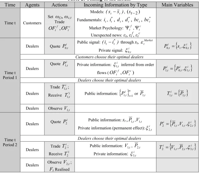
2001) with added elements from Bachetta and van Wincoop (2006). The microstructure model presents three advantages. First, it considers interdealer trading that accounts for two-thirds of the trades in the foreign exchange market. Secondly, it takes account of customer order flows as the primary source of private information for dealers. Besides, dealers learn about private information from other dealers through the observation of order flows. Thus the model assumes dealers have access to both public and private information. Thirdly, we suppose risk averse dealers as empirically observed in the foreign exchange market. Table 2 summarizes the timing of the model.

Table 2: Timing of the model

Time Agents Actions Incoming Information by Type Main Variables

Time t Customers Set ωf,t, ωc,t Trade f t OF ,OF_tc Models: (s_t −s_t ), (s_t−2) Fundamentals: i_t, i_t*, d_t, d*_t , bc_t, bc*_t Market Psychology: Ψ_tf ,Ψ_tc Unexpected news: εt, εtf, εtc Time t Period 1

Dealers Quote P₀i_,t Public signal: (i i )

* t t − through st, Market t ε Private signal: ξ₀i_,t

{

}

i t , t i t , s , P₀ = ξ₀

Customers choose their optimal dealers Dealers

Quote P₁i_{,t Private information:} i t ,

1

ξ inferred from order

flows (OF_tf ,OF_tc)

{

}

i t , i t , i t , P , P₁ = ₀ ξ₁

Dealers choose their optimal dealers

Dealers

Trade T₁i_t,;

Receive T₁'i_t, Public information:

{ }

n i i t , P 1 1 = or P1,t

{ }

,t i t , P T₁ = ₁ Dealers Observe V_1,t Time t Period 2 Dealers Quote i P₂ Public information: st ,P_1t,,V_1,t

Private information (permanent effect):ξ₂i_,t

{

}

i t , t , t , i , V , P P₂ = _{1 1} ξ₂

Dealers choose their optimal dealers Dealers Trade i T₂; Receive T₂'i Public information: V_1,t, P_2,t Private information: ξ₃i_,t

{

i

}

t , t , t , i , P , V T₂ = _{1 2} ξ₃ Dealers Observe V2,t; FtRealised

The timing of the model is described as follows. First, customers form their expectations based on their stock of information and their proper models of exchange rate determination. At the same time, dealers set their price5 based on public information. Customers then ask dealers about their listed price and choose their optimal dealer according to the prices set by dealers.

Trades in the microstructure model are split into two periods. In the first period the chosen dealers trade with their customers. Such dealers observe the flows coming from

5

Since in the foreign exchange market, the bid/ask spread is low due to a high degree of liquidity, we assume a bid/ask spread equal to zero in our model.

customers and try to infer the private information contained in customer order flows. In the second period, dealers trade among other dealers to adjust their stock of risky asset in two ways; either to satisfy the net demand of their customers or to take positions on currencies.

In our model the price of the currency is affected through two channels: a direct channel and an indirect channel. In the direct channel, the price of the currency can change with the arrival of public news even if there is no trade in the market. In the indirect channel, private information coming from customers affect currency prices through order flows6.

Sections 4.2 and 4.3 describe the structure of the model.

4.2 The behavioural model

The behavioural model is based on an heterogeneous agents structure (Frankel and Froot (1986), De Grauwe and Grimaldi (2007)). The model assumes customers can choose between two forecasting rules: a chartist rule and a fundamentalist rule. Fundamentalists forecast exchange rates based on the spread between the current exchange rate st and the fundamental exchange rates_t:

f t f t t t f t (s s ) s =−α − +α Ψ +ε ∆ _{+1 1 2} With {

α

₁,

α

₂ } > 0 (1.1) Thus if the exchange rate is over-appreciated (under-appreciated) relative to its fundamental value, fundamentalists will expect the currency to depreciate (appreciate). The parameter α1 represents the speed at which the exchange rate returns towards its fundamental value. The higher α1 the stronger the return force of exchange rates towards their fundamental value. The fundamental exchange rate s_t is determined by the interest rate differential between the two countries (it – it*):

) i i (

s_t = _t − _t* (1.2)

With i_t =i_t−1 +ε_t where i_t → N(0,σ_i2)and ε_t→ N(0,σ_ε2 ); i_t* =α*i_t*₋₁ +ε_t* where

85 0, * ₌

α

, * t i → N(₀,σ_i2_* )_and * t ε → N(₀, 2_* ) ε σ .7

Chartists interpolate past trends of exchange rates dynamics to forecast future currency prices: c t c t t c t s s =

β

+

β

Ψ +

ε

∆ _{+1 1}( ₋₂) ₂ With {

β

₁,

β

₂ } > 0 (2)

Thus when the exchange rate has appreciated (depreciated) in the past; chartists expect a further appreciation (depreciation) of the currency. Chartists thus magnify exchange rates movements. The parameter β1 represents the degree of interpolation. The higher β1, the larger the influence of past exchange rate dynamics on chartists’ forecasts.

6

The distinguishing feature between the two channels is easily understood with an example taken from Evans and Lyons (2008) and Evans (2009).

7

The interest rate differential has been filtered by a Hodrick-Prescott filter because we assume that the dynamics of the fundamental exchange rate are smooth over time.

The parameters Ψ and_tf Ψ represent the effects of collective psychology respectively _tc for fundamentalists and chartists. We assume two definitions for this component. First collective psychology is defined by the appearance of rumours (Dominguez and Panthaki (2006)) that counter past trends of the exchange rate:

∑

= − − = Ψ T i i t t , s T ₁ 1 1 (3.1)

Secondly, collective psychology is also materialised by the anchoring effect (Kahneman and Tversky (1974), Osler (2002)). When the exchange rate variation is lower than a constant (|∆st-1| ≤ c), the exchange rate fluctuates around a threshold value following a stable random walk (0 < θ < 1). Conversely, if the exchange rate variation is higher than a constant then the exchange rate wanders away from its current threshold and reaches a new threshold.    + + Λ + = Ψ − − t t t t t , s s

ε

θ

ε

θ

1 1 2 if c s c s t t > ∆ ≤ ∆ − − 1 1 (3.2)

With 0 < θ < 1 and Λ, a constant

The transition between the two states is driven by the following function: t t s ) ( F ε θ + = −1 1 .

The weight that market agents attribute to a given rule depends on the profitability of a particular rule. The more profitable a rule, the higher the weight agents attach to this rule. Chartist and fundamentalist weights are defined as:

)] exp( ) [exp( ) exp( ' , ' , ' , , t f t c t c t c γπ γπ γπ ω + = and )] exp( ) [exp( ) exp( ' , ' , ' , , t f t c t f t f

γπ

γπ

γπ

ω

+ = (4) Where ωf,t + ωc,t = 1 and 0 < γ < 1

The parameter γ represents the intensity at which agents revise their forecasting rules. When γ → ∞, agents choose the rule which proves to be the most profitable. Conversely, when γ → 0, agents keep the rule they are using and are insensitive to the profitability of this rule. Thus γ can be viewed as a represention of the status quo bias in agents’ behaviour. The

status quo bias highlighted by Kahneman and Knetsch (1991) means that when agents use a

given rule, they find it difficult to change for a different rule. We assume agents need some time to change their rule (γ = 0,2).

The profitability π'i,t of each rule is evaluated according to the profit π i,t and the risk

σ²i,t associated to a given rule:

The parameter µ represents the coefficient of risk aversion (we set µ = 5). The risk associated to a forecasting rule is defined as the variance of the forecasting error:

σ²i,t = [Eit-1(st) - st]² i = c, f (6) The profit π i,t related to a forecasting strategy is defined as the one-period earnings of investing one unit of domestic currency in the foreign asset:

π i,t = [st(1 + r*) - st-1(1 + r)]sgn[Eit-1(st)(1 + r*) - st-1(1 + r)] i = c, f (7) Where      < = = = > = 0 x if 1 -sgn[x] 0 x if 0 sgn[x] 0 x if 1 sgn[x]

Thus when agents forecast an appreciation of the foreign currency (an increase in st) they will invest in the foreign country. If this appreciation is realised then their profit is equal to the appreciation of the foreign currency, adjusted by the interest rate differential. Conversely, if the foreign currency depreciates (st decreases) agents will face a loss which equals the depreciation of the foreign currency, adjusted by the interest rate differential.

We assume fundamentals have an influence on exchange rate dynamics in the long run. More precisely, we assume that the external debt exerts a return force on currency prices such that the exchange rate returns towards its equilibrium value in the long run. The dynamics of the domestic (foreign) external debt d_t (d_t*) are defined as:

) s ( d ) i ( ) s ( bc d i d d_t = _t−1 + _{t t−1}+ _{t t−1} = 1+ _{t t−1}−

θ

_tfinal₋₁ (8.1) ) s ( d ) i ( ) s ( bc d i d d_t* = _t*₋₁ + *_{t t}*₋₁ + _t* _t−1 = 1+ _t* _t*₋₁ +

θ

_tfinal₋₁ (8.2) With d_t(d*_t ), the domestic (foreign) external debt; i_t(i_t*), the domestic (foreign) interest rate; bc_t(bc*_t ) the domestic (foreign) current account; s_t, the final exchange rate ; θ = 0,25; d_t =d_t−1 +

ε

_t where d_t→ N(0,

σ

_d2)and

ε

_t→ N(0,

σ

_ε2 ); d_t* =d*_t−1+

ε

_t*, where d_t*→

) , (

N 0

σ

_d2_* and

ε

_t*→ N(0,

σ

_ε2_* ) (initially we assume d_t=1 =0)

The stock of debt at time t is therefore equal to the stock of debt at time t-1 (d_t−1); plus the interest rate bear on the debt (i_td_t−1) and the current account balance at time t (bc_t). The current account is related to the exchange rate dynamics by an inverse relationship. Thus when the domestic currency appreciates, the current account worsens and vice versa. We assume also that fundamentalists do not take account of the effect of the external debt on the exchange rate in their rule. The external debt has here an external effect on exchange rate dynamics. In other words, the external debt influences the exchange rate dynamics outside the expectations of chartists and fundamentalists.

The expected exchange rate at time t+1 is obtained by aggregating agents’ forecasts in the market:

Et(∆st+1) = ωf,tEf,t(∆st+1) + ωc,tEc,t(∆st+1) – θ(dt-1 - dt-1*) ↔ Et(∆st+1) = - ωf,tψ(st - st*) + ωc,tβ∆st– θ(dt-1 - dt-1*) ↔ s_tMarket₊₁ = - ωf,tψ(st - st*) + ωc,tβ∆st– θ(dt-1 - dt-1*) +

ε

_{t 1}Market+ (9)

With θ = 0,25 and initially, d0 = 0

The following rules provide the link between the behavioural model and the microstructure model. Order flows from fundamentalists (OF_tf ) and chartists (OF_tc) are defined as: ) s ( F OF_tf = ∆ _tf₊₁ = N.∆s_tf₊₁ where OF_tf ∈ IN and       < = > 0 0 0 f t f t f t OF OF OF if       < ∆ = ∆ > ∆ + + + 0 0 0 1 1 1 f t f t f t s s s (10) ) s ( F OF_tc = ∆ _tc₊₁ = N.∆s_tc₊₁ where OF_tc∈ IN and       < = > 0 0 0 c t c t c t OF OF OF if       < ∆ = ∆ > ∆ + + + 0 0 0 1 1 1 c t c t c t s s s (11)

Therefore, when customers expect an appreciation of the currency, they will buy the currency. Conversely, when customers expect a depreciation of the currency, they will sell the currency. We assume customers select an optimal dealer. Customers willing to buy the risky asset choose the dealer that quotes the minimum price. Conversely, customers willing to sell the risky asset choose the dealer that quotes the maximum price. The total amount of customer order flows at time t is given by:

c t t f t t customers t OF ( )OF OF =

ω

+ 1−

ω

(12)

Table 3 decomposes the various types of information of the behavioural model.

Table 3: Decomposition of the information contained in the behavioural model

Public Fundamental Information Public Psychological Information Noise Fundamentalist Rule * t t * t t * t t t t,s ,i ,i ,d ,d ,bc ,bc s Ψ _tf

ε

_tf Chartist Rule st−2 c t Ψ c t

ε

Private Fundamental Information Private Psychological Information Noise Fundamentalist Rule

α

1(st −st ) f t Ψ 2

α

f t

ε

Chartist Rule

β

1(st 2− ) c t Ψ 2

β

c t

ε

The behavioural model contains four types of information: public fundamental information, private fundamental information, public psychological information and private psychological information.

Public fundamental information (s_t,s_t,i_t,i_t*,d_t,d_t*,bc_t,bc*_t ) deals with information concerning macroeconomic fundamentals. Every agent has access to public fundamental information.

Private fundamental information regroups information about fundamentals that has been analysed or processed by agents. The terms

α

₁(s_t −s_t )and

β

₁(s_{t 2−} ) describe the model of exchange rate determination in which agents believe. They are related to the internal psychology of agents.

Public psychological information (Ψ and _tf Ψ ) relates to information about market _tc psychology (or market agents behaviours) that can be observed by every agent. This type of information is associated to the external psychology of agents and can be illustrated by the anchoring effects or incoming rumours.

Private psychological information (

α

₂Ψ_tf and

β

₂Ψ_tc) defines the weight attributed by customers to the psychological component of exchange rate. Intuitively, this weight defines the degree of rationality of agents. Agents with no psychological components will be considered as more rational than agents who attibute a high weight to this component.

The parameter εtf (εtc) is a white noise that represents unexpected news or unexpected behaviours of fundamentalists (chartists). Therefore, the noise parameters can represent either public information or private information about fundamental or customers’ behaviours.

4.3 The microstructure model

We follow Lyons (1997) and model the trading mechanism of the foreign exchange market with a simultaneous-trade model with multiple dealers. We assume the existence of n dealers in the market. In this model, dealers are not solely market-makers (they match the supply and demand of currencies); they are also speculators (they take positions on currencies).

4.3.1 Period 1 of the microstructure model

Given their information set (public and private signal), dealers set their currency price based on the following rule:

Market t i t , t i t , s P₀ = +

ξ

₀ +

ε

(13)

Where

ξ

₀i_,t→ iidN(µ;σξ) and

ε

tMarket→ iidN(µ;σε)

The first price P₀i_,t set by dealers includes public information about fundamentals st, private information proper to the dealer

ξ

₀i_,t and unexpected news about fundamentals

ε

_tMarket.

i t ,

0

ξ

is interpreted as a private signal that dealers held concerning the future exchange rate dynamics. This private signal induces a difference among prices listed by dealers.

Equation (13) is the start of the direct channel of news incorporation into currency prices. Indeed, the price of the currency can change with the arrival of public news (through the terms

ε

_tMarket) even if there is no trade in the market (OF_tcustomers= 0).

Once dealers set their price, customers select their optimal dealers. Customers willing to buy the risky asset will choose the dealer that quotes the minimum price. Conversely, customers willing to sell the risky asset will choose the dealer that quotes the maximum price.

If 0 0 < > f t f t OF OF

, fundamentalists trade with dealer i such that:

{ }

_{{ }}

n i P Max P n i P Min P i i i i ∈ ∀ = ∈ ∀ = 0 0 0 0 If 0 0 < > c t c t OF OF

, chartists trade with dealer i such that:

{ }

{ }

P i n Max P n i P Min P i i i i ∈ ∀ = ∈ ∀ = 0 0 0 0 (14) Notice that some dealers receive orders from customers while other dealers do not. We thus face two cases. On the one hand, dealers that receive orders from customers have access to private information and include it into their price. On the other hand, dealers that do not receive any orders from customers do not have access to private information. Such dealers will learn about private information through the hot potato effect i.e. through interdealers order flows in period 2. Therefore customer order flow is the source of information asymmetry in this model. Thus private information will be reflected into prices only if it is not reflected in customer order flows and in interdealer order flows.

When dealers receive the information from customers, they will try to infer the private information contained in order flows. If dealers receive positive (negative) customer order flows OFtf + OFtc > 0 (OFtf + OFtc < 0), they will include a positive (negative) private signal

+

i t ,

1

ξ

(

ξ

₁i_,−_t ) in their quoted priceP₁i_,t. If dealers receive no customer order flows (OFtf = OFtc = 0), they receive no private signal from customers. We assume that the signal

ξ

₁i_,t extracted by dealers from customer order flows follows a white noise process. The quoted price P₁i_,t by dealers after trades with customers is thus given by:

     + = − + 0 1 1 0 1 i t , i t , i t , i t , P P

ξ

ξ

if 0 0 0 = + < + > + c t f t c t f t c t f t OF OF OF OF OF OF

Where

ξ

₁i_,t→ iidN(µ;σε) and

[ ]

[

]

   − ∈ ∈ − + 0 1 1 0 1 1 , , i t , i t ,

ξ

ξ

(15)

Dealers quote their price simultaneously and independently. Quoted price are observable and available to all dealers. Each quote is a single price at which the dealer agrees both to buy and sell. Equation (15) is the start of the indirect channel in which dispersed or private information coming from customers affect currency prices through order flows, based on the term

ξ

₁i_,t.

We define the demand for the risky asset by dealers or the desired stock of currency in period 1 for dealer i D₁i_,tby:

i t , D₁ =a₁s_t +a₂

ξ

₀i_,t +a₃i

ξ

₁i_,t −a₄P_1,t (16) With d i a

µ

γ

1 3 = , 0 < {a1,a2,a4}< 1 and

∑

= = N i i t , t , P N P 1 1 1 1

Therefore dealers have access to both public and private information sources. Their demand for the risky asset depends on public information st (the higher st, the more appreciated the value of the stock of risky asset, the higher the demand for the risky asset); private information coming from customer order flows

ξ

₁i_,t(the higher

ξ

₁i_,t, the higher the incentive for dealers to invest in the risky asset); the private signal that dealers held on the future exchange rate dynamics i

t , 0

ξ

(the higher i t , 0

ξ

, the higher the incentive for dealers to invest in the risky asset); and the average price set by dealers in period 1 P_1,t (the higher the price of the risky asset, the lower the demand for the risky asset).

Dealers are also speculators in this model. They benefit from the information contained in the received customer orders to take speculative positions. The term γ1i takes account of the speculative dimension of dealers. This term acts as a leverage effect on the demand for currencies by dealers. We assume that the willingness to buy or sell currencies for dealers depends on the amount bought or sold by their customers. If dealers receive customer orders higher than the average order flows received in the past from customers, they will buy a higher amount of currencies. Conversely, if dealers receive customer orders lower than the average order flows received in the past from customers, they will buy a lower amount of currencies. The same reasoning holds when selling currencies. Thus, the willingness to buy/sell currencies by dealer i is defined by the term γ1i such as:

   > < < = 1 1 0 1 1 1 i i i

γ

γ

γ

if customer t customer t customer t customer t F O OF F O OF > < (17)

The parameter µd represents the degree of risk aversion of dealers: if µd < 1, dealers are risk lover; if µd > 1, dealers are risk averse; if µd = 1, dealers are risk neutral.

Beyond their role of speculators, dealers are also market-makers. They match the demand and supply of currencies by customers. We define the dealer i trading rule T₁i_t, in period 1 as: i t , i t , i t , D C T₁ = ₁ + ₁ + E[ T₁'_,i_t /Ω ] ₁i_,t (18) The term _Ti 1 depends on i D₁, _Ci 1 and E[ i i T' ₁

1 / Ω ]. Assume initially that the stock of

risky assets for dealers is equal to zero. The term _Ti

1 is the necessary amount of orders that

dealers have to pass to other dealers to satisfy their own demand of risky asset given orders coming from customers and orders from other dealers. The termC₁i represents customer order flows addressed to dealer i. Customers will be net buyers if C₁i > 0. Conversely, customers will be net sellers if C₁i < 0. Obviously, C₁i = OF +_tf OF . If the dealer does not receive any _tc

orders from customers, then OF_tf =OF_tc =0 and C₁i= 0. As dealers’ trades are simultaneous,

E[T₁'i / Ω ] as: E[₁i T₁'i/ Ω ] = ₁i T_{2 −}'i_{,t 1}+

ε

_ti. The term T_{2 −}'i_{,t 1} represents the net flows received by dealer i from other dealers in period 2 8. The term D₁i_,t is the desired stock of currencies by dealer i.

The definition of order flows by dealer i T₁i_t, in period 1 is given by9: i t , i t , i t , D C T₁ = ₁ + ₁ + E[ T₁'_,i_t /Ω ] ₁i_,t (19) <=> T₁i_,t = a₁s_t +a₂

ξ

₀i_,t +a₃i

ξ

₁i_,t −a₄P_1,t+ (OF + _tf OF ) + _tc T_{2 −}'_,i_{t 1}+

ε

_ti (20) Dealers then choose to trade with their optimal dealers. Buyer dealers will buy currencies at the lowest price. Seller dealers will sell currencies at the highest price:

If    < > 0 0 1 1 i t , i t , T T

the dealer i trades with dealer j such as:

{ }

_{{ }}

n j P Max P n j P Min P j t , j t , j t , j t , ∈ ∀ = ∈ ∀ = 1 1 1 1 (21)

The net cumulated interdealer order flows in period 1 amount to:

∑

= = n i i t , t , T V 1 1 1 (22)

4.3.2 Period 2 of the microstructure model

In period 2, dealers trade between each other. Their trades are based on private information contained in order flows. Dealers start to revise their quoted price given their updated stock of information. We assume that the price quoted by dealers in period 2 is linked to the latest market quote P_1,t and to the net interdealer order flows in period 1 V_1,t. This assumption gives more stability to the model. Hence:

     + = − + 0 2 2 1 2 i t , i t , t , i t , P P

ξ

ξ

if 0 0 0 1 1 1 = < > t , t , t , V V V

Where

ξ

₂i_,t→ iidN(µ;σε) And

[ ]

[

]

   − ∈ ∈ − + 0 1 1 0 2 2 , , i t , i t ,

ξ

ξ

(23)

Once dealers have set their price in period 2, they define their net demand for currencies in period 2 D₂i_,taccording to the following relationship:

i t , d i t , t , t d i t , (bs bV b P ) D₂ 1 _{1 2 1 3 2} 2

ξ

₃

µ

γ

µ

+ − + = (24) With

∑

= = N i i t , P N P 1 2 2 1 , 0 < {b1,b2,b3}< 1 and b1 > b3 8

Initially, we set T_{2 −}'_,i_{t 1}=0 and E[ T₁'_,ti /Ω₁i] =

ε

_ti.

9

And      = − + 0 3 3 3 i t , i t , i t,

ξ

ξ

ξ

if i ' t , i ' t , i ' t , i ' t , i ' t , i ' t, T T T T T T 1 1 1 1 1 1 = > <

where

ξ

₃i_,t→ iidN(µ;σε) and

[ ]

[

]

   − ∈ ∈ − + 0 1 1 0 3 3 , , i t , i t,

ξ

ξ

(25)

Hence the demand for currencies in period 2 D₂i_,tdepends on public information st (the higher st, the more appreciated the value of the stock of risky asset, the higher the demand for the risky asset); interdealer order flows V_1,tobserved by dealers at the end of period 1 (the more positive V_1,t, the more appreciated the value of the stock of risky asset, the higher the demand for the risky asset); the average price set by dealers in period 2 P_2,t (the higher the price of the risky asset, the lower the demand for the risky asset); private information coming from dealers that received customer order flows in period 1

ξ

₃i_,t(the higher

ξ

₃i_,t, the higher the incentive for dealers to invest in the risky asset). Indeed, in period 2, dealers infer private information

ξ

₃i_,t from customer order flows through order flows coming from dealers that had traded with customers in period 1. Recall that the only way dealers can learn about private information from other dealers is through the observation of interdealer order flows.

Dealers are also speculators. The term γ2 takes account of the speculative dimension of dealers. This term acts as a leverage effect on the demand for currencies by dealers. We assume the willingness to buy or sell the risky asset for a dealer depends on the amount bought or sold by their dealers’ counterparts. Therefore, if a dealer receives orders higher than the average flows received in the past, he will buy a higher amount of risky asset. Conversely, if a dealer receives orders lower than the average flows received in the past; he will buy a lower amount of risky asset. The same reasoning holds when selling currencies. The term γ2i defines the willingness to buy/sell the risky asset:

   > < < = 1 1 0 2 2 2 i i i

γ

γ

γ

if _'i t , i ' t , i ' t , i ' t, T T T T 1 1 1 1 > < (26)

The parameter µd represents the degree of risk aversion of dealers: if µd < 1, dealers are risk lover; if µd > 1, dealers are risk averse; if µd = 1, dealers are risk neutral.

The dealer trading rule in period 2 is defined as follows: − + − = 'i t , i t , i t , i t , D D T T_{2 2 1 1} E[T₁'_,i_t /Ω ] + E[ ₁i_,t T₂'i_,t /Ω ] i_2,t (27) The term T₂idepends on D₁i , D₂i , T₁'_t,i , E[ T₁'i/ Ω ] and E[ ₁i T₂'i /Ω ]. The flows i₂

(_Di _Di

1

2 − )represent a revision by dealer i of the amount invested in currencies. The term

(_Di _Di

1

2 − ) is interpreted as an inventory effect. The inventory effect in turn triggers the hot

potato effect. Hence agents pass their undesired positions to other dealers in the market through the termT₂i. Trades in period 2 depend also on the error made by a dealer on the expected flows coming from other dealers (T₁'i −E[T₁'i / Ω ])₁i 10 in period 1 and on the expected

10

order flows to be received in period 2 (E[ T₂'i/ Ω ]). The expected flows from other dealers by i₂ a dealer i is simply equal to flows received by a dealer i in period 1, plus a noise:

E[T₂'i / Ω ] = i₂ '_,i_{t t}i i T +ε

∑

= 1 3 1 With ε_ti→ iidN(µ;σε) (28)

Therefore, the definition of order flows by a dealer i in period 2 _Ti

2 is given by: = i T₂ i_,t d i t , t, t d ) P b V b s b ( 2 ₃ 2 3 1 2 1 1 ξ µ γ µ + − + -( i ' t , T_{2 −1}+ ε_ti)+ ( 'i _ti i T +ε

∑

= 1 3 1 ) (29)

Dealers then choose to trade with their optimal dealer. Buyer dealers will buy currencies at the lowest price. Seller dealers will sell currencies at the highest price:

If    < > 0 0 2 2 i t, i t , T T

the dealer i trade with dealer j such as:

{ }

_{{ }}

j i , n j P Max P j i , n j P Min P j t , j t , j t , j t , ≠ ∈ ∀ = ≠ ∈ ∀ = 2 2 2 2 (30)

The net cumulated interdealer order flows in period 2 amount to:

∑

= = n i i t , T V 1 2 2 (31)

The final value F of the risky asset in period 2 is given by: _t

∑

= + = = n i t i t P s n F 1 1 2 1 (32)

4.4 Stochastic simulations of the model

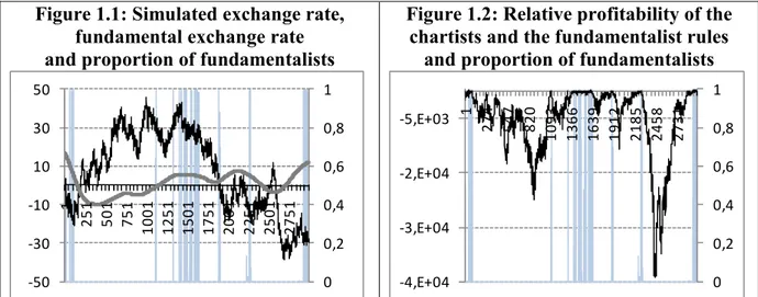
We simulate the model over 3000 periods with 50 dealers in the market11. Figure 1.1 shows the dynamics of the simulated exchange rate, the fundamental exchange rate and the proportion of fundamentalists in the market. Figure 1.2 show the relative profitability of the chartists and the fundamentalist rules and the proportion of fundamentalists.

11

Figure 1.1: Simulated exchange rate, fundamental exchange rate and proportion of fundamentalists

0 0,2 0,4 0,6 0,8 1 -50 -30 -10 10 30 50 1 2 5 1 5 0 1 7 5 1 1 0 0 1 1 2 5 1 1 5 0 1 1 7 5 1 2 0 0 1 2 2 5 1 2 5 0 1 2 7 5 1

Figure 1.2: Relative profitability of the chartists and the fundamentalist rules

and proportion of fundamentalists

0 0,2 0,4 0,6 0,8 1 -4,E+04 -3,E+04 -2,E+04 -5,E+03 1 2 7 4 5 4 7 8 2 0 1 0 9 3 1 3 6 6 1 6 3 9 1 9 1 2 2 1 8 5 2 4 5 8 2 7 3 1

NB: For figure 1.1, the black line represents the simulated exchange rate F (left scale); the grey line represents the fundamental exchange rate s (left scale); the blue margins represents periods in which fundamentalists dominate the market ω(right scale). For figure 1.2, the black line represents the relative profitability between the chartits rule and the fundamentalist rule (π'f,t - π'c,t); the blue margins represents periods in which fundamentalists dominate the market ω(right scale).

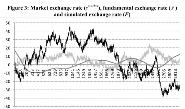
From figure 1.1, we observe that in the short run, there is a persistent gap between the simulated exchange rate F and its fundamental value s . Over the long run, the simulated exchange rate returns towards its fundamental value. The heterogeneity of behaviours in the market or equivalently the use of different models by agents explains the disconnection of the market exchange rate from its fundamental value. When chartists dominate the market (white margins), the exchange rate wanders away from its fundamental value. Conversely, when fundamentalists dominate the market (blue margins), the exchange rate returns towards its fundamental value.

As shown in figure 1.2 the domination of a given type of agent in the market depends on the the profitability of its proper rule. If the profitability of the chartist rule is higher than the profitability of the fundamentalist rule, chartists dominate the market. Conversely, when the fundamentalist rule becomes more profitable than the chartist rule, fundamentalists dominate the market.

Figure 2.1 and 2.2 shows the dynamics of the simulated exchange rate with respectively the ones of customer order flows and interdealer order flows.

Figure 2.1: Simulated exchange rate and customer order flows

-200 -100 0 100 200 300 -60 -40 -20 0 20 40 60 1 2 7 4 5 4 7 8 2 0 1 0 9 3 1 3 6 6 1 6 3 9 1 9 1 2 2 1 8 5 2 4 5 8 2 7 3 1

Figure 2.2: Simulated exchange rate and interdealer order flows

-1,E+06 -9,E+05 -4,E+05 1,E+05 6,E+05 1,E+06 2,E+06 2,E+06 -60 -40 -20 0 20 40 60 1 2 7 4 5 4 7 8 2 0 1 0 9 3 1 3 6 6 1 6 3 9 1 9 1 2 2 1 8 5 2 4 5 8 2 7 3 1

NB: For figure 2.1, the black line represents the simulated exchange rate F (left scale); the dark grey line represents customer order flows OFcustomer (right scale). For figure 2.2, the black line represents the simulated exchange rate F (left scale); the light grey line represents interdealer order flows V2 (right scale).

From figures 1.1, 2.1 and 2.2, we obverse that the model replicates three stylised facts observed empirically in the foreign exchange market.

First of all, simulations in figures 2.1 and 2.2 confirm the close link between exchange rate dynamics and cumulative order flows at short and long horizons. The coefficient of correlation between the simulated exchange rate and customer order flows (interdealer order flows) amounts to 99,47 % (respectively 98,42 %). This result comes in line with the empirical observations by microstructure theorists (Lyons (2001), Evans and Lyons (2001, 2002a, 2002b), Rime et al. (2010) to cite a few).

Secondly, the amount of interdealer order flows is larger than the amount of customer order flows. This fact is due to the hot potato effect. This phenomenon describes the fact that with the incoming stock of new information dealers revise their demands of currencies. Revisions in their willing stock of currencies induce inventory imbalances or undesired stock of currencies. Dealers get rid of these inventory imbalances by passing them to other dealers. As a result, inventory imbalances are passed from dealers to dealers in the market. These trades of unwanted positions inflate the amount of flows between dealers in the market. These trades further magnify the amount of interdealer order flows relative to the initial amount of customer order flows. In the model, the hot potato effect appears in period 2 where dealers trade between each other. The hot potato effect is defined through the term _Ti

2 by the

inventory effect or equivalently the revision of undesired positions on currencies (_Di _Di

1 2 − ).

Such inventory effects are an important feature of models willing to address trading mechanism in the foreign exchange market. Indeed, empirically, the hot-potato effect represents 60 % of the trades between agents in the foreign exchange market (Lyons (2001)).

Thirdly, figures 1.1, 2.1 and 2.2 show that in the short run, the simulated exchange rate is disconnected from its fundamentals but not from order flows. However, in the long run, the dynamics of the simulated exchange rate returns towards its fundamental value and is still highly correlated with order flows. This result comes in lines with the one from the theoretical work by Bachetta and van Wincoop (2006) and the empirical work by Berger et al. (2008).