HAL Id: tel-02173727
https://pastel.archives-ouvertes.fr/tel-02173727
Submitted on 4 Jul 2019
HAL is a multi-disciplinary open access
archive for the deposit and dissemination of sci-entific research documents, whether they are pub-lished or not. The documents may come from teaching and research institutions in France or abroad, or from public or private research centers.
L’archive ouverte pluridisciplinaire HAL, est destinée au dépôt et à la diffusion de documents scientifiques de niveau recherche, publiés ou non, émanant des établissements d’enseignement et de recherche français ou étrangers, des laboratoires publics ou privés.
On the conditioning of �process-based channelized
meandering reservoir models on well data
Anna Bubnova
To cite this version:
Anna Bubnova. On the conditioning of �process-based channelized meandering reservoir models on well data. Earth Sciences. Université Paris sciences et lettres, 2018. English. �NNT : 2018PSLEM055�. �tel-02173727�
Préparée à MINES ParisTech
Sur le conditionnement des modèles génétiques de
réservoirs chenalisés méandriformes
à des données de puits
On the conditioning of process-based channelized
meandering reservoir models on well data
Soutenue par
Anna BUBNOVA
Le 11 décembre 2018
Ecole doctorale n° 398
Géosciences, Ressources
Naturelles et Environnement
(GRNE)
Spécialité
Géosciences et géoingénierie
Composition du jury :
Peter HUGGENBERGER Professeur,Université de Bâle (Suisse) Président
Daniel GARCIA Maître de Recherche,
Ecole des Mines de Saint-Etienne Rapporteur
Pauline COLLON
Maître de Conférence, HDR,
ENSG-Université de Lorraine Rapporteur
Bernard GUY Docteur d'Etat,
Ecole des Mines de Saint-Etienne Examinateur
Sur le conditionnement des
modèles génétiques de réservoirs chenalisés méandriformes à des données de puits
par Anna Bubnova
Résumé
Les modèles génétiques de réservoirs sont construits par la simulation des principaux processus de sédimentation dans le temps. En particulier, les modèles tridimensionnels de systèmes chenalisés méandriformes peuvent être construits à partir de trois processus principaux : la migration du chenal, l’aggradation du système et les avulsions, comme c’est réalisé dans le logiciel Flumy pour les environnements fluviatiles. Pour une utilisation opérationnelle, par exemple la simulation d'écoulements, ces simulations doivent être conditionnées aux données d'exploration disponibles (diagraphie de puits, sismique, …). Le travail présenté ici, basé largement sur des développements antérieurs, se concentre sur le conditionnement du modèle Flumy aux données de puits.
Deux questions principales ont été examinées au cours de cette thèse. La première concerne la reproduction des données connues aux emplacements des puits. Cela se fait actuellement par une procédure de "conditionnement dynamique" qui consiste à adapter les processus du modèle pendant le déroulement de la simulation. Par exemple, le dépôt de sable aux emplacements de puits est favorisé, lorsque cela est souhaité, par une adaptation des processus de migration ou d'avulsion. Cependant, la manière dont les processus sont adaptés peut générer des effets indésirables et réduire le réalisme du modèle. Une étude approfondie a été réalisée afin d'identifier et d'analyser les impacts indésirables du conditionnement dynamique. Les impacts ont été observés à la fois à l'emplacement des puits et dans tout le modèle de blocs. Des développements ont été réalisés pour améliorer les algorithmes existants. La deuxième question concerne la détermination des paramètres d’entrée du modèle, qui doivent être cohérents avec les données de puits. Un outil spécial est intégré à Flumy - le "Non-Expert User Calculator" (Nexus) - qui permet de définir les paramètres de simulation à partir de trois paramètres clés : la proportion de sable, la profondeur maximale du chenal et l’extension latérale des corps sableux. Cependant, les réservoirs naturels comprennent souvent plusieurs unités stratigraphiques ayant leurs propres caractéristiques géologiques. L'identification de telles unités dans le domaine étudié est d'une importance primordiale avant de lancer une simulation conditionnelle avec des paramètres cohérents pour chaque unité. Une nouvelle méthode de détermination des unités stratigraphiques optimales à partir des données de puits est proposée. Elle est basée sur la Classification géostatistique hiérarchique appliquée à la courbe de proportion verticale (VPC) globale des puits. Les unités stratigraphiques ont pu être détectées à partir d'exemples de données synthétiques et de données de terrain, même lorsque la VPC globale des puits n'était pas visuellement représentative.
On the conditioning of
process-based channelized meandering reservoir models on well data
by Anna Bubnova
Abstract
Process-based reservoir models are generated by the simulation of the main sedimentation processes in time. In particular, three-dimensional models of meandering channelized systems can be constructed from three main processes: migration of the channel, aggradation of the system and avulsions, as it is performed in Flumy software for fluvial environments. For an operational use, for instance flow simulation, these simulations need to be conditioned to available exploration data (well logging, seismic, …). The work presented here, largely based on previous developments, focuses on the conditioning of the Flumy model to well data.
Two main questions have been considered during this thesis. The major one concerns the reproduction of known data at well locations. This is currently done by a "dynamic conditioning" procedure which consists in adapting the model processes while the simulation is running. For instance, the deposition of sand at well locations is favored, when desired, by an adaptation of migration or avulsion processes. However, the way the processes are adapted may generate undesirable effects and could reduce the model realism. A thorough study has been conducted in order to identify and analyze undesirable impacts of the dynamic conditioning. Such impacts were observed to be present both at the location of wells and throughout the block model. Developments have been made in order to improve the existing algorithms.
The second question is related to the determination of the input model parameters, which should be consistent with the well data. A special tool is integrated in Flumy – the Non Expert User calculator (Nexus) – which permits to define the simulation parameters set from three key parameters: the sand proportion, the channel maximum depth and the sandbodies lateral extension. However, natural reservoirs often consist in several stratigraphic units with their own geological characteristics. The identification of such units within the studied domain is of prime importance before running a conditional simulation, with consistent parameters for each unit. A new method for determining optimal stratigraphic units from well data is proposed. It is based on the Hierarchical Geostatistical Clustering applied to the well global Vertical Proportion Curve (VPC). Stratigraphic units could be detected from synthetic and field data cases, even when the global well VPC was not visually representative.
Hierarchical Clustering, Geostatistics, Process-based models, reservoirs, conditional
simulations
Acknowledgments
Firstly, I would like to express my sincere gratitude to my thesis advisors: Jacques Rivoirard
and Isabelle Cojan. Thanks to you, I have acquired the skills that will help me during my
professional life. I am also grateful to Flumy team: Martin, Jean-Louis and especially to
Fabien Ors – for your help during the years of my work.
I would like to thank the members of my thesis committee – Peter Huggenberger, Daniel
Garcia, Pauline Collon, Bernard Guy and Simon Lopez.
I would also like to acknowledge our Flumy consortium partners: ENI and ENGIE.
My sincere thanks go to my dear colleagues from the Center of Geosciences MINES
ParisTech: Helene, Christian, Laure, Jihane, Ricardo, Marine, Jean, Emilie, Xavier, Marine,
Robin, Nathalie, Isabelle et Sylvie, Didier, Gaelle, Chantal, Nicolas and Thomas. It was great
to have an opportunity to work in your team.
A very special gratitude goes out to POE Big Data team: Dinh, Avish, Razan, Catalina, Maria
Angelica, Sara, Tristan, Zishan and Theo. Thanks to you all for your support during the last
months.
And finally, last but no means least, I would like to thank my friends and family.
Спасибо
моей семье и друзьям – любимым маме и бабушке, Маше, Саше, Сереже, Оле, Аленке,
Ксюше и Маше. Я всегда чувствую вашу поддержку, даже на расстоянии.
SUMMARY
Summary
ABBREVIATIONS
XI
LIST OF FIGURES
XV
LIST OF TABLES
XXV
INTRODUCTION
1
1
FLUMY MODEL FOR MEANDERING FLUVIAL SYSTEMS
5
1.1 Meandering Fluvial Systems 5
1.1.1 Modern systems 5
1.1.1.1 Meandering channel geometry 6
1.1.1.2 Evolution of the meander loops 6
1.1.1.3 Overbank flow sediments 7
1.1.1.4 Levee breaches 8
1.1.2 Fossil systems 9
1.2 Flumy model 12
1.2.1 Migration 14
1.2.2 Aggradation 15
1.2.3 Levee breaches and avulsions 16
1.2.4 Conclusion 18
1.3 Flumy – Non-Expert User Calculator (Nexus) 20
1.3.1 Key Nexus parameters 20
1.3.2 Use of the Nexus 21
2
CONDITIONING MEANDERING SYSTEMS
25
2.1 Review of conditioning techniques 25
2.1.1 1D conditioning 26 2.1.1.1 Static conditioning 26 2.1.1.2 Dynamic conditioning 30 2.1.2 2D conditioning 32 2.1.3 3D conditioning 33 2.1.3.1 Geomorphological models 33 2.1.3.2 Boolean models 35
SUMMARY
viii
2.2.4 Concept of Active Level and Active Brick 45
2.2.5 Adaptation of migration 47
2.2.6 Adaptation of avulsions 47
2.3 Conditioning in Flumy: initial algorithms 49
2.3.1 Update Active Level 49
2.3.2 Adaptation of migration 53
2.3.2.1 Brief algorithm presentation 53
2.3.2.2 Erodibility correction according to the three lithofacies classes 56
2.3.3 Adaptation of avulsions 60
2.3.4 Conclusion 65
3
TOWARDS A FINER CONDITIONING
67
3.1 Tools for evaluation of conditioning results 67
3.1.1 Conditioning statistic table 68
3.1.2 Non-conditional and conditional simulation cross-section comparison 68
3.1.3 Sand Proportion Map 69
3.2 Reproducing lithofacies at wells 69
3.2.1 Single-facies well 69
3.2.1.1 Non-channelized facies 70
3.2.1.2 Channelized facies 73
3.2.1.3 Conclusion 78
3.2.2 Multi-facies well 78
3.2.2.1 Low sand proportion 79
3.2.2.2 High sand proportion 81
3.2.2.3 Sheet type sandbodies 83
3.2.2.4 Conclusion 84
3.2.3 Multiple wells 85
3.2.3.1 Four synthetic wells 85
3.2.3.2 Four simulated wells 88
3.2.4 Conclusions 91
3.3 Resulting sand spatial distribution 92
3.3.1 Influence of flow direction 92
3.3.2 Case of aligned wells 95
3.3.2.1 Wells aligned along the flow 95
3.3.2.2 Wells aligned perpendicularly to the flow 96
3.3.3 Conclusions 99
3.4 Revised conditioning techniques 100
3.4.1 Revised treatment of thin lithofacies data 101
3.4.2 Refactoring of updating Active Level 102
3.4.3 Improvement of migration adaptation 115
3.4.4 Improvement of avulsions adaptation 115
3.4.5 Blocking aggradation 116
SUMMARY
3.5 Impact of the revised conditioning techniques 118
3.5.1 Reproducing facies at wells 119
3.5.1.1 Multi-facies well 119
3.5.1.2 Multiple wells 125
3.5.1.3 Conclusion 132
3.5.2 Resulting sand spatial distribution 133
3.5.2.1 Influence of flow direction 134
3.5.2.2 Wells aligned along the flow 135
3.5.2.3 Wells aligned perpendicular to the flow 136
3.5.3 Identified issue in the vicinity of wells 139
3.5.3.1 Sand distribution vs repulsion algorithm in the well vicinity 140
3.5.3.2 Uniform sand distribution during conditioning 142
3.5.3.3 Conclusion 143
3.5.4 Conclusion 144
3.6 Conclusions 145
4
AUTOMATIC DETERMINATION OF SEDIMENTARY UNITS FROM WELL
DATA
147
4.1 Introduction 149
4.2 Method 152
4.2.1 Hierarchical clustering overview 152
4.2.2 Geostatistical Hierarchical Clustering (GHC) 154
4.2.3 Adaptation of the GHC to well data 154
4.3 Material 156
4.3.1 The Loranca meandering succession 156
4.3.2 The Flumy model 157
4.4 Results 158
4.4.1 First synthetic case: contrasted units 159
4.4.2 Second synthetic case: less contrasted units 160
4.4.3 Loranca case study 162
4.5 Conclusions and perspectives 165
5
CONCLUSIONS AND PERSPECTIVES
167
5.1 General Discussion 168
ABBREVIATIONS
Abbreviations
Flumy facies
and colorscales
ABBREVIATIONS
xii
Abbreviations used for dynamic conditioning:
AB Active Brick;
AL Active Level;
botab active brick bottom elevation; topab active brick top elevation;
twat top water elevation (top elevation of the channel in a Wet Well);
zb well bottom elevation;
zt well top elevation;
zdep bottom elevation of the last deposit remaining part to be validated;
zdom top elevation of the last deposit (corresponds to the floodplain elevation at the well);
Other abbreviations:
GHC Geostatistical Hierarchical Clustering; MPS Multiple Point Statistics;
NEXUS Non Expert User Calculator; PGS Plurigaussian Simulations; SIS Sequential Indicator Simulations; TIN Triangulated Irregular Networks;
LIST OF FIGURES
List of figures
Figure 1. (a) A meandering river in Siberia. Image Credit: Ólafur Ingólfsson, http://www3.hi.is/~oi/; (b) Carson River (USA) during an overbank flood (https://nevada.usgs.gov/crfld/floodtypes.htm) (c) Lateral accreting sand bars in a meander loop (from Hickin, 1974); (d) aerial view of a point bar (Allier river, France), pink shaded area corresponds to the crest height that are quickly
colonized by vegetation (from Deleplancque, 2016) ... 5 Figure 2. (a) Cross-section in a straight reach mean bankfull depth; (b) cross-section at the bend apex
max bankfull depth (From Held, 2011). ... 6 Figure 3. Illustration of a meander loop by neck cutoff (a) and chute cutoff (b) (Dieras, 2013); (c) map of the Mississippi channel belt built over some ten thousand years (Fisk, 1944); (d) satellite photo of the Jutaï River (Amazon, North Brazil) extracted from Google Earth. This picture shows the meandering belt formed by a high sinuosity river, within which meander intersections also cause the formation of lakes and dead arms. ... 7 Figure 4. (a) Scheme of overflow sediments formation; (b) the Red River during the 1997 flood,
viewed southwards from near St. Norbert, Manitoba (Canada). Courtesy Geological Survey of Canada (up), and Missouri River flood (2018 Scripps Media, Inc.) (below) ... 8 Figure 5. (a) Levee breach along the Mississippi River (source:
http://www.20min.ch/ro/news/monde/story/14925437); (b) Crevasse splay, Columbia River, Canada (source: http://www.seddepseq.co.uk/) ... 9 Figure 6. Point bar of around 3m height, showing the lateral extension of 18-20m ... 9 Figure 7. Levee deposits interrupted by a crevasse splay (thicker bed with a coarser grain size) in relief
in the section. Hammer, 0.4m for scale ... 9 Figure 8. Paleosol ... 10 Figure 9. Oxbow lake with orange clayey deposits and white facies limestone bed. The person is
standing on the toe of the last point bar set before the loop abandonment ... 10 Figure 10. Incision at the base of the sandstone cliff, corresponding to an avulsion ... 10 Figure 11. Isolated sandbodies in the alluvium deposits during a period of high aggradation rate; on
top – amalgamated sandbodies during a period of low aggradation rate. ... 11 Figure 12. Schematic illustration of principal elements of a Meandering Fluvial System illustrated
LIST OF FIGURES
xvi Figure 17. Flumy channel cross-section example. In blue – the channel with the water inside, from red
to yellow color – deposited sandy Point Bars from the old to new deposits ... 15
Figure 18. Flumy valley cross-section scheme (vertical scale exaggeration) ... 16
Figure 19. Overbank Flood in Flumy (cross-section and 3D view) ... 16
Figure 20. Flumy cross-section with wetland depositions on the floodplain ... 16
Figure 21. A local (left) and a regional (right) avulsion in Flumy, 3D view... 17
Figure 22. New channel path examples (resulting from a regional avulsions) ... 17
Figure 23. Variability of Flumy results in function of aggradation rate and avulsions period (Flumy cross-section view of 16 different scenarios) ... 19
Figure 24. Illustration of Isbx possible values and its influence on the simulation results (Flumy aerial 2D view) ... 21
Figure 25. Schematic illustration of Non-Expert User Calculator ... 22
Figure 26. Variability of simulation sandbodies results in function of different Isbx and N_G values .. 22
Figure 27. (a) A vertical seismic section through the 3D data set corresponding to line AB shown in (b). (b) A horizon slice through the seismic amplitude volume shown in (a). A fluvial channel (yellow arrow) shows up as a negative-amplitude trough on the horizon slice and corresponds to the channel shown in (a). (c) A horizon slice corresponding to the seismic-amplitude map shown in (b). (From Sinha and al., 2005) ... 26
Figure 28. Digitization procedure. Blue dots: original digitized points. Red crosses: spline interpolated points (Mariethoz and al., 2014) ... 27
Figure 29. Illustration of channel centerline simulation using MPS applied to the succession of directions as a 1D random-walk process (Mariethoz and al., 2014) ... 28
Figure 30. Dotted line: unconditional simulation. Solid line: conditional channel. Red crosses: conditioning data. Blue line: meander shut close because of the conditioning ... 28
Figure 31. Illustration of the ISR. (a) Initial channel. (b) Corresponding directions, resampled to obtain a new realization. (c)-(d) Perturbed channel ... 29
Figure 32. (a) Digitized channel. (b)-(c) Two conditional simulations performed with different values of error tolerance. Red circles represent well data. ... 30
Figure 33. Illustration of reverse migration method. Lateral and downstream reverse migration offsets are deduced by projection of the normal vector on the lateral or downstream one ... 31
Figure 34. Workflow of abandoned meander draw through probability distribution (image source: Parquer et al., 2017) ... 31
Figure 35. Channels created by one direction walk modeling (black channels, left figure), and by two directions walk modeling (grey channels, right figure) (Wang and al., 2009) ... 32
LIST OF FIGURES
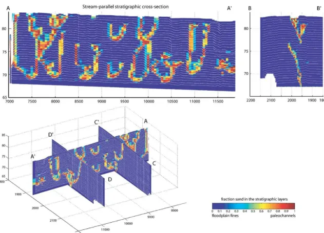
Figure 36. (A) Example of simulation of CHILD meander module. (B) Computational dynamic TIN-mesh used to self-update in result of lateral movement along main channel. (C) Static rectangular grid used for storage of subsurface stratigraphy. (D) Stratigraphic columns are stored as ordered lists of layers coupled to static grid elevations (Oualine, 1997). Layers are informed about age and grain size texture. (Image source: Clevis and al., 2006) ... 34 Figure 37. Stratigraphic cross-sections of simulation showing subsurface distribution of
paleo-channels (red, sand) and floodplain fines (blue, clay). A-A’: longitudinal cross-sections; B-B’: transversal cross-sections. Vertical axis represents 500-year time intervals (image source: Clevis and al., 2005) ... 35 Figure 38. Channel example in object-based model (Hauge and al., 2007) ... 36 Figure 39. Visual representation of streamline association cross-section (Pyrcz and Deutsch, 2005) .. 37 Figure 40. Event-based model simulation conditioned by areal trends (Pyrcz and Deutsch, 2005). (A) –
empty areal trend applied to (B) – non-conditional simulation. (C) – areal trend used in
conditioning and (D) – conditional simulation ... 38 Figure 41. Conditioning to well data in event-based model (Pyrcz and Deutsch, 2005) ... 39 Figure 42. Non-conditional (A, C) and conditional (B, D) event-based simulations (Pyrcz and Deutsch,
2005) ... 39 Figure 43. An example of well data. (a) – not interpreted resistivity log; (b) –large sandbodies from
large fluctuations of well logging (in yellow); (c) – well-interpreted data log, including smaller sand intervals (yellow), clay (green) and shale (blue). Data source: Wong et al., 2009 ... 41 Figure 44. Lithofacies classes definition tool for converting (a) discrete or (b) continous well log data
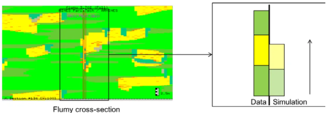
into Flumy facies (here: CL, PB, LV, etc.)... 42 Figure 45. Well data interpretation in Flumy ... 42 Figure 46. Flumy well view during conditioning simulations: left – Flumy cross-section, right –
schematic well illustration ... 43 Figure 47. The first case of specific data interpretation in Flumy: a small sand interval situated
between two clay bricks is interpreted as Crevasse Splay ... 45 Figure 48. The second case of specific data interpretation in Flumy: a small non-sandy interval
between two sandy facies is interpreted as Undefined facies ... 45 Figure 49. Example of Active Level and Active brick update ... 46 Figure 50. Main principles of migration adaptation in conditioning (R and r are distance parameters) 47
LIST OF FIGURES
xviii
Figure 55. The scheme of case Y (update AL algorithm) ... 51
Figure 56. The scheme of case Z (update AL algorithm) ... 52
Figure 57. The scheme of case ZT (update AL algorithm) ... 52
Figure 58. Scheme giving the elements for the computation of Von Mises distance ... 53
Figure 59. Example of points located at the same Von Mises distance from the well (the Ox axis represents the flow direction) ... 54
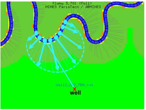
Figure 60. The Flumy channel 2D aerial view; the light blue points are the points with the corrected erodibility values, the straight lines are the velocity perturbation vectors The well (red cross) is linked to the nearest channel point according to the Von Mises distance. ... 55
Figure 61. “Repulsion” radius during the OB/WL data facies honoring ... 56
Figure 62. “Repulsion” and “attraction” radius during the LV/CSI/CSII/CCh data facies honoring ... 56
Figure 63. “Attraction” during the PB/CL/SP/MP data facies honoring ... 57
Figure 64. The avoidh scheme (migration adaptation) ... 58
Figure 65. The gap_up scheme (migration adaptation) ... 58
Figure 66. The above_al scheme (migration adaptation) ... 59
Figure 67. “Pseudo” topography during the OB/WL data facies honoring (3D Flumy view) ... 61
Figure 68. “Pseudo” topography during the LV/CSI/CSII/CCh data facies honoring (3D Flumy view) ... 61
Figure 69. The avoidh scheme (avulsions adaptation) ... 62
Figure 70. “Pseudo” topography during the PB/CL/CP/MP data facies honoring (3D Flumy view) ... 63
Figure 71. The gap_up scheme (avulsions adaptation) ... 63
Figure 72. The above_al scheme (avulsions adaptation) ... 64
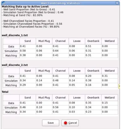
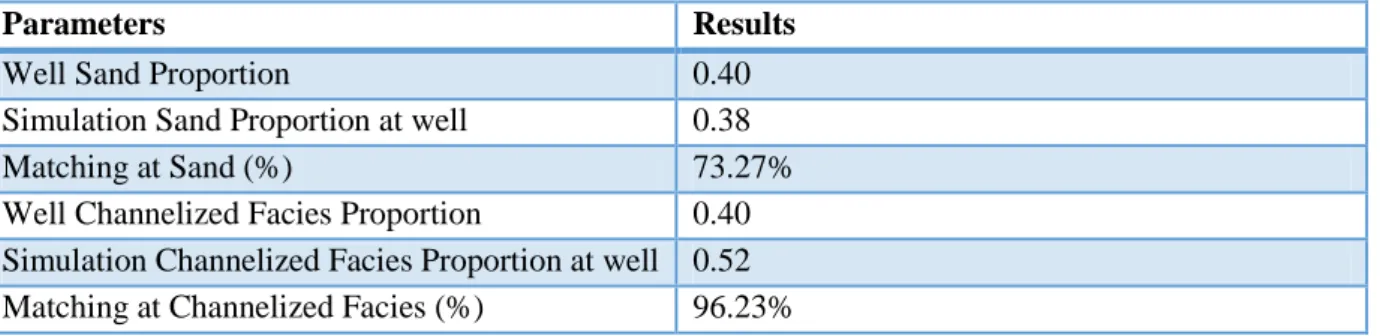
Figure 73. Matching between the well data and simulation results ... 67
Figure 74. Well conditioning statistics for each wells and for all wells combined ... 68
Figure 75. Example of cross-section comparison of non-conditional and conditional simulations ... 68
Figure 76. Sand Proportion Maps of non-conditional (left) and conditional by two wells (right) simulations, with the corresponding N_G ... 69
Figure 77. Non-Channelized facies well, with rich sand proportion: transversal cross-section containing well (left) and well reproduction (right) ... 71
Figure 78. Non-Channelized facies well, result of test with extremely ribbon sandbodies; transversal cross-section containing well (left) and well reproduction (right) ... 72
LIST OF FIGURES
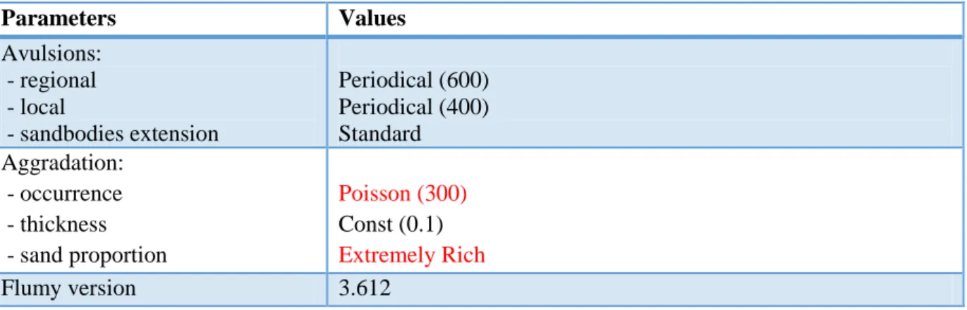
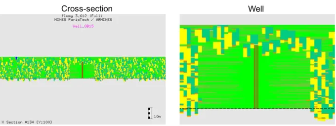
Figure 79. Channelized well reproduction, results of first (left) and second (right) tests with default parameters, Flumy version 3.612 ... 74 Figure 80. Channelized facies well, result of test with default parameters: transversal cross-section
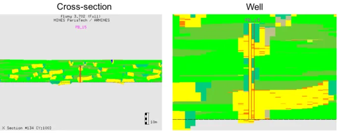
containing well (left) and well reproduction (right), Flumy version 3.702 ... 75 Figure 81. Channelized facies well, result of a test with small sand proportion: transversal
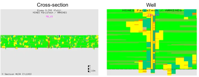
cross-section containing well (left) and well reproduction (right), Flumy version 3.702 ... 76 Figure 82. Channelized facies well, result of a ribbon sandbodies: transversal cross-section containing
well (left) and well reproduction (right), Flumy version 3.702 ... 77 Figure 83. Three-facies well reproduction, result of a test with default parameters, Flumy version
3.702 ... 79 Figure 84. Three-facies well reproduction, result of a test with high sand proportion, Flumy version
3.702 ... 81 Figure 85. Three-facies well reproduction, result of a test with sheet type sandbodies, Flumy version
3.702 ... 83 Figure 86. Conditions of four synthetic wells test, Flumy version 3.702 ... 85 Figure 87. Four synthetic wells reproduction, Flumy version 3.702 ... 86 Figure 88. Four synthetic wells test, comparison of cross-valley (a1-a2) and along flow (b1-b2)
sections of non-conditional and conditional simulations; Flumy version 3.702 ... 87 Figure 89. Conditional simulations with four extracted wells, Flumy version 3.702 ... 88 Figure 90. Four extracted wells reproduction, Flumy version 3.702 ... 89 Figure 91. Four synthetic wells test, comparison of cross-valley (a1-a2) and along flow (b1-b2) of
non-conditional and non-conditional simulations, Flumy version 3.702 ... 90 Figure 92. Sand Proportion Maps comparison, 2 wells test, non-conditional (left) and conditional
(right) simulations with resulting N_G, Flumy version 4.005 ... 93 Figure 93. Sand Proportion Maps comparison, 2 wells test, flow direction N-NW, with resulting N_G
... 93 Figure 94. Sand Proportion Maps comparison, 8 wells test, with resulting N_G ... 95 Figure 95. Sand Proportion Maps comparison, 7 wells aligned perpendicularly to the flow direction,
LIST OF FIGURES
xx Figure 99. Second case of new dynamic well interpretation ... 101 Figure 100. Case A1 in new Update AL algorithm ... 103 Figure 101. Case A2a in new Update AL algorithm ... 103 Figure 102. Case A2b in new Update AL algorithm ... 104 Figure 103. Case A3 in new Update AL algorithm ... 104 Figure 104. Case A4 in new Update AL algorithm ... 105 Figure 105. Case B1 in new Update AL algorithm ... 106 Figure 106. Case B2 in new Update AL algorithm ... 106 Figure 107. Case C in new Update AL algorithm ... 107 Figure 108. Case D in new Update AL algorithm ... 107 Figure 109. Case E in new Update AL algorithm ... 108 Figure 110. Case F1 in new Update AL algorithm... 109 Figure 111. Case F2 in new Update AL algorithm... 109 Figure 112. Case G0 in new Update AL algorithm ... 110 Figure 113. Case G1 in new Update AL algorithm ... 111 Figure 114. Case G2 in new Update AL algorithm ... 111 Figure 115. Case G3 in new Update AL algorithm ... 112 Figure 116. Case H1 in new Update AL algorithm ... 113 Figure 117. Case H2 in new Update AL algorithm ... 114 Figure 118. Case H3 in new Update AL algorithm ... 114 Figure 119. Sand Proportion Maps comparison, non-conditional simulation vers. 4.005 (left) and.
5.600 (right) with resulting N_G (flow to the north) ... 118 Figure 120. Sand Proportion Maps comparison, 15 extracted wells conditional simulation vers. 4.005
(left) and. 5.600 with old conditioning algorithm (right) with resulting N_G (flow to the North) ... 118 Figure 121. Three-facies well reproduction, default parameters, comparison of Flumy versions 3.702
(left) and 5.600 (right) ... 120 Figure 122. Three-facies well reproduction, small N_G, comparison of Flumy versions 3.702 (left) and 5.600 (right) ... 122 Figure 123. Three-facies well reproduction, large N_G, comparison of Flumy versions 3.702 (left) and 5.600 (right) ... 123
LIST OF FIGURES
Figure 124. Three-facies well reproduction, large avulsions period, comparison of Flumy versions 3.702 (left) and 5.600 (right) ... 124 Figure 125. Conditions of four synthetic wells test, Flumy version 5.600 ... 126 Figure 126. Four synthetic wells reproduction, Flumy version 5.600 ... 127 Figure 127. Four synthetic wells test, comparison of simulation cross-sections: non-conditional
simulation, vers. 3.702 (a1-a2); conditional simulation, vers. 3.702 (b1-b2); conditional
simulation, vers. 5.600 (c1-c2) ... 128 Figure 128. Conditions of four extracted wells test, Flumy version 5.600 ... 129 Figure 129. Four extracted wells reproduction, Flumy version 5.600 ... 130 Figure 130. Four extracted wells test, comparison of simulation cross-sections: non-conditional
simulation, vers. 3.702 (a1-a2); conditional simulation, vers. 3.702 (b1-b2); conditional
simulation, vers. 5.600 (c1-c2) ... 131 Figure 131. Sand Proportion Maps comparison, 2 wells test, Flumy vers. 4.005 (left) and Flumy vers.
5.600 (right) with resulting N_G ... 134 Figure 132. Sand Proportion Maps comparison, 8 wells test, Flumy vers. 4.005 (left) and Flumy vers.
5.600 (right) with resulting N_G ... 135 Figure 133. Sand Proportion Maps comparison, 7 wells aligned perpendicularly to the flow direction,
Flumy vers. 4.005 (left) and Flumy vers. 5.600 (right) with resulting N_G ... 136 Figure 134. Sand Proportion Maps comparison, 15 wells aligned perpendicularly to the flow direction, Flumy vers. 4.005 (left) and Flumy vers. 5.600 (right) with resulting N_G ... 138 Figure 135. Comparison of horizontal slices of two simulations: conditional by 15 aligned wells,
Flumy vers. 4.005 (left) and conditional by 15 aligned wells, Flumy vers. 5.600 (right). Z = 40m ... 139 Figure 136. Illustration of remaining problem, test of 15 wells aligned perpendicularly to the flow
direction: wells vertical cross-section contains less sand than the whole simulation ... 140 Figure 137. Comparison of Sand Proportion Matrices (above) and Simulation Proportion Matrices
(below), 15 wells aligned perpendicularly to the flow direction. From left to right: original test, vers. 5.600; test without migration repulsion for OB/LV reproduction, vers. 5.600; test without migration repulsion at all, vers. 5.600 ... 141 Figure 138. Comparison of vertical model cross-sections before the wells, containing the wells and
LIST OF FIGURES
xxii Figure 141. Example of (a) a dendrogram and (b) its graph of cluster dissimilarities using the Ward+
linkage criterion ... 155 Figure 142. Loranca basin: (a) location of the study area in the Tortola fan and (b) location of the
measured sections along the Rio Mayor valley sides with (c) an illustration of the architecture of isolated and amalgamated sand bodies ... 156 Figure 143. Location of wells for (a) the first synthetic case (20 wells), and (b) the second synthetic
case (8 wells) ... 158 Figure 144. First synthetic test with 3 contrasted units. (a) Reference VPC, red solid lines represent
initial units limits. (b) VPC of 20 extracted wells. (c) Cluster dissimilarities graph. (d) The last three clusters proposed by our method. ... 159 Figure 145. Second synthetic test with 5 less contrasted units. (a) Reference VPC, red solid lines
represent initial units limits. (b) VPC of 8 extracted wells. (c) Cluster dissimilarities graph. (d) The last five clusters proposed by our method ... 161 Figure 146. Application to a real dataset: Loranca basin. (a) 5 sections out of the 8 available, red solid
lines represent units limits proposed by geologists. (b) VPC of the 8 Loranca wells. (c) Cluster dissimilarities graph. (d) The last three clusters proposed by our method ... 163
LIST OF TABLES
List of tables
Table 1. Eleven Flumy lithofacies deposited during fluvial simulations ... 13 Table 2. Flumy lithofacies sorted in increasing grain size order ... 13 Table 3. List of 11 main Flumy simulation parameters ... 18 Table 4. Relation between the two lithofacies classifications in Flumy ... 44 Table 5. General Flumy simulation parameters for one-facies and multi-facies wells tests ... 69 Table 6. Flumy simulation parameters, test of Non-Channelized facies well, large sand proportion ... 70 Table 7. Flumy simulation parameters, test of Non-Channelized well, extremely ribbon sandbodies . 72 Table 8. Flumy simulation parameters, test of sand well, default parameters, Flumy version 3.612 ... 73 Table 9. Flumy simulation parameters, test of sand well, small sand proportion ... 76 Table 10. Flumy simulation parameters, test of sand well, ribbon sandbodies ... 77 Table 11. Flumy simulation parameters, test of three-facies well, default parameters, Flumy vers.
3.702 ... 79 Table 12. Resulting conditioning statistics, three-facies well, default simulation parameters, Flumy
version 3.702 ... 79 Table 13. Flumy simulation parameters, test of three-facies well, high sand proportion, Flumy vers.
3.702 ... 81 Table 14. Resulting conditioning statistics, three-facies well, large N_G, Flumy version 3.702 ... 81 Table 15. Flumy simulation parameters, test of three-facies well, sheet type sandbodies, Flumy vers.
3.702 ... 83 Table 16. Resulting conditioning statistics, three-facies well, large avulsions period, Flumy version
3.702 ... 83 Table 17. Simulation parameters of four synthetic wells test, Flumy version 3.702... 85 Table 18. Resulting conditioning statistics, four synthetic wells test, Flumy version 3.702 ... 86 Table 19. Simulation parameters of four extracted wells test, Flumy version 3.702 ... 88
LIST OF TABLES
xxvi Table 23. Resulting conditioning statistics, 2 extracted wells test, flow direction N-NW, Flumy version 4.005 ... 94 Table 24. Resulting conditioning statistics, 8 extracted wells test, Flumy version 4.005 ... 95 Table 25. Resulting conditioning statistics, 7 wells aligned perpendicularly to the flow direction,
Flumy version 4.005 ... 97 Table 26. Resulting conditioning statistics, 15 wells aligned perpendicularly to the flow direction,
Flumy version 4.005 ... 98 Table 27. Resulting conditioning statistics, 15 extracted wells test, Flumy versions 3.702 and 5.600
with old conditioning algorithm ... 119 Table 28. Flumy simulation parameters, test of three-facies well, default parameters, Flumy vers.
3.702 and 5.600 ... 120 Table 29. Resulting conditioning statistics, three-facies well, default parameters, Flumy versions 3.702 and 5.600 ... 120 Table 30. Flumy simulation parameters, test of three-facies well, small N_G, Flumy vers. 3.702 and
5.600 ... 121 Table 31. Resulting conditioning statistics, three-facies well, small N_G, Flumy versions 3.702 and
5.600 ... 122 Table 32. Flumy simulation parameters, test of three-facies well, large N_G, Flumy vers. 3.702 and
5.600 ... 123 Table 33. Resulting conditioning statistics, three-facies well, large N_G, Flumy versions 3.702 and
5.600 ... 123 Table 34. Flumy simulation parameters, test of three-facies well, large avulsions period, Flumy vers.
3.702 and 5.600 ... 124 Table 35. Resulting conditioning statistics, three-facies well, large avulsions period, Flumy versions
3.702 and 5.600 ... 125 Table 36. Simulation parameters of four synthetic wells test, Flumy versions 3.702 and 5.600 ... 126 Table 37. Resulting conditioning statistics, four synthetic wells test, Flumy versions 3.702 and 5.600
... 127 Table 38. Simulation parameters of four extracted wells test, Flumy versions 3.702 and 5.600 ... 129 Table 39. Resulting conditioning statistics, four extracted wells test, Flumy versions 3.702 and 5.600
... 130 Table 40. General simulation parameters for the tests of spatial sand distribution, Flumy versions
4.005 and 5.600 ... 133 Table 41. Resulting conditioning statistics, 2 extracted wells test, Flumy versions 4.005 and 5.600 . 134 Table 42. Resulting conditioning statistics, 8 extracted wells test, Flumy versions 4.005 and 5.600 . 135
LIST OF TABLES
Table 43. Resulting conditioning statistics, 7 wells aligned perpendicularly to the flow direction, Flumy versions 4.005 and 5.600 ... 137 Table 44. Resulting conditioning statistics, 15 wells aligned perpendicularly to the flow direction,
Flumy versions 4.005 and 5.600 ... 138 Table 45. Resulting conditioning statistics, 15 wells aligned perpendicularly to the flow direction,
Flumy versions 5.600, 5.600 without migration repulsion for OB/LV reproduction and 5.600 without migration repulsion at all ... 143
INTRODUCTION
Introduction
The need of models for heterogeneous reservoirs has stimulated the development of stochastic models that are relatively flexible and easy to condition: geostatistical Plurigaussian models (Galli and al., 1994; Le Loc’h and al., 1994; Armstrong, 2011), MPS simulations (Mariethoz and Caers, 2015), Boolean models (Lantuejoul, 2002; Chilès and Delfiner, 2012). However, the geometry and arrangement of sedimentary bodies reproduced by all these models may lack realism. Another solution to produce realistic reservoir models is to combine a stochastic and a process-based approach, providing that the geological processes are well enough known. The increasing performance of computer modeling techniques now allows simulating such process-based, or forward, models relatively easily.
Flumy is a forward model developed at MINES ParisTech, Geosciences research center, for meandering channelized systems. Initially dedicated to fluvial reservoirs (Lopez, 2003; Lopez and al., 2008), it is currently extended to turbiditic ones (Lemay et al., 2016). Simulations are performed based on channel migration, aggradation processes such as overbank floods and avulsion processes. Combination of these three different processes produces realistic and contrasted three dimensional architectures of meandering fluvial sequences.
Flumy simulations need a set of entry parameters. In order to create more realistic simulation, these parameters should be coherent with data (e.g., the wells). The determination of consistent simulation parameters has been a large subject in the development of Flumy model. In particular, if a modeled reservoir shows various stratigraphic units, the simulation parameters should be determined for each unit.
Soft and hard conditioning are proposed to the user: they are based on seismic and well input data, respectively. We will focus here on the well conditioning. The conditioning issue is a challenge for the process-based models because it requires not only to reproduce the known data at the well locations, but also to preserve at the same time the realism of the modeled sedimentary processes. In Flumy, the conditioning algorithm is a straightforward procedure (no trial/error, deposits at wells are to be reproduced during the simulation). It is based on the adaptation of the main fluvial processes (migration, aggradation and avulsion) during simulation for the lithofacies deposition required at the well location. This adaptation allows honoring the data, although not at 100%, but is also responsible for artifacts or distortions of bodies, which may alter the realism.
The first main objective of this thesis is to analyze and reduce the undesirable impact of the well conditioning by developing solutions to improve the conditioning procedures.
As said above, the parameters may change from one sedimentary unit to another one. The distinction of different units is a previous step in the modeling of reservoirs. However, it is not always straightforward. Thus, a second objective of this thesis is to propose an automatic way to assist the
INTRODUCTION
2 conditioning in Flumy. The main principles of conditioning are presented, with a further detailed description of initial conditioning techniques.
- the third chapter concerns the evaluation of initial conditioning procedures in Flumy. Two aspects are tested and illustrated: well data exact reproduction and sand spatial distribution in conditional simulations. Then, new algorithms are proposed to improve the conditioning in terms of a more uniform sand distribution over the domain and a better sand matching at well while respecting the lithofacies deposition characteristic for non-conditional simulations. At last, the new results are presented and discussed.
- the fourth chapter deals with a crucial point in reservoir modeling, the determination of the stratigraphic units from the well data. A new method based on geostatistical hierarchical clustering applied to the global well vertical sand proportion curve is presented and illustrated with some synthetic cases and a field case study.
CHAPTER 1
1 Flumy model for meandering fluvial systems
Résumé français : Ce chapitre introduit le modèle Flumy pour les systèmes fluviatiles méandriformes. Il commence par une description des principaux processus et dépôts liés aux systèmes méandriformes fluviaux, basée sur des exemples actuels et fossiles. Il présente ensuite la manière dont ces processus et dépôts sont simulés par Flumy. Il décrit enfin un outil, le Nexus (Non-Expert User Calculator), permettant le calcul automatique des paramètres du modèle à partir de trois d'entre eux.
In this chapter, we present a brief description of the main processes and depositional elements of the meandering fluvial systems based on modern and fossil examples. Then we present how these processes and associated depositional elements are simulated by Flumy. The automatic inference of the main simulation parameters by the Non-Expert User Calculator (Nexus) is presented at last.
1.1
Meandering Fluvial Systems
1.1.1 Modern systems
Modern meandering systems are dynamic fluvial systems (Figure 1, a). They are generally associated with sandy-clay loads, although there exist meandering systems with gravel and/or pebbles. The meandering channels are characterized by high migration potential, which results in the construction of sandy deposits on the inner banks of the meander loops – the meander point bars. These bars have lenticular to sigmoidal form and migrate transversely to the flow (Figure 1, c-d).
CHAPTER 1
6
1.1.1.1 Meandering channel geometry
In modern hydraulic studies, the channel geometry is defined by the bankfull geometry that corresponds to the water elevation before an overbank flood (Leopold and Wolman, 1957; Bridge, 2003). This channel bankfull geometry is characterized by the channel bankfull width and the mean bankfull depth:
• The bankfull width corresponds to the channel width at the bankfull stage elevation, defined at the top of the point bar (Williams, 1978; Sweet and Geratz, 2003). The channel bankfull width is relatively stable along the channel path.
• The mean bankfull depth is obtained by dividing the channel cross section area by the bankfull width.
The maximum channel depth (difference in elevation between the deepest and the highest one in the surveyed section) is dependent of the channel curvature, the occurrence of riffles and pools. It is maximum at the apex of the bend and corresponds to 1.7 the mean bankfull depth (Bridge, 2003).
(a) (b)
Figure 2. (a) Cross-section in a straight reach mean bankfull depth; (b) cross-section at the bend apex max bankfull depth (From Held, 2011).
This bankfull geometry proved to show good relationship with the channel forming discharge in fluvial systems in humid climates (Bridge, 2003 and references therein). It is used in the restoration of man-managed meandering fluvial system towards natural courses or for paleohydrologic studies (Williams, 1986). In Flumy, the classical power relationship between channel geometry and discharge (Leopold et al., 1964) are used for the channel width/maximum depth ratio. This ratio is taken as 10, based on a power coefficient close to 1:
𝑤 = 10 ∗ ℎ1,
where w – the channel width, h – the channel maximum depth.
1.1.1.2 Evolution of the meander loops
During migration, the meander loops extend, resulting in a narrowing of the distance between the upstream and downstream channel reaches of the meander bend that can result in a neck or chute cutoff when they are very close (Figure 3, a-b). Thus, the course of the river is modified and eventually an abandoned meander loop is created (oxbow) which creates a more or less efficient junction between the floodplain and the channel. These abandoned meanders are then progressively
(a)
CHAPTER 1
filled up by the fine grained sediments transported during the successive floods and form sand and clay plugs. In relatively humid climates, the floodplain is never completely drained, the depressions left by these abandoned meanders are occupied by marshy lake systems (oxbow lake) and may be filled with peat.
With time, the channel migrates across the floodplain, building a channel belt. The channel belt corresponds to the area where the channel paths have been mainly confined (Figure 3, c-d). Many oxbow deposits are preserved on the edges of the channel belt. Their fine grained filling limits migration further away in the floodplain.
(a) (b)
(c) (d)
Figure 3. Illustration of a meander loop by neck cutoff (a) and chute cutoff (b) (Dieras, 2013); (c) map of the Mississippi channel belt built over some ten thousand years (Fisk, 1944); (d) satellite photo of the Jutaï River (Amazon, North Brazil) extracted from Google Earth. This picture shows the meandering belt formed by a high
sinuosity river, within which meander intersections also cause the formation of lakes and dead arms.
1.1.1.3 Overbank flow sediments
CHAPTER 1
8
(a) (b)
Figure 4. (a) Scheme of overflow sediments formation; (b) the Red River during the 1997 flood, viewed southwards from near St. Norbert, Manitoba (Canada). Courtesy Geological Survey of Canada (up), and Missouri River flood
(2018 Scripps Media, Inc.) (below)
This results in a transition between the channel and the floodplain marked by a system of levees, elongated sandy to silty bodies that lie along the channel (Figure 4, b). Although present on both banks, they are more developed on the outer bank. Thus, the levees are formed during flood episodes (overbank) and therefore have a low potential for preservation because they can be eroded during channel migration (Reading, 1978; Brierley et al., 1997). The sedimentation rates of the floodplain are low and decrease with the distance to the channel due to the loss of velocity of the flow which is no longer channelized. It results in the deposition of the fine grained sediments away from the channel, leaving thin layers of silty to shaly alluvium.
The floodplain lowlands are often occupied by wetlands, swamps or lakes depending on the water table level. Areas of higher elevation are the site of pedogenesis in relation with the type of vegetation cover and climate.
1.1.1.4 Levee breaches
The violent floods sometimes cause a sudden rupture of the banks (a levee breach) which can go up to the abandonment of the initial channel path to a new one, resulting in a complete avulsion of the channel. In less severe cases, the levee breach may cause diversion of part of the flow into the floodplain, with deposition of crevasse splays (Figure 5). The levee breach may heal, and the channel keeps its initial path. The water flowing through the levee breach is loaded with coarser sedimentary load than the overbank flow, resulting in crevasse splays composed of relatively coarse sandy to silty material.
CHAPTER 1
(a) (b)
Figure 5. (a) Levee breach along the Mississippi River (source: http://www.20min.ch/ro/news/monde/story/14925437); (b) Crevasse splay, Columbia River, Canada (source: http://www.seddepseq.co.uk/)
1.1.2 Fossil systems
In fossil systems, meandering channel elements can be easily identified based on the geometry of the sedimentary beds, their mineralogical composition and the grain size. Here is a list of principal elements characteristics, illustrated by photos from the Miocene Loranca fluvial deposits (Spain, La Mancha):
• sandy point bar deposits are represented by low angle inclined sandy sets that correspond to migration periods (Figure 6)
Figure 6. Point bar of around 3m height, showing the lateral extension of 18-20m
CHAPTER 1
10 Figure 8. Paleosol
• crevasse splay deposits show very often an erosive contact with the underlying deposits, and are always coarser than the levee or overbank deposits (Figure 7)
• oxbow lakes are filled by clay rich deposits overlaid by a limestone bed (Figure 9)
Figure 9. Oxbow lake with orange clayey deposits and white facies limestone bed. The person is standing on the toe of the last point bar set before the loop abandonment
• low land deposits, depending on the climate, can be represented by organic rich deposits or carbonate-rich ones.
CHAPTER 1
The preservation of these architectural elements in fossil systems depends on the balance between the aggradation and migration rates. Low aggradation rates result in cannibalization of the point bar deposits, numerous mud plugs and well developed soils in the stable floodplain. On the other hand, high aggradation rates favor preservation of the various facies associated to the fluvial meandering systems (Figure 11).
Figure 11. Isolated sandbodies in the alluvium deposits during a period of high aggradation rate; on top – amalgamated sandbodies during a period of low aggradation rate.
The following scheme (Figure 12) contains a summary of main depositional facies presented in modern and fossil meandering systems, illustrated by the Miocene deposits photos of the Loranca basin (Spain).
CHAPTER 1
12
1.2
Flumy model
Starting from the 1950s, meandering fluvial systems became an object of active field and theoretical studies (Leopold and Wolman, 1957, 1960). These observations, combined with laboratory experiments (Friedkin, 1945), allows now predicting the evolution of meandering rivers quite well (Bridge, 2003; Castro and Jackson, 2001; Mulvihill and Baldigo, 2007). Several generations of models have been developed, that relate the migration rate of river centerline to the integrated effect of velocity asymmetry in meander bends (Howard and Knutson, 1984; Ikeda et al., 1981; Ikeda and Parker, 1989; Johannesson and Parker, 2013; Perucca et al., 2007; Sun et al., 2001). All these lead to 2D reproduction of the long-time behavior of meandering channels, including the dynamic of channel flow and the resulting deposition patterns.
The Flumy software is a modeling tool, both process-based and stochastic, which aims to provide accurate and realistic 3D representations of the simulated sandbodies and their associated deposits at the scale of the reservoir (Lopez, 2003; Lopez et al., 2001, 2008; Lemay et al., 2016).
The model construction is based on three main processes:
1) the channel migration with the deposition of sandy point bars in the interior part of meander loops, and sand and mud plugs in abandoned channels;
2) the aggradation process caused by overbank floods, with the construction of silty levees and fine-grained alluvium deposition on the floodplain;
3) the channel wandering thanks to the avulsions – results of the levee breaches, which possibly lead to the creation of new channel paths.
The combination of these three processes enables simulating the depositional facies mentioned above; resulting simulation is illustrated in Figure 13 and explained in details in the following subchapters.
CHAPTER 1
During simulation deposits are saved at each node of the 2D grid corresponding to the simulation domain. Information regarding the simulated deposits comprises: X, Y, Z coordinates and thickness; lithofacies, grain size and age (Figure 14):
Figure 14. Different color scales in Flumy
The next Table 1 contains the information about the lithofacies types deposited during different processes (as well as their visualization colors):
Table 1. Eleven Flumy lithofacies deposited during fluvial simulations
The Table 2 shows, sorted in increasing grain size order, the relation between the 11 possible fluvial lithofacies and their grain size. In the rest of this manuscript, Flumy lithofacies could be named “facies” only.
CHAPTER 1
14
1.2.1 Migration
The model is based on the evolution of the channel centerline in time and on the deposition of the associated sedimentary bodies. The 2D river hydraulic equations proposed by Ikeda and collaborators (Ikeda et al., 1981) proved to produce realistic shapes (Lopez, 2003, PhD thesis; Lopez et al., IAS 2008).
Linearization of the main hydraulic equations in the 1980s made possible to propose theoretical equations that replaced the empiric formulae deduced from observations (Ikeda et al., 1981, Johannesson and Parker 1989b, c; Sun et al, 2001). The main hypothesis underlying these models of the geometrical evolution in space and time of meandering rivers is a linear relationship between the lateral migration of the channel and the flow velocity close to the river bank. These linear theories proved to give stable algorithms to model long-term evolution of meandering rivers.
The channel centerline is discretized into several channel points with Cartesian coordinates. The flow velocity U depends from the global valley slope I and the mean channel wavelength λ. It is considered constant along the channel. At every channel point, the following properties are calculated: the curvature k, the Cartesian distance from the previous upstream point ∆s, the normal vector n and the
velocity perturbation U’ collinear to the normal vector.
In Flumy, the classical model created by Ikeda et al. (1981) is used, with an adaptation made by Johannesson and Parker (1989) and Lopez (2003):
Figure 15. Channel centerline scheme (Parker and al., 2011)
Erosion and migration at the outer bank linearly related to the velocity perturbation (𝑈𝑏′) are presented as following:
𝑚𝚤𝑔
��������⃗ = 𝑛�⃗ 𝑈𝑏′ 𝐸,
where E is the bank erodibility coefficient. The smaller this coefficient is, the lower bank erodibility, the slower migration of the meander.
So, for each channel point, the local velocity perturbation 𝑈𝑏𝑖+1′ is calculated according to: 𝑈𝑏𝑖+1′ = 𝑈𝑏𝑖′ �1 − 2 ∆𝑠𝑖 𝐶𝐻 � + 𝑘𝐹 𝑖+1𝐵𝑈 − 𝑘𝑖𝐵𝑈 �1 + ∆𝑠𝑖𝐶𝐻 �𝑓 𝑈
2
𝑔𝐻 + 𝐴𝑎𝑓𝑓+ 𝐴𝑠𝑒𝑐− 1��, where 𝑈𝑏𝑖+1′ – local velocity perturbation (m/s);
𝑈𝑏𝑖′ – upstream velocity perturbation (m/s);
∆𝑠𝑖 – distance between upstream node i and local node i+1 (m);
CHAPTER 1
𝑘𝑖 – upstream curvature (const);
B – bankfull half-width of channel (m); H – bankfull mean depth (m);
U – mean velocity longitudinal component (m/s); g – gravitational acceleration (m/s2);
𝐶𝑓 – friction coefficient (const);
𝐴𝑎𝑓𝑓 – vortex coefficient (const);
𝐴𝑠𝑒𝑐 – secondary current coefficient.
These equations are used to simulate the channel centerline migration, accompanied by deposition of sand point bars, and mud plugs in the oxbow lakes created by cutoffs (Lopez, 2003; Lopez et al., 2004 EAGE).
Based on these equations, the meander loops develop a stable pattern from an initial straight centerline with small perturbations. Migration is performed at each iteration (1 year for fluvial systems). Amplitude of the migration is driven by the curvature of the centerline and the erodibility of the substratum. By default, the erodibility is constant over the domain. The erodibility can be defined locally, thus favoring migration in the areas of higher erodibility. After several iterations, some cutoffs occur and meander loops are abandoned. Figure 16 shows the meanders development:
Figure 16. An illustration of meanders development in Flumy
Channel cross-section (Figure 17): geometry of each depositional unit depends on the local curvature of the channel.
Figure 17. Flumy channel cross-section example. In blue – the channel with the water inside, from red to yellow color – deposited sandy Point Bars from the old to new deposits
Principal parameters associated to the migration are: erodibility coefficient E, channel bankfull width
w, channel bankfull mean depth H global valley slope I (along flow direction) and mean wavelength
CHAPTER 1
16 Figure 18. Flumy valley cross-section scheme (vertical scale exaggeration)
Figure 19. Overbank Flood in Flumy (cross-section and 3D view)
In the fluvial systems, peat (or any wetland deposits) may be deposited in the lowlands as illustrated on Figure 20.
Figure 20. Flumy cross-section with wetland depositions on the floodplain
Principal characterization parameters for aggradation are: overbank flood thickness iob (constant, or
defined by Uniform/Normal/Log-normal distribution)and period Tob (constant or defined by Poisson
distribution), thickness exponential decrease λob, and levee width LLV.
1.2.3 Levee breaches and avulsions
From time to time, a levee breach may occur, preferentially where the velocity perturbation is locally maximal. This results either in a chute cutoff, or in the deposition of a crevasse splay possibly followed by an avulsion (the new channel finds a new path downstream using a stochastic steepest path algorithm) (Figure 21).
There exist two types of avulsions in the model: local, when a new path is tossed from a levee breach point within the domain, and regional, in order to simulate a levee breach upstream of the domain (Figure 22). The regional avulsions, ensure a uniform spatial distribution of the channel paths over the modeled domain through time.
CHAPTER 1
Figure 21. A local (left) and a regional (right) avulsion in Flumy, 3D view Note:
Figure 22
after a successful regional avulsion, the channel may lie outside the simulated domain, and reenter the domain from the lateral sides by migration or avulsions ( ):
Figure 22. New channel path examples (resulting from a regional avulsions) Principal characterization parameters for avulsions are: local avulsion period T
LAV and regional
avulsion period T
CHAPTER 1
18
1.2.4 Conclusion
Flumy is a process-based and stochastic model for channelized fluvial meandering reservoirs. The simulations are performed forward. The output is a three-dimensional numerical blocks, informed with lithofacies, grain size and age for each deposition unit.
Time is discretized into iterations, or time steps. At every time step, migration is performed, with deposition of sandy point bars in outer part of meanders. When overbank flow occurs, fine grain material is deposited on the domain, with thickness and grain size decreasing exponentially from the channel. Avulsions, generated during levee breaches within the domain or upstream of the domain allow a uniform distribution of the sandy sediments over the domain thanks to new channel paths formation.
The model is finally ruled by eleven main parameters (Table 3).
Parameter Symbol Processes
Channel maximum depth Hmax (m)
Migration
Channel width w (m)
Mean wavelength λ (m)
Erodibility coefficient E (m/s)
Global slope along flow direction I (const) Overbank flood thickness iob (m)
Aggradation Overbank flood period Tob (number of iterations)
Thickness exponential decrease λob (m)
Levee width LLV (multiple of w)
Local avulsions period TLAV (number of iterations)
Avulsions Regional avulsions period TRAV (number of iterations)
Table 3. List of 11 main Flumy simulation parameters
These allow simulating contrasted reservoir architectures by just varying the migration, the aggradation and the avulsion parameters. Thanks to the stochastic aspect, multiple realizations of the model can also be produced using the same set of parameters. One of the Flumy objectives is the possibility to create blocks with various sandbodies distribution. Figure 23 illustrates the simulation results variability: Sixteen cross-sections of different models are sorted in function of two main characteristics: aggradation rate and avulsion period.
CHAPTER 1
Figure 23. Variability of Flumy results in function of aggradation rate and avulsions period (Flumy cross-section view of 16 different scenarios)
For an easy use of the software, a tool to deduce all main parameters from a reduced number of parameters has been developed and is presented in the next chapter.
CHAPTER 1
20
1.3
Flumy – Non-Expert User Calculator (Nexus)
It may be difficult for a non-expert Flumy user to determine all the simulation parameters. In order to simplify this task, a special tool is proposed: The Non-Expert User Calculator (Nexus). It is based on some heuristic formulas coming from the Boolean model (Rivoirard et al., 2008) applied to the sedimentary objects generated by Flumy. The Nexus only gives orders of magnitude for the main parameters. At last, the user can choose to adjust the proposed parameters.
The three key Nexus parameters are the following: • The Channel Maximum Depth (Hmax),
• The Required Net-to-Gross (N_G, or sand proportion). • The Sandbodies Extension Index (Isbx)
1.3.1 Key Nexus parameters
• Channel Maximum Depth
The channel maximum depth (Hmax in meters) corresponds to the channel maximum bankfull depth.
Due to the simplified parabolic shape of the channel cross-section in Flumy, the channel mean bankfull depth used by the migration process is calculated by dividing the maximum depth by 1.5. The channel maximum depth gives information related to the scale of the resulted reservoir.
• Sand Proportion
This key parameter is the desired sand proportion in the resulted simulation (N_G in percentage). It can be either given from well data, field sections or chosen by the user. Four Flumy lithofacies are considered as sand: Point Bar (PB), Channel Lag (CL), Sand Plug (SP) and Crevasse Splay I (CSI).
• Sandbody Extension Index
The Isbx refers to the horizontal Sandbody Extension Index (from 20 to 160, no-unit). It is a parameter
characterizing the lateral amplitude of the channel meanders (maximum distance from meander centerline to the line joining the two inflexion points delimiting the bend. It characterizes the type of sandbodies:
• Isbx from 20 to 80 corresponds to ribbon-type sandbodies;
• Isbx from 80 to 100 is for standard sandbodies; meander loops are well developed but not at
their maximum;
• Isbx > 100 is for sheet-type sandbodies; the largest amplitude is reached during neck cutoff.
The tests conducted with different Flumy scenarios show that the ratio between the mean sandbody extension (L, in m) and the wavelength (λ, in m) stabilizes after the occurrence of the first cutoff. So, small values of L/λ (0.2) correspond to the less developed ribbon-type sandbodies. Then, the channel curvature starts to increase, and the values of L/λ from 0.2 to 0.4 indicate a standard type sandbodies (until the first meander cutoff). The tests showed that the first cutoff corresponds to L/λ≈0.4, with a further stabilization of this relationship value, so starting from 0.4 the sheet sandbodies are modeled. The next scheme (Figure 24) illustrates the choice of Isbx value thresholds from the L/λ graph.
CHAPTER 1
Figure 24. Illustration of Isbx possible values and its influence on the simulation results (Flumy aerial 2D view)
1.3.2 Use of the Nexus
When applying the Nexus from the three key parameters, all other parameters are computed automatically. It should be mentioned that even after the determination of the parameters by the Nexus, the user keeps the access to all parameters and can change their proposed value. The Nexus can be considered as a tool that provides “a first guess” of the simulation parameters from the three key parameters.
The determination of the parameters by the Nexus is performed following these steps (Figure 25): - The first step calculates all scaled parameters (the channel geometry, the overbank flood
thickness and the erodibility coefficient) from Hmax. As a consequence, the grid parameters
(size, mesh) can be adjusted to have a good display of the channel (mesh size ≤ w/2).
- The second step defines the overbank flood period by combining channel geometry with the required N_G.
- The third step defines the local and regional avulsions periods using the Isbx parameter.
Apart from that, the Nexus permits to determine the forecasts resulting sand proportion and aggradation rate which are displayed during the simulation.
When running a Flumy simulation, some other channel and block model statistics are calculated and displayed like the mean topography or the current channel sinuosity.
CHAPTER 1
22 Figure 25. Schematic illustration of Non-Expert User Calculator
Combination of the Isbx and N_G key parameters for a given channel size offers the possibility to
generate reservoir simulations with contrasted sandbody geometries as illustrated on Figure 26. Here, only simulated sandbodies are presented in 3D model view (scorched view); three different N_G values (20%, 40% and 60%) are simulated with various sets of Isbx for a constant value of Hmax.