de
l’Université de recherche Paris Sciences et Lettres
PSL Research University
Préparée à
l’Université Paris-Dauphine
COMPOSITION DU JURY :Soutenue le
par
ecole Doctorale de Dauphine — ED 543
Spécialité
Dirigée par
N o u v e a u x m o d Ł l e s d e c h e m i n s m i n i m a u x p o u r l ’ e x t r a c t i o n d e s t r u c t u r e s t u b u l a i r e s e t l a s e g m e n t a t i o n ...
27-09-2016
Da CHEN
Laurent D. COHEN
University Paris Dauphine Laurent D. COHEN
Technion - Israel Institute of Technology Ron KIMMEL
Remco DUITS
Eindhoven University of Technology
G a b r i e l P E Y R University Paris Dauphine
Jean-Marie MIREBEAU
U n i v e r s i t Ø P a r i s - S u d
G r Ø g o i r e M A L A N D A I N INRIA Sophia Antipolis
Roberto ARDON
Philips Research Medisys
Michel PAQUES
Tubular Structure Extraction and
Image Segmentation
by
Da CHEN
Supervisor: Prof. Laurent D. Cohen
A thesis submitted for the degree of
Doctor of Philosophy
in the
CEREMADE, CNRS, UMR 7534
Universit´e Paris Dauphine, PSL Research University
My deepest gratitude naturally goes first to my supervisor Prof. Laurent D. Cohen, without whom this thesis would not be possible. I am extremely lucky to be his Ph. D student. His knowledge, enthusiasm, expertise and experience make me to enjoy the research work during the past four years.
I would like to express my heartfelt gratitude to Dr. Jean-Marie Mirebeau, who gave me exciting and constructive help that facilitates my entry into the field of numerical analysis. A substantial part of this work was initiated by a collaboration with Dr. Jean-Marie Mirebeau.
I would like to warmly thank all the members of my thesis committee. I would like to give my appreciation to Prof. Ron Kimmel and Prof. Remco Duits who kindly gave me some of their extremely valuable time to carefully read this manuscript and to write the reports. I am also very honoured by the presence of prof. Gr´egoire Malandain, Prof. Michel Paques, Prof. Gabriel Peyr´e, and Dr. Roberto Ardon in my defense as examiners. Particularly, I thank Prof. Michel Paques who gave some motivation for retinal vessel tree analysis at an early stage of this work.
I also would like to give my appreciation to Prof. Alfred M. Bruckstein for his fruitful discussion on my subject.
I would like to thank CEREMADE that funds me to join many international conferences (even including trips to China and America) in the past four years. I thank China ScholarShip Council for the financial support to finish this thesis. I thank the entire team of CEREMADE, University Paris Dauphine to provide me various help for my daily work. I am also very grateful to my colleagues Fang Yang, Qi-Chong Tian, Emmanuel Cohen for their fruitful discussion on my subject. I also would like to thank my Chinese friends Ke Wang, Hua Lu, Bang-Xian Han,
gave me great help to evaluate my models.
I have a special gratitude to all my family, especially to my parents. Thank you for the unconditional support during the past four years.
Finally, let me convey my sincerest gratitude to my wife Han Li for her concomi-tance all the time. Whatever the situation is, you always support and believe me. My true gratitude is beyond any words description. I believe that this thesis is one of the most precious efforts we have experienced.
In the fields of medical imaging and computer vision, segmentation plays a crucial role with the goal of separating the interesting components from one image or a sequence of image frames. It bridges the gaps between the low-level image pro-cessing and high level clinical and computer vision applications. These high level applications may include diagnosis, therapy planning, object detection and recog-nition and so on. Among the existing segmentation methods, minimal geodesics have important theoretical and practical advantages such as the global minimum of the geodesic energy and the well-established fast marching method for numer-ical solution. In this thesis, we focus on the Eikonal partial differential equation based geodesic methods to investigate accurate, fast and robust tubular structure extraction and image segmentation methods, by developing various local geodesic metrics for types of clinical and segmentation tasks.
This thesis aims to apply different geodesic metrics for the Eikonal partial dif-ferential equation framework to solve different image segmentation and boundary detection problems especially for tubularity segmentation and region-based ac-tive contours models, by making use of more information from the image feature and prior clinical knowledges. The designed geodesic metrics basically take ad-vantages of the geodesic orientation or anisotropy, the image feature consistency, the geodesic curvature and the geodesic asymmetry property to deal with vari-ous difficulties suffered by the classical minimal geodesic models and the active contours models. This thesis eventually presents the interpretation of classical image processing models: the Euler elastica model and the active contours mod-els by the framework of the Eikonal partial differential equation based minimal geodesics. Therefore, those classical models can share the advantages of the min-imal geodesics.
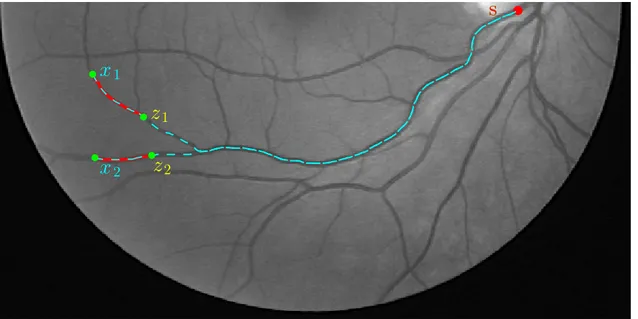
Upon the mathematical models developed in this thesis, we show the power of the minimal geodesics in the challenging clinical task of retinal blood vessels extraction including both the centreline positions and the corresponding vessel width values at these positions. Combining with the novel metrics investigated in this thesis, the minimal paths inspired solution to this task thus is able to benefit from the fast numerical solver such as the fast marching method, and easy user intervention, thus very practical and flexible. These models provide the possibilities to satisfy
Keywords: Minimal path, geodesic, Eikonal partial differential equation, im-age segmentation, tubular structure segmentation, active contours, Euler elastica curve, Riemannian meric, Finsler metric, curvature penalty, fast marching method.
Dans les domaines de l’imagerie m´edicale et de la vision par ordinateur, la seg-mentation joue un rˆole crucial dans le but d’extraire les composantes int´eressantes d’une image ou d’une s´equence d’images. Elle est `a l’interm´ediaire entre le traite-ment d’images de bas niveau et les applications cliniques et celles de la vision par ordinateur de haut niveau. Ces applications de haut niveau peuvent inclure le diag-nostic, la planification de la th´erapie, la d´etection et la reconnaissance d’objet, etc. Parmi les m´ethodes de segmentation existantes, les courbes g´eod´esiques minimales poss`edent des avantages th´eoriques et pratiques importants tels que le minimum global de l’´energie g´eod´esique et la m´ethode bien connue de Fast Marching pour obtenir une solution num´erique. Dans cette th`ese, nous nous concentrons sur les m´ethodes g´eod´esiques bas´ees sur l’´equation aux d´eriv´ees partielles, l’´equation Eikonale, afin d’´etudier des m´ethodes pr´ecises, rapides et robustes, pour l’extrac-tion de structures tubulaires et la segmental’extrac-tion d’image, en d´eveloppant diverses m´etriques g´eod´esiques locales pour des applications cliniques et la segmentation d’images en g´en´eral.
Cette th`ese vise `a appliquer diff´erentes m´etriques g´eod´esiques dans le cadre de l’´equation Eikonale, afin de r´esoudre diff´erents probl`emes de segmentation d’image et de d´etection de fronti`ere, en particulier pour la segmentation de structures tubu-laires et les mod`eles de contours actifs r´egion, en faisant usage de plus d’informa-tions issues des caract´eristiques d’image et de connaissances cliniques pr´ealables. Les m´etriques g´eod´esiques introduites tirent essentiellement leurs avantages de l’orientation g´eod´esique et de l’anisotropie, de la coh´erence des caract´eristiques de l’image, de la courbure g´eod´esique et de la propri´et´e g´eod´esique d’asym´etrie pour faire face aux diverses difficult´es pos´ees par les mod`eles classiques de g´eod´esiques minimales et les mod`eles de contours actifs. Enfin, cette th`ese pr´esente une in-terpr´etation des mod`eles classiques de traitement d’image: le mod`ele Elastica d’Euler et les contours actifs, par les g´eod´esiques minimales bas´ees sur l’´equation aux d´eriv´ees partielles Eikonale. Par cons´equent, ces mod`eles classiques peuvent tirer profit des avantages des g´eod´esiques minimales.
A propos des mod`eles math´ematiques d´evelopp´es dans cette th`ese, nous montrons la puissance des g´eod´esiques minimales pour l’extraction des vaisseaux de la r´etine, tˆache clinique souvent difficile `a r´ealiser, en indiquant `a la fois la ligne m´ediane
Cette th`ese contribue principalement `a l’´etude approfondie des diverses m´etriques g´eod´esiques et leurs applications en imagerie m´edicale et segmentation d’images. Des exp´eriences ont ´et´e r´ealis´ees sur des images m´edicales et des images naturelles pour montrer l’efficacit´e des contributions pr´esent´ees.
Mots-cl´es: Chemin minimal, g´eod´esique, ´equation aux d´eriv´ees partielles, ´equation Eikonale, segmentation d’images, segmentation de structure tubulaire, contours actifs, courbe Elastica d’Euler, m´etrique de Riemann, m´etrique de Finsler, p´enalit´e de courbure, m´ethode de Fast Marching.
English speakers are invited to go to Chapter 1 for the English version of this introduction.
La segmentation des images joue un rˆole essentiel dans le domaine du traitement d’images, liant le traitement d’images de bas niveau, comme le d´ebruitage d’im-ages, la restauration et l’am´elioration d’images et les taches de haut niveau pour des applications en imagerie m´edicale ainsi que la vision par ordinateur. L’ob-jectif fondamental de la segmentation d’images consiste `a obtenir une partition de l’image c’est `a dire une collection de r´egions, qui sont g´en´eralement disjointes les unes des autres. La segmentation d’images est encore un probl`eme difficile `a r´esoudre, puisque diff´erents types d’images n´ecessitent diff´erentes m´ethodes de segmentation.
Il existe un grand nombre de m´ethodes de segmentation, celle-ci ont ´et´e ´etudi´ees au cours des derni`eres d´ecennies. Parmi elles, la classe des m´ethodes de seuillage qui est largement utilis´ee est g´en´eralement consid´er´ee comme l’´etape de segmen-tation brute suivie de proc´edures de raffinement, grˆace `a la facilit´e de sa mise en oeuvre et `a une faible complexit´e. Ces m´ethodes utilisent l’information des niveaux de gris ou bien l’information en couleurs de chaque pixel ou groupe de pixels (comme un patch de l’image) et attribuent la mˆeme ´etiquette aux pixels ayant des propri´et´es similaires. Cependant, sans une r´egularisation des pixels, ces proc´ed´es de seuillage sont le plus souvent sensibles au bruit. En outre, ces m´ethodes de segmentation ne sont pas capables d’int´egrer des informations plus complexes et utiles, telles que la texture, la connaissance deforme pr´ealable et l’in-teraction de l’utilisateur. Pour pallier ce probl`eme, des m´ethodes de segmentation plus modernes ont ´et´e d´evelopp´ees, comme les mod`eles bas´es sur les graphes et les m´ethodes variationnelles de mod`eles d´eformables.
Des m´ethodes de segmentation bas´ees sur les graphes ont ´et´e propos`ees tels que le mod`ele de normalized cut propos´e par (Shi and Malik, 2000), la m´ethode de segmentation graph cut (Boykov and Funka-Lea, 2006) ainsi que la m´ethode de segmentation par marche al´eatoire (Grady, 2006). La formulation de ces mod`eles suppose que les images soient bas´ees sur le domaine discret consid´erant une image comme un graphe compos´e d’arˆetes et de noeuds. L’optimisation des ´energies
fronti`eres des r´egions de l’image peut ˆetre envisag´ee. Le terme de r´egularisation le plus populaire est la minimisation de la longueur Euclidienne des bords. R´ecemment, certaines de ces techniques mises en place par (El-Zehiry and Grady,2010; Schoen-emann et al.,2012) proposent de meilleurs r´esultats au niveau de la segmentation dans certains cas, comme pour les images dot´ees de structures `a la fois longues et fines.
Les mod`eles de contours actifs sont con¸cus pour minimiser une fonctionnelle d’´energie de la courbe dans le domaine continu sur la base des ´equations d’Euler-Lagrange et de principes variationnels. L’id´ee fondamentale du mod`ele des con-tours actifs (Kass et al., 1988) est de d´eformer la courbe ou ’snake’ convergeant vers les bords de l’objet tant par des forces internes que par des forces externes. La force interne peut assurer d’obtenir des contours actifs qui sont lisses, tandis que les forces externes, calcul´ees en fonction de donn´ees images, peut attirer les contours actifs vers les fronti`eres. Dans ce sens, diverses forces externes (Cohen, 1991; Cohen and Cohen, 1993; Xie and Mirmehdi, 2008; Xu and Prince, 1998) ont ´et´e propos´ees pour am´eliorer la performance du mod`ele des contours actifs. Les mod`eles des contours actifs g´eom´etriques (Caselles et al., 1993, 1997) sont bas´es sur le flux de mouvement par courbure Euclidienne. Dans leur formulation de base, les contours actifs sont repr´esent´es par l’ensemble de niveau z´ero d’une fonction (Osher and Sethian, 1988). Ces mod`eles g´eom´etriques sont en mesure de faire automatiquement face aux changements topologiques grˆace `a l’´evolution de la courbe bas´ee sur l’ensemble de niveau. Le principal inconv´enient de ces ´equations d’Euler-Lagrange, inspir´ees des mod`eles de contours actifs, est qu’elles tombent parfois dans des contours parasites provoqu´es par le bruit ou par les h´et´erog´en´eit´es d’intensit´e. Ces contours actifs ont ´egalement une energie non-convexe. Ainsi, il est difficile de trouver les minimums globaux des energies.
Un mod`ele de chemin minimal a ´et´e propos´ee par (Cohen and Kimmel,1997) afin de trouver le minimum global de l’´energie g´eod´esique en r´esolvant une ´equation aux d´eriv´ees partielles non lin´eaires (EDP), au lieu de l’´equation lin´eaire d’Euler Lagrange, utilis´ee dans le mod`ele g´eod´esique classique des contours actifs (Caselles et al., 1997). Le point crucial, dans ce mod`ele, est la conception de la m´etrique g´eod´esique F, o`u l’´energie de la courbe est obtenue en integrant F le long d’une courbe Γ. Une fois la m´etriqueF obtenue, les g´eod´esiques minimales entre un point quelconque dans le domaine et le point source initial peuvent ˆetre imm´ediatement d´etermin´ees, apr`es le calcul donn´e par la carte de distance g´eod´esique. Le mod`ele
d’origine du chemin minimal de Cohen-Kimmel a ´et´e suivi par de nombreuses m´ethodes de segmentation d’images interactives par le biais de proc´edures de d´etection de contour ferm´e (Appia and Yezzi, 2011; Appleton and Talbot, 2005; Mille et al.,2014), o`u il est commun´ement propos´e que les contours de l’objet soient d´elimit´es par un ensemble de chemins minimaux contraints par les points sources fournis par l’utilisateur. De plus, les mod`eles fond´es sur des chemins minimaux sont particuli`erement appropri´es pour l’extraction de structures tubulaires ( Ben-mansour and Cohen, 2011; Li and Yezzi,2007).
Dans cette th`ese, diverses m´etriques appropri´ees F sont con¸cues pour diff´erentes tˆaches de d´etection de structures tubulaires pour l’extraction des vaisseaux r´etiniens et des contours actifs pour la segmentation d’images. Les contributions techniques sont d´ecrites dans les chapitres 3 `a6. Le chapitre 2est notamment consacr´e aux mod`eles d´eformables qui constituent la base de cette th`ese. La structure principale est ainsi d´ecrite:
• Le Chapitre 2 introduit le contexte scientifique de la th`ese: les mod`eles d´eformables, y compris les mod`eles de contours actifs et les mod`eles de chemin minimal. Nous commen¸cons ce chapitre par l’analyse de l’´energie du mod`ele d’origine des contours actifs propos´e parKass et al.(1988). Ensuite, les mod`eles de contours actifs classiques sont introduits, selon la mani`ere dont ces mod`eles sont capables de r´esoudre les probl`emes qui affectent le mod`ele original des contours actifs.
Dans ce chapitre, la m´ethode d’ensembles de niveau ainsi que la m´ethode de Fast Marching, constituant les outils num´eriques pour les mod`eles des con-tours actifs et pour les mod`eles de chemin minimal, sont discut´ees respective-ment. Nous utilisons plus particuli`erement les m´ethodes de Fast Marching anisotrope introduites dans (Mirebeau,2014a,b) comme les solveurs Eikonal associ´es aux param`etres de conception, utilis´es dans cette th`ese. Les d´etails de la construction des stencils adaptatifs sont pr´esent´es dans la section2.4.4. • Le Chapitre 3 illustre le rˆole des chemins minimaux `a la base de l’EDP Eikonale pour la tˆache de segmentation de structure tubulaire, en partic-ulier pour l’extraction des vaisseaux r´etiniens. Nous abordons les probl`emes consistant `a trouver `a la fois les lignes centrales et les bords des vaisseaux, affectant les mod`eles existants de chemin minimal.
– La Section 3.2 traite du filtre de flux orient´e (OOF) de mani`ere opti-male (Law and Chung,2008), consid´er´e dans cette th`ese comme le de-scripteur d’anisotropie tubulaire pour l’extraction de la structure tubu-laire. Ce filtre peut ˆetre utilis´e pour d´etecter la probabilit´e de chaque pixel d’appartenir `a un vaisseau et l’orientation optimale pour chaque point de ce vaisseau.
– La Section3.4 pr´esente une m´ethode de d´etection de points-cl´es, bas´ee sur un masque pour l’extraction automatique de l’arbre vasculaure et son application pour l’extraction de l’arbre des vaisseaux r´etiniens. Ce mod`ele, qui ne n´ecessite qu’un seul point source initial, permet de trou-ver le point-cl´e suivant qui est consid´er´e comme le nouveau point source initial pour la m´ethode de Fast Marching. Le masque peut ˆetre calcul´e par un d´etecteur quelconque de structures vasculaires. S’appuyant sur le masque, notre m´ethode visant `a rechercher le point-cl´e peut ´eviter les probl`emes de fuites et utiliser une petite valeur du seuil de la longueur de la courbe.
– La Section 3.5 propose une nouvelle m´etrique dynamique anisotrope Riemannienne, pour le modle de chemin minimal pour l’extraction in-teractive des vaisseaux r´etiniens. Cette m´etrique dynamique est cal-cul´ee par l’utilisation de la courbe g´eod´esique locale et des informations suppl´ementaire sur l’image. Notre objectif est d’extraire une g´eod´esique le long de laquelle la fonction de l’image varie lentement, ´etant un in-dice tr`es important pour l’extraction des vaisseaux r´etiniens. Nous pr´esentons ´egalement un mod`ele de chemin minimal contraint dans une r´egion, pour obtenir `a la fois des lignes centrales et les bords des vais-seaux sanguins de la r´etine.
– La Section3.6introduit un proc´ed´e automatique pour mesurer la largeur du vaisseau sur la base du mod`ele de chemin minimal contraint `a une r´egion. Cette m´ethode peut utiliser une carte binaire pr´e-segment´ee qui fournit une collection de points sources et de r´egions contraignant la m´ethode de Fast Marching, de cette fa¸ccon, les chemins minimaux extraits sont inclus `a l’int´erieur de cette r´egion, ce qui peut ´ecarter le probl`eme de chevauchement.
• Le Chapitre4propose une m´ethode de Fast Marching anisotrope de propa-gation du front pour la segmentation de l’arbre vasculaire. Dans ce chapitre, il s’agit notamment d’´etudier la construction de la m´etrique anisotrope dy-namique Riemannienne, mise en oeuvre par la m´ethode de Fast March-ing anisotrope. L’am´elioration dynamique et anisotrope permet d’´eviter le probl`eme des fuites qui affectent le mod`ele classique isotrope de propagation du front, reposant uniquement sur la position.
• Le Chapitre 5 introduit un mod`ele de chemin minimal p´enalisant la cour-bure avec la m´etrique de Finsler pour un mod`ele Elastica et en espace+ori-entation. Ce proc´ed´e est r´ealis´e par l’´etablissement d’une relation entre l’´energie de flexion de l’Elastica d’Euler et l’´energie g´eod´esique, `a travers la m´etrique Elastica de Finsler. En r´esolvant l’EDP Eikonale associ´ee `a la m´etrique de Finsler Elastica, nous pouvons obtenir les g´eod´esiques mini-males p´enalisant la courbure et globalement minimisantes, susceptibles d’ˆetre utilis´ees pour approcher les courbes ´elastiques d’Euler.
A partir de la m´etrique Elastica de Finsler, nous pr´esentons des m´ethodes afin de d´etecter les contours ferm´es, le groupement perceptuel et l’extrac-tion de structure tubulaire. Le mod`ele propos´e de chemin minimal Elastica de Finsler utilise `a la fois l’information sur l’orientation et la courbure, ob-tenant ainsi des r´esultats bien meilleurs que les mod`eles classiques de chemin minimal.
• Le Chapitre6introduit une nouvelle m´ethode s’appuyant sur l’EDP Eikonale non lin´eaire pour la segmentation d’images par contours actifs bas´es R´egion. Nous transformons l’´energie des contours actifs bas´es R´egion en une ´energie de courbe g´eod´esique, par la m´etrique de Finsler, `a travers le th´eor`eme de divergence. Par cons´equent, la minimisation de l’´energie bas´ee R´egion est obtenue en r´esolvant l’EDP Eikonale associ´ee aux m´etriques de Finsler par la m´ethode de Fast Marching anisotrope (Mirebeau, 2014b). Le minimum correspondant est plus robuste et plus efficace. La strat´egie traditionnelle de minimisation de l’´energie des contours actifs bas´ee R´egion utilise la m´ethode de descente de gradient et l’´evolution de la courbe bas´ee sur la m´ethode des ensembles de niveau, ´etant sensible aux minima locaux et n´ecessitant d’un r´eglage attentif des param`etres. En revanche, la m´ethode propos´ee permet d’´eviter les probl`emes de sensibilit´e aux minima locaux et des param`etres. En outre, compte tenu de la simplicit´e d’utilisation de la m´ethode, il est naturel d’int´egrer les informations fournies par l’utilisateur.
• Le Chapitre 7 r´esume les principales contributions de cette th`ese et donne les perspectives des futurs travaux.
Publications
The work done during this Ph.D. lead to the following publications.
Conference Papers
1. Da Chen, Jean-Marie Mirebeau, and Laurent D. Cohen, Finsler Geodesic Evolution Model for Region based Active Contours, British Machine Vision Conference (BMVC 2016).
2. Da Chen, Jean-Marie Mirebeau, and Laurent D. Cohen, A New Finsler Minimal Path Model with Curvature Penalization for Image Seg-mentation and Closed Contour Detection, IEEE Conference on Computer Vision and Pattern Recognition (CVPR 2016).
3. Da Chen and Laurent D. Cohen, Vessel Tree Segmentation Via Front Propagation and Dynamic Anisotropic Riemannian Metric, IEEE Interna-tional Symposium on Biomedical Imaging (ISBI 2016).
4. Da Chen, Jean-Marie Mirebeau, and Laurent D. Cohen, Global Minimum for Curvature Penalized Minimal Path Method, British Machine Vision Conference (BMVC 2015).
5. Da Chen and Laurent D. Cohen, Piecewise Geodesics for Vessel Cen-treline Extraction and Boundary Delineation with application to Retina Seg-mentation, International Conference on Scale Space and Variational Methods in Computer Vision (SSVM 2015).
6. Da Chen and Laurent D. Cohen, Interactive Retinal Vessel Centreline Extraction and Boundary Delineation using Anisotropic Fast Marching and
8. Da Chen, Jean-Marie Mirebeau, and Laurent D. Cohen, Vessel Extraction Using Anisotropic Minimal Paths and Path Score, IEEE Interna-tional Conference on Image Processing (ICIP 2014).
9. Da Chen and Laurent D. Cohen, Automatic Vessel Tree Structure Ex-traction by Growing Minimal Paths and A Mask, IEEE International Sym-posium on Biomedical Imaging (ISBI 2014).
Journal Papers
1. Da Chen, Jean-Marie Mirebeau, and Laurent D. Cohen, Global Minimum For A Finsler Elastica Minimal Path Approach, International Journal of Computer Vision, 2016.
2. Da Chen, Jean-Marie Mirebeau, and Laurent D. Cohen, Eikonal Active Contours, Submitted to IEEE Trans. on Pattern Analysis and Ma-chine Intelligence (Under Review).
3. Da Chen and Laurent D. Cohen, Tubular Structure Extraction using In-tensity Consistency Penalized and Region Constrained Minimal Path Model, Submitted to IEEE Trans. Image Processing (Under Review).
4. Da Chen, Mingqiang Yang, and Laurent D. Cohen, Global minimum for a variant Mumford−Shah model with application to medical image seg-mentation, Computer Methods in Biomechanics and Biomedical Engineer-ing: Imaging and Visualization, 2013, 1(1): 48-60.(Best Paper Award) 5. Da Chen, Jean-Marie Mirebeau, and Laurent D. Cohen, Vessel Tree
Extraction using Radius-Lifted Keypoints Searching Scheme and Anisotropic Fast Marching Method, Journal of Algorithms and Computational Technol-ogy, 2016.
iii
Acknowledgement v
Abstract vii
R´esum´e ix
Introduction (French) xi
List of Peer-Reviewed Publications xvii
List of Figures xxiii
List of Tables xxvii
Notations xxix
1 Introduction 1
2 Active Contours and Minimal Paths 7
2.1 Active Contours Models . . . 8
2.1.1 Original Active Contours Model . . . 8
2.1.2 Active Contours Model with Ballon Force . . . 10
2.1.3 Active Contours with Distance Vector Flow . . . 11
2.1.4 Active Contours with Gradient Vector Flow . . . 11
2.2 Level Set-based Active Contours . . . 14
2.2.1 Level Set Method . . . 14
2.2.2 Geometric Active Contours . . . 16
2.2.3 Geodesic Active Contours . . . 19
2.2.4 Alignment Active Contours . . . 20
2.3 Cohen-Kimmel Minimal Path Model and its Extensions . . . 22
2.3.1 From Active Contours to Eikonal PDE-based Minimal Paths 22 2.3.2 Cohen-Kimmel Minimal Path Model . . . 23
2.3.3 Minimal Paths with Isotropic Radius-Lifted Riemannian Met-ric . . . 26
2.3.4 Minimal Paths with Anisotropic Riemannian Metric . . . 28 xix
2.4.2 Isotropic Fast Marching Method with Sethian’s Update Scheme 39 2.4.3 Hopf-Lax Update Scheme . . . 42 2.4.4 Anisotropic Fast Marching Method . . . 43 2.4.5 Adaptive Stencil-based Anisotropic Fast Marching Method . 46 3 Retinal Vessel Segmentation via New Minimal Paths Models 51 3.1 Introduction . . . 53 3.2 Anisotropy Descriptor: Optimally Oriented Flux Filter . . . 56 3.3 Optimally Oriented Flux Filter-based Anisotropic radius-lifted
Rie-mannian Metric Construction . . . 58 3.4 Mask-based Keypoints Detection . . . 59 3.4.1 Brief Introduction to Existing KeyPoints Models. . . 59 3.4.2 Euclidean Curve Length Calculation . . . 60 3.4.3 Keypoints Definition with a Path Score . . . 62 3.4.4 Numerical Experiments. . . 67 3.4.5 Conclusion. . . 69 3.5 Vessel Extraction using Dynamic Riemannian Metric and
Region-Constrained Minimal Path Refinement Method . . . 73 3.5.1 Introduction . . . 73 3.5.2 Dynamic Riemannian Metric with Feature Consistency Penalty 74 3.5.3 Region-Constrained Minimal Path Model . . . 77 3.5.4 Conclusion. . . 82 3.6 Centerlines Extraction and Boundaries Delineation for Retinal
Ves-sels via a Region-Constrained Minimal Path Model . . . 83 3.6.1 Introduction . . . 83 3.6.2 PreProcessing . . . 83 3.6.3 Endpoints Correction . . . 85 3.6.4 Experimental Results on Retinal Images . . . 88 3.6.5 Conclusion. . . 92 4 Anisotropic Front Propagation for Tubular Structure
Segmenta-tion 95
4.1 Introduction . . . 96 4.2 Front Propagation for Image Segmentation . . . 97 4.2.1 Flux-based Active Contours Model . . . 97 4.2.2 Fast Marching Front Propagation Model . . . 98 4.3 Front Propagation with Anisotropic Riemannian Metric and Fast
4.4 Dynamic Riemannian Metric Construction . . . 99 4.5 Experimental Results . . . 102 4.6 Conclusion . . . 104 5 Global Minimum for a Finsler Elastica Minimal Path Approach107 5.1 Introduction . . . 109 5.1.1 Motivation. . . 112 5.1.2 Contributions . . . 113 5.2 Finsler Elastica Minimal Path Model . . . 114
5.2.1 Geodesic Energy Interpretation of the Euler Elastica Bend-ing Energy via a Finsler Metric . . . 115 5.2.2 λ Penalized Asymmetric Finsler Elastica Metric Fλ . . . 117 5.2.3 Numerical Implementations . . . 119 5.2.4 Image Data-Driven Finsler Elastica Metric P . . . 122 5.3 Computation of Data-Driven Speed Functions by Steerable Filters . 123 5.3.1 Steerable Edge Detector . . . 123 5.3.2 Multi-Orientation Optimally Oriented Flux Filter . . . 124 5.3.3 Computation of the Data-Driven Speed Function Φ . . . 125 5.4 Closed Contour Detection and Tubular Structure Extraction . . . . 125
5.4.1 Closed Contour Detection as a Set of Piecewise Smooth Finsler Elastica Minimal Paths . . . 127 5.4.2 Perceptual Grouping . . . 129 5.4.3 Tubular Structure Extraction . . . 130 5.5 Experimental Results . . . 131 5.5.1 Riemannian Metrics Construction . . . 131 5.5.2 Parameters Setting . . . 133 5.5.3 Smoothness and Asymmetry of the Finsler Elastic Minimal
Paths . . . 133 5.5.4 Closed Contour Detection and Image Segmentation . . . 135 5.5.5 Perceptual Grouping . . . 139 5.5.6 Tubular Structure Extraction . . . 140 5.6 Conclusion . . . 145 6 Finsler Geodesics Evolution Model for Region-based Active
Con-tours 147
6.1 Introduction . . . 148 6.2 Region-based Active Contours Models. . . 149 6.2.1 Mumford-Shah Functional Inspired Active Contours Models 149 6.2.2 Piecewise Constant Chan-Vese Active Contours Model . . . 150 6.2.3 Locally Binary Fitting Model . . . 151 6.2.4 Pairwise Region-based Active Contours Energy . . . 153 6.3 Region-based Energy Minimization Problem . . . 154 6.3.1 Linear Approximation of the Region-based Energy. . . 154 6.3.2 Time-Dependent Gradient Descent Method for Energy
6.6.2 Fixed Points Initialization . . . 168 6.6.3 Computation of f for various types of Region-based Active
Contours Energies . . . 168 6.7 Numerical Experiments . . . 169 6.8 Conclusion . . . 171 7 Summary of the Contributions and the Future Work 175 A Proof of Finsler Elastica Minimal Paths Convergence 179 B Numerical Solution to the Minimization Problem with Linear
Constraint 185
2.1 An example of gradient vector field . . . 12 2.2 An example for level set function. . . 17 2.3 Image Segmentation by using geodesic active contours. . . 18 2.4 Geodesic active contours for object segmentation with concave
re-gion using a small value of the constant c . . . 20 2.5 Minimal path extraction results using Cohen-Kimmel minimal path
model on a curve image. . . 23 2.6 Single vessel extraction results by the Cohen-Kimmel minimal path
model and the Li-Yezzi minimal path model. . . 27 2.7 Comparative vessel tree extraction results by Cohen-Kimmel and
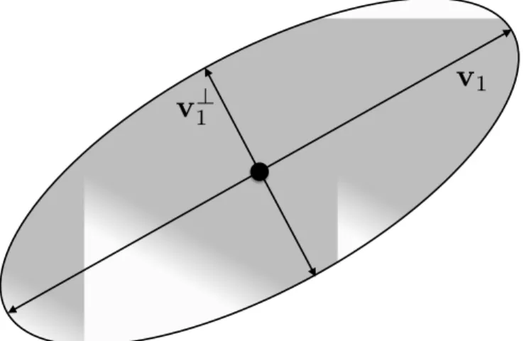
Li-Yezzi minimal path models. . . 27 2.8 Visualization for a typical 2D positive definite symmetric tensor by
an ellipse. . . 29 2.9 Comparative minimal paths extraction results by using the isotropic
and anisotropic RIemannian metrics, respectively. . . 30 2.10 Geodesic distance maps with different values of anisotropy ratio. . . 32 2.11 Stencil examples: 4-connexity and 8-connexity stencils on 2D
carte-sian grid.. . . 37 2.12 Example for fast marching front. . . 40 2.13 Illustration for Bellman’s optimality principle. . . 42 2.14 Demonstrations of the Uint balls for Riemannian Metrics and the
respective stencils which are constructed using the method proposed by Mirebeau (2014a). . . 46 2.15 Demonstrations of the Uint balls for Finsler Metrics and the
respec-tive stencils which are constructed using the method proposed by Mirebeau (2014b). . . 48 2.16 Demonstrations of the Uint balls for Finsler Metrics and the
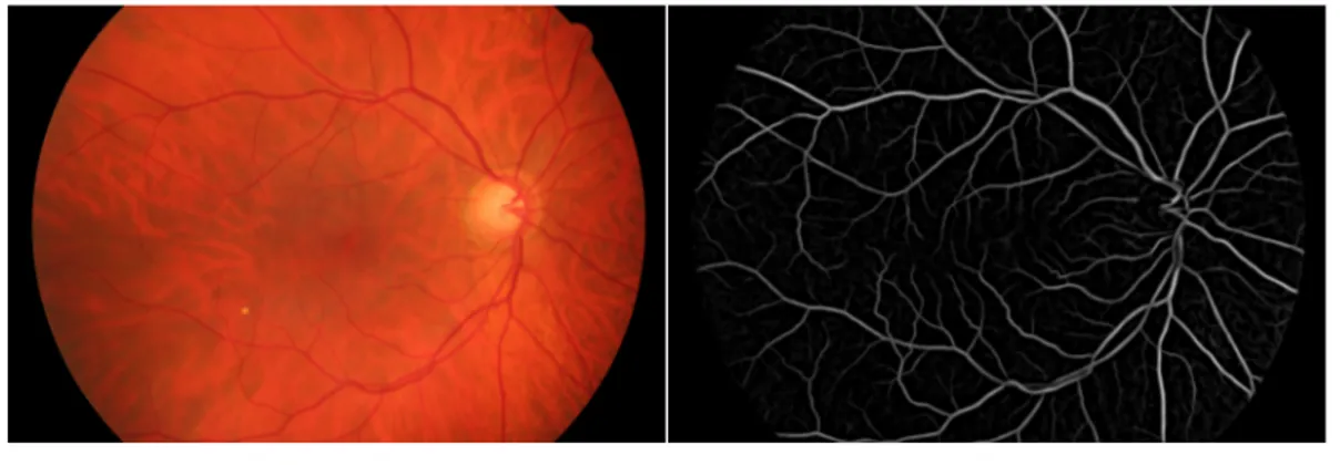
respec-tive stencils which are constructed using the method proposed by Mirebeau (2014b). . . 49 3.1 A Retinal vessel network image (left) and the corresponding vessel
ground truth image (right). . . 53 3.2 An example of retinal vessel image and its vesselness map. . . 54 3.3 Steps of keypoints searching scheme. . . 64 3.4 Keypoints searching result with two path score thresholds. . . 66 3.5 Comparison between our algorithm and the classical KPSM. . . 67
cross and yellow star indicate the initial source points and end points respectively. . . 74 3.10 An example for back-tracked points and the corresponding local
geodesics in a patch of a retinal image. . . 75 3.11 An example for back-tracked points and the corresponding local
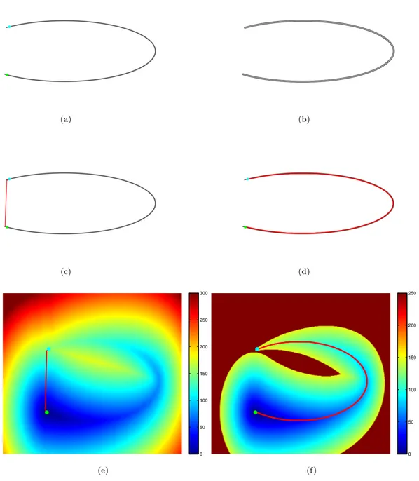
geodesics in a synthetic image. . . 75 3.12 Steps for the proposed Retinal vessel extraction method. . . 80 3.13 Centreline bias correction. . . 80 3.14 Comparative Retinal vessel extraction results by the
Benmansour-Cohen model and the proposed model. . . 81 3.15 Tubular structure preprocessing step. . . 84 3.16 Identifying the segments by removing the branch points and
con-struct the constrained tubular neighbourhood region. . . 85 3.17 Comparative extraction results. . . 86 3.18 Illustration for the proposed algorithm step by step. . . 88 3.19 Segmentation of a retinal image by the proposed method. . . 89 3.20 Details of the segmentation results shown in Fig. 3.19. . . 90 3.21 Improved results by Endpoints Correction. . . 91 4.1 Illustration of the approximation of the flux computation. . . 97 4.2 Illustration for the various regions used in the proposed model in
the course of the fast marching front propagation. . . 101 4.3 Front propagation based on the tensor field Mc in (4.14) for
differ-ent values of anisotropy ratio. . . 103 4.4 The course of the fast marching front propagation using isotropic
fast marching front propagation method . . . 104 4.5 Comparative vessel tree segmentation results from different methods.105 5.1 Minimal path extraction results using different metrics. . . 112 5.2 Visualization for the metrics F1 and Fλ with ↵ = 1 by Tissot’s
indicatrix. . . 114 5.3 Approximating Euler elastica curves by Finsler elastica minimal
paths with uniform speed. . . 120 5.4 Steps for the closed contour detection procedure.. . . 126 5.5 Flexible Finsler minimal paths extraction on ellipse-like curves.. . . 135 5.6 Comparative minimal paths extraction results on Spirals. . . 135 5.7 Finding the nearest lifted candidate to the
orientation-lifted initial source point in terms of geodesic distance associated to data-driven Finsler elastica metric. . . 136
5.8 Finsler elastica minimal paths extraction results.. . . 136 5.9 Comparative closed contour detection results obtained by using
dif-ferent metrics. . . 137 5.10 Closed contour detection results by using only two given physical
positions and the corresponding orientations. . . 138 5.11 Contour detection results with different values of curvature
penal-ization parameter ↵. . . 139 5.12 Perceptual grouping results by the proposed method and Finsler
elastica metric. . . 140 5.13 Perceptual grouping results by the proposed method and Finsler
elastica metric. . . 141 5.14 Perceptual grouping results by the proposed method where three
groups are identified. . . 142 5.15 Comparative blood vessel extraction results on retinal images. . . . 143 5.16 Comparative blood vessel extraction results on fluoroscopy images. . 143 5.17 Comparative arteries vessels extraction results on retinal images. . . 144 5.18 Retinal veins extraction results from different metrics. . . 145 5.19 Comparative blood vessel extraction results on blurred retinal image.145 5.20 Roads extraction results by the proposed Finsler elastica metric in
aerial image blurred by Gaussian noise. . . 146 6.1 Illustration of the Chan-Vese active contours model. . . 150 6.2 Illustration for the U -constrained shape evolution. . . 158 6.3 Tubular neighbourhood regions for ⌧ = 0, where we denote the
neighbourhood regions by red shadow. . . 166 6.4 Shape evolution results of the proposed model with contour
initial-ization and two sampled vertices. . . 169 6.5 Shape evolution results of the proposed model with contour
initial-ization and four sampled vertices. . . 170 6.6 Shape evolution results of the proposed model with three fixed
points initialization.. . . 173 6.7 Comparative segmentation results by the level set based nonlocal
active contours model (Jung et al., 2012) and the proposed model with contour initialization. . . 174 6.8 Comparative segmentation results by the level set based locally
bi-nary fitting model (Li et al., 2008) and the proposed model with fixed points initialization. . . 174
3.1 Comparison of the vessel extraction results for the Benmansour-Cohen model and the proposed minimal path model. . . 82 3.2 Comparison of our segmentation results with the second manual
segmentation on the test set of DRIVE dataset. . . 92 3.3 Comparison of our segmentations Computation time (in Seconds)
with Benmansour and Cohen (2011) model on retinal images from the test set of DRIVE dataset. . . 92 5.1 Computation time (in seconds) and average number of Hopf-Lax
updates required for each grid point by fast marching method with ↵ = 500 and different values of λ on a 3002⇥ 108 grid. . . . 121 6.1 Computation time and evolution steps (ES) required by the
pro-posed method with regional term fCVunder different pairs of (δ, d) in equations (6.54) and (6.56). . . 170
Ω image domain, an open subset of R2, Ω⇢ R2
ˆ
Ω radius-lifted domain ¯
Ω orientation-lifted domain
I a gray level image, an integrable function I : Ω! R I a color image, a vector-valued function I : Ω! R3
x a point in the image domain, x2 Ω y a point in the image domain, y2 Ω Γ a regular curve
γ another regular curve Cx,y a geodesic joining x to y
u vector field, usually defined in the image domain, u : Ω! R2
v vector field, usually defined in the image domain, v : Ω! R2
N unit normal field of a curve M tensor field F geodesic metric r gradient operator r· divergence operator ∆ Laplacian operator ⇤ convolution
Gσ Gaussian function with variance σ
Introduction
Image segmentation plays an essential role in the field of image processing, link-ing low level image processlink-ing procedure like image denoislink-ing, restoration and enhancement to the high level medical imaging applications and computer vision. The basic goal of image segmentation is to partition the image to a collection of components, which generally are disjoint to each other. Image segmentation is still a challenging problem, since different types of images may require different segmentation methods.
There are a large number of segmentation methods have been studied in the past decades. Among these methods, the class of thresholding methods is widely used which are usually taken as the rough segmentation step for the possible refined procedures, thanks to its easy implementation and low complexity. These meth-ods make use of the grey level or color information of each pixel or group of pixels (like image patch) and assign the same label to these pixels with similar properties. However, without the regularization to the connectivity of pixels, these threshold-ing methods often suffer from the problem of sensitivity to noise. Furthermore, thresholding based segmentation methods lack of the ability to incorporate more complicated and useful information, such as texture, shape prior and user interven-tion. More advanced segmentation methods have been devoted to this field,such as the graph based models and the variational deformable models.
Graph-based segmentation methods such as the normalized cut model proposed byShi and Malik (2000), the graph cut-based segmentation method (Boykov and Funka-Lea, 2006) and the random walk segmentation model (Grady, 2006). The formulation of these models assume that the images survive on the discrete domain and regard an image as a graph making up of edges and nodes. The optimalization of the graph-based energies are particularly efficient, for instance, the graph cut minimization methods (Boykov and Kolmogorov, 2004; Kolmogorov and Zabin, 2004). Another advantage of the graph-based segmentation models is the easy
jects with long and thin structures.
Active contours models are designed to minimize curve energy functionals survived on the continuous domain based on the Euler-Lagrange equations and variational principles. The basic idea of the active contours model (Kass et al., 1988) is to deform a curve or a snake to converge to the object boundaries, where the curve is controlled by the internal and external forces. Specifically, the internal force can ensure the active contours to be smooth, while the external force, computed in terms of image data, can attract the active contours toward to the boundaries. Various external forces (Cohen,1991;Cohen and Cohen,1993;Xie and Mirmehdi, 2008; Xu and Prince, 1998) have been proposed to improve the performance of the active contours model. The geometric active contours models (Caselles et al., 1993, 1997) are based on the Euclidean curvature motion flow. In their basic formulation, the active contours are represented by the zero value of a level set function (Osher and Sethian, 1988). These geometric models are able to deal with the topological changes automatically, thanks to the level set-based curve evolution scheme. However, based on the respective Euler-Lagrange equations and gradient descent flows, these active contours models sometimes fall into spurious edges resulted by noise or intensities inhomogeneity. Further, these active contours energies have strong non-convex formulas. Thus it is difficult to find the global minima of the energies.
The minimal path model was proposed by Cohen and Kimmel (1997) to find the global minimum of the geodesic energy by solving a nonlinear partial differential equation (PDE), instead of the linear Euler-Lagrange equation which is used in the classical geodesic active contours model (Caselles et al., 1997). The crucial point in this minimal path model is the design of the geodesic metric F, where the curve energy is obtained by integrating F along a regular curve Γ. Once one gets the metric F, the minimal geodesics between any point in the domain and the initial source point can be determined immediately, following the calculation of the geodesic distance map. The original Cohen-Kimmel minimal path model (Cohen and Kimmel,1997) has raised many interactive image segmentation meth-ods via closed contour detection procedures (Appia and Yezzi, 2011; Appleton and Talbot, 2005; Benmansour and Cohen, 2009; Mille et al., 2014), where the common proposal is that the object boundaries are delineated by a set of minimal paths constrained by the user input seeds. Moreover, minimal paths-based models
are particularly suitable for tubular structure extraction (Benmansour and Cohen, 2011; Li and Yezzi,2007).
Within this thesis, various suitable metrics F are designed for different tasks of tubular structure extraction for retinal blood vessels extraction and active contours for image segmentation. The technical contributions are outlined in Chapters 3 to 6. In chapter 2 we give the introduction to deformable models which form the basis of this thesis. The main structure is outlined as follows:
• Chapter2introduces the scientific background of this thesis: the deformable models including the active contours models and the minimal path models. We start this chapter from the analysis of the curve energy of the original active contours model proposed byKass et al. (1988). Then the classical ac-tive contours models are introduced along the line of how these models are able to solve the problems suffered by the original active contours model. In this chapter, the level set method and the fast marching method, which are the numerical tools for the active contours models and for the minimal path models, are also discussed respectively. Specifically, we make use of the state-of-art anisotropic fast marching methods introduced in (Mirebeau, 2014a,b) as the Eikonal solvers associated to the designed metrics that are used through this thesis. The details of the construction of the adaptive stencils are presented in Section2.4.4.
• Chapter3demonstrates the power of the Eikonal PDE-based minimal paths for the task of tubular structure segmentation, especially for retinal blood vessels extraction. We address the problems of finding both the centrelines and boundaries of the vessels simultaneously that are suffered by the existing state-of-the-art minimal path models.
– Section3.2discusses the optimally oriented flux filter (Law and Chung, 2008) which is taken as the tubular anisotropy descriptor in this thesis for tubular structure extraction. This filter can be used to detect the probability of each pixel belonging to a vessel and the optimal orienta-tion for each vessel point.
– Section 3.3introduces the details of the construction of the anisotropic radius-lifted Riemannian metric proposed by Benmansour and Cohen (2011). In the basic formulation, each point of a 3-D radius-lifted mini-mal path associated to this metric includes three components: the first two coordinates represent the physical position and the last coordinate is the value of the corresponding vessel radius value.
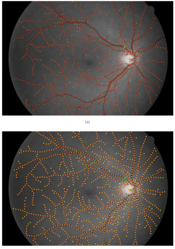
– Section 3.4 introduces a mask-based keypoints detection method for automatic vessel tree extraction and its application for retinal vessel tree extraction. This model only requires one initial source point and
based minimal path model for interactive retinal vessel extraction. This dynamic Riemannian metric is computed by using the local back-tracked geodesic and the consistency of the additional image feature informa-tion. The main goal of this model is to extract a geodesic along which the image feature varies slowly. In this section, we show that this prop-erty is very helpful for interactive retinal blood vessel extraction. We introduce a region-constrained minimal path model to obtain both the centrelines and boundaries of the retinal blood vessel.
– Section3.6presents an automatic method for vessel width measurement based on the region-constrained minimal path model. This method can make use of the binary pre-segmented map to provide a collection of end points and constrained regions to the fast marching method, thus the extracted minimal paths are included inside the constrained region, which can avoid the overlapping extraction problem.
• Chapter4proposes an anisotropic fast marching front propagation method for vessel tree segmentation. The main contribution of this chapter is the construction of dynamic anisotropic Riemannian metric implemented by the anisotropic fast marching method. The dynamic and anisotropic enhance-ment can avoid the leaking problem suffered by the classical isotropic front propagation model, which only relies on the positions.
• Chapter 5 introduces a curvature-penalized minimal path model with an orientation-lifted Finsler elastica metric. This is done by establishing the re-lationship between the Euler elastica bending energy and the geodesic curve energy through a Finsler elastica metric. By solving the Eikonal PDE asso-ciated to the Finsler elastica metric, we can obtain the globally minimizing curvature-penalized minimal geodesics which can be used to approximate the Euler elastica curves.
Based on this Finsler elastica metric, we present the methods for closed con-tour detection, perceptual grouping and tubular structure extraction. The proposed Finsler elastica minimal path model make use of both the informa-tion of the orientainforma-tion and the curvature, thus obtaining better results than the classical minimal path models.
• Chapter 6 introduces a novel non-linear Eikonal-PDE based method for region-based active contours and image segmentation. We transform the
region-based active contours energy to the geodesic curve energy, by a Finsler metric, in terms of the divergence theorem. Therefore, the minimization of the region-based energy is turned to solve the Eikonal PDE associated to the Finsler metrics by the anisotropic fast marching method (Mirebeau,2014b). The minimum of the corresponding Eikonal PDE is very robust and efficient. Traditional region-based active contours energy minimization strategy uses the gradient descent scheme and level set-based curve evolution method, which is sensitive to local minimum and needs a careful treatment to the pa-rameters. In contrast, the proposed method can avoid the problems of sen-sitivity to local minimum and parameters. Moreover, the proposed method is very easy and natural to incorporate the user-provided information. • Chapter 7 summaries the main contributions of this thesis and gives the
Active Contours and Minimal
Paths
Abstract
In their basic formulation, deformable models are designed for the goal of driving a curve, closed or open, to converge to the object boundary according to some variational principles. The class of active contours models is one of the most successful and powerful models in the field of image segmentation. Active contours models have solid mathematical background and well established numerical tools to support various real world applications. Among these active contours models, the Eikonal equation based minimal path model has distinguished advantages, such as global minimum and fast numerical solution, which guarantee the wide use of this model in medical imaging like tubular structure extraction in medical imaging and boundary detection in computer vision.
In this chapter, we briefly discuss the existing well known active contours models, their respective gradient descent flows and the corresponding level set-based curve evolution scheme, and the Eikonal PDE-based minimal path models with differ-ent geodesic metrics as well as the respective numerical fast marching methods associated to these metrics.
work of the active contours/snakes model proposed byKass et al.(1988). The core idea behind this model is to deform a snake to converge at the interesting edges, where a snake is a regular parametrized curve Γ : [0, 1] ! Ω locally minimizing the curve energy:
ESnake(Γ) = Z 1 0 " w1kΓ0(t)k2 + w2kΓ00(t)k2+ P " Γ(t)##dt, (2.1) with appropriate boundary conditions at the endpoints t = 0 and t = 1. Ω is the image domain. Γ0 and Γ00are the first- and second-order derivatives of the curve Γ, respectively. Positive constants w1and w2relate to the elasticity and rigidity of the
curve Γ, hence weight its internal forces. This approach models object boundaries as curves Γ locally minimizing an objective energy functional E that consists of an internal force and an external force. The internal force terms depend on the first-and second-order derivatives of the curves or snakes, first-and respectively account for a prior of small length and of low curvature of the contours. The external force is derived from a potential function P , depending on image features like gradient magnitude, and designed to attracting the active contours or snakes to the image features of interest such as object boundaries. The function P has a small values around the interested image features, where a common P can be computed by
P (x) = g(krI(x)k), 8 x 2 Ω, (2.2) where g is a non-negative decreasing function such as
g(a) = ⌘0+
1 ⌘1+ a
, or g(a) = ⌘0 + exp(−⌘1a), a2 [0, 1), (2.3)
where ⌘0 and ⌘1 are positive constants.
The Euler-Lagrange equation of the energy functional Esnake with respect to the
admissible curve Γ is expressed as
− !1Γ00(t) + !2Γ0000(t) +rP (Γ(t)) = 0, 8 t 2 [0, 1], (2.4)
which means that a curve Γ⇤ locally minimizing the active contours energy E snake
defined by
Γ0000(t) = @
4
@t4Γ(t), 8t 2 [0, 1].
In order to find the locally optimal contour Γ⇤, applied the gradient descent method to iteratively minimize Esnake (2.4), which introduced a family of curve Γ(⌧,·) :
[0,1) ⇥ [0, 1] ! Ω with respect to time ⌧.
The curve evolution formula associate to ⌧ can be expressed as @Γ @⌧ = !1Γ 00 − !2Γ0000 | {z } Regular Term − rP (Γ). | {z }
External Vector Field
(2.5)
One expects the curve Γ to delineate the desired boundaries when ⌧ ! 1. The regular term of (2.5) enforce the curves to be smooth, thus referred to an internal force
Fsmooth:= !1Γ00− !2Γ0000. (2.6)
The termsrP is used to attract the active contours to the boundaries. This forms the external force of the active contours model:
FExt :=−rP. (2.7)
Generally, the external vector field rP , associated to the external force, has a small supported domain which is around the object boundaries which may lead the active contours model to be sensitive to initial curves.
The efforts for the improvements of classical active contours model (Kass et al., 1988) are mainly devoted to three drawbacks: 1) sensitive to initialization, 2) difficult to deal with topological changes of the active contours, and 3) strong non-convex curve functional energy.
• Regarding the initialization of this classical active contours model, it requires an initial guess close to the desired image features, and preferably enclos-ing them because energy minimization tends to shorten the snakes. The introduction of an expanding balloon force allows to be less demanding on the initial curve given inside the objective region (Cohen, 1991). Moreover, extended vector field approaches have been studied in (Cohen and Cohen, 1993; Li and Acton, 2007; Xie and Mirmehdi, 2008; Xu and Prince, 1998) to enlarge the supported domain of the external force FExt, which will be
introduced in next sections.
• The issue of topology changes led, on the other hand, to the development of active contour methods, which represent object boundaries as the zero level set (Osher and Sethian,1988) of the solution to a PDE (Caselles et al.,1993,
Lagrange equation (2.4) meaning that only the local minimum of Esnake can
be obtained. This may result that the minimizing curves Γ⇤ are sensitive
to noise and spurious edges. Cohen and Kimmel (1997) suggested a way to to obtain the global minimum of a variant of the energy functional ESnake
through the solution of the Eikonal PDE. This variant energy is the fa-mous geodesic energy (Caselles et al., 1997) that removes the second-order derivative term Γ00. Moreover, the geodesic energy is independent of the
pa-rameterization of the curve, a problem that is suffered by the classical active contours model (Kass et al., 1988).
2.1.2
Active Contours Model with Ballon Force
Cohen(1991) introduced a additional external force for the active contour models. This external force drives the contour to deform as a balloon in a inflation way. In the basic formulation, the new external ballon force can be expressed as
FBallon := cN , (2.8)
where N denotes the normal vector of the curve Γ.
Note that the balloon force FBallon (2.8) can be obtained by minimizing the
fol-lowing region-based functional
c Z
Ri
dx,
where c is a constant and Ri is the region inside the curve Γ, i.e., Γ = @Ri.
Based on the ballon force FBallon (2.8), Cohen (1991) presented a new external
force
FExt = FBallon− c2 rP
krP k, (2.9)
where c2 is a constant. The parameter c2 should be a little larger than c. Hence
the edge points can stop the evolution of the curve under the control of FExt (2.9).
With the additional ballon force FBallon, spurious edges produced by noise can be
avoided. Moreover, the initial curve can be placed far from the boundaries, thus the ballon force based active contours model is insensitive to the initialization.
2.1.3
Active Contours with Distance Vector Flow
Cohen and Cohen (1993) presented a new external force making use of the pre-detected edge points to reduce the problem of sensitivity to the initializations of the classical active contours model (Kass et al., 1988). This method firstly computes a Euclidean distance map D for each point x2 Ω where D(x) denotes the Euclidean distance value of x to the nearest edge points.
By the use of a decreasing function g (2.3), the external force of the distance vector field can be expressed as
FExt(x) :=−g0
"
D(x)#rD(x), 8 x 2 Ω. (2.10) where rD is the gradient map of D, which points to the edge points. This gradient vector field can be considered as the distance competition such that the curve will be attracted to its nearest edge points. The edge points can be detected by using various edge detectors such as the Canny detector (Canny, 1986) or the higher order steerable edge detector (Freeman and Adelson, 1991; Jacob and Unser, 2004).
2.1.4
Active Contours with Gradient Vector Flow
Xu and Prince (1998) proposed a new external force for active contours evolution scheme based on the diffused gradient vectors of the edge map. The basic idea is to diffuse the image gradient information to the whole image domain Ω, leading to an insensitive initialization for the active contours model.
Let H = (u, v) : Ω! R2 be the expected diffused gradient vector field. H can be
obtained by solving the following minimization problem:
min u,v 8 > > > < > > > : µ Z Ω ⇣ kru(x)k2+krv(x)k2⌘dx | {z } † + Z Ωkrh(x)k 2 kH(x) − rh(x)k2dx | {z } ‡ 9 > > > = > > > ; (2.11)
where h(·) = krI(·)k is the norm of the image gradient rI(·) and µ is a positive constant that is used to balance the importance between terms† and ‡. The term † ensures the smoothness of the vector field H and ‡ is the image data term. At the edge points, minimizing (2.11) implies that H⇡ rh since at these points the value of the normkrhk is very large.
The gradient vector field H satisfies the Euler-Lagrange equation of (2.11). Xu and Prince (1998) suggested to use the following gradient descent equation to
(a) Edge map
(b) Gradient vector field
computed the desired vector field H for any x = (x, y)2 Ω: @u @⌧(x) = µ∆u(x)− (u(x) − hx(x))krh(x)k 2, (2.12) @v @⌧(x) = µ∆v(x)− (v(x) − hy(x))krh(x)k 2, (2.13)
where hx = @h@x and ∆ is the Laplacian operator. If point x is in
homoge-neous region, the norm krh(x)k ⇡ 0 and (u(x) − hx(x))krh(x)k2 or (v(x)−
hy(x))krh(x)k2 will vanish. Thus in such region, the components u and v of
vec-tor field H are computed by the diffusion equation which enforce the smoothness of H. In contrast, if point x is at the vicinity region of the image boundaries, one has
u(x)⇡ hx(x) and v(x)⇡ hy(x).
Then the gradient vector flow force FGVF can be expressed as
FGVF := H, (2.14)
or more generally, the gradient vector flow can be computed by the normalized gradient vector field of H
FGVF(x) :=
H(x)
kH(x)k, 8x 2 Ω. (2.15) The gradient vector field H extends the narrow band supported domain of the original image gradient vector field rh to the whole domain Ω, thus the active contours model controlled by the gradient vector field H is insensitive to initializa-tions. In other words, one can place the initial curve far from the object boundaries (Xu and Prince,1998).
2.2.1
Level Set Method
In its basic formulation, a level set function is a scalar embedding function, the values of which have opposite signs inside and outside the closed curves. A family of time dependent curves Γ : [0,1)⇥[0, 1] ! Ω is represented by the corresponding zero-level set of φ : [0,1) ⇥ Ω ! R:
Γ ={x; x 2 Ω, φ(⌧, x) = 0}. (2.16) In Fig.2.2, we show an example for a level set function. Fig.2.2a shows a contour indicated by black curve. Fig.2.2b shows the implicit representation of the curve in Fig.2.2a by zero value of the level set function and Fig.2.2c is the 3D visualization of the level set function.
Let us consider the basic curve evolution equation(Caselles et al.,1997;Osher and Sethian,1988) in terms of
@Γ
@⌧ = fN , (2.17)
where ⌧ denotes the time, f is a given scalar function, andN is the normal vector of the curve Γ. According to (2.16), one has
φ(⌧, Γ) = 0, (2.18) which yields ⌧ rφ,@Γ @⌧ 2 +@φ @⌧ = 0 (2.19)
Recalling that the curve Γ is defined as the zero-level set of the scalar function φ, the normal vectorN of Γ can be interpreted by
N = rφ
krφk. (2.20)
Thus one obtains
@φ @⌧ =− ⌧ rφ, f rφ krφk 2 =−f krφk, (2.21)
The level set function φ should be reinitialized as a signed distance map in the course of the level set evolution (Osher and Sethian, 1988; Sussman et al., 1994). As discussed in (Sussman et al.,1994), at the time ⌧0, the level set reinitialization
can be done by solving the following time-dependent PDE ( @ @⌧ = sign(φ ⌧0)(1− kr k), (0,·) = φ(⌧0,·), (2.22) where φ⌧0(·) = φ(⌧
0,·) and the new level set function ˜φ is equal to the solution
at the steady state of (2.22).
Note that the level set function can also be reinitialized by using the solution ' of the Eikonal PDE: (
kr'(x)k = 1, 8x 2 Ω\Ψ0,
'(x) = 0, 8x 2 Ψ0,
(2.23) where Ψ0 is defined as a collection
Ψ0 :={x 2 Ω; (⌧0, x) = 0}.
The desired reinitialized level set function ˜φ can be computed by ˜
φ = sign(φ⌧0) ' .
The Eikonal PDE (2.23) can be solved the isotropic fast marching method (Sethian, 1996,1999) or by the GPU-accelerated fast sweeping method proposed by (Weber et al., 2008).
Li et al. (2010) proposed a new method to avoid the level set reinitialization operation. This is done by minimizing the following term
Z
Ω
PRegu(krφ(x)k)dx, (2.24)
wherePRegu is a potential function. One possible choice for this potential function,
as suggested In (Li et al., 2010), can be formulated as PRegu(x) =
1
2(x− 1)
2. (2.25)
Minimizing (2.24) with respect to the potential function formulated in (2.25) is used to enforce krφk ⌘ 1, which implies that φ is a distance function. However, the potential function PRegu (2.25) may suffer from the side effect problem (Li et al.,2010). To solve this problem,Li et al.(2010) designed a double-well potential
2.2.2
Geometric Active Contours
The geometric active contours model was proposed by Caselles et al. (1993) and Malladi et al. (1994) for object boundary detection, by driving the contours ac-cording to the following flow:
@Γ
@⌧ = g ( + c)N , (2.26)
where g is the image data function defined in (2.3), c is a positive constant and is the curvature of curve Γ. Actually, g plays the role of stopping function which can stop the evolution of Γ when it arrives at the real object boundaries, since at these boundaries one has g ⇡ 0.
The curve evolution flow (2.26) is actually based on the Euclidean curvature flow or Euclidean heat flow
@Γ
@⌧ = N , (2.27)
which can shorten and smooth the curve Γ. This flow can drive the curve Γ to minimize its curve length functional
Z 1 0 kΓ
0(t)
kdt
in the gradient direction (Caselles et al.,1993). By incorporating the curve Γ into the level set function φ, we can obtain the level set evolution equation according to (2.26) as follows: @φ @⌧ = ✓ r ·✓ rφ krφk ◆ + c ◆ gkrφk, (2.28)
where r · u denotes the divergence value of vector u. This level set evolution equation is based on the fact that
=r ·✓ rφ krφk
◆ .
Corresponding to the general level set-based curve evolution flow (2.21), we have that the speed function f = g(c + ). When the curve Γ is far from the boundary, the stopping function g can be considered as a positive constant such that the
(a) A contour −40 −20 0 20 40 60 80
(b) Level set function
(c) 3D visualization of the level set function
Figure 2.2: An example for level set function. (a) A contour indicated by a black closed curve. (b) Implicit representation for the curve demonstrated in (a) by the zero value of the level set function. (c) 3D visualization for the level set function shown in
(b).
(a) Initial contour
(b) Intermediate result (c) Final result
Figure 2.3: Image Segmentation by using geodesic active contours. (a) Original image and initial contour. (b) Intermediate segmentation result. (c) Final segmentation
result.
the ballon force cN . When Γ is close to the boundaries, one has g ⇡ 0 such at the evolution of the contour will be terminated.
This level set based geometric active contours model can deal with curve topology changes automatically. The initial curve can be placed outside the object and far from its boundaries. Moreover, starting from a convex curves, one can obtain a non-convex final contours represented by the zero value of level set function φ.
2.2.3
Geodesic Active Contours
The famous geodesic active contours model proposed byCaselles et al.(1997) aims at finding a locally optimal curve Γ⇤ to (locally) minimize the geodesic energy in a Riemannian space with a isotropic Riemannian metric
EGAC(Γ) =
Z 1 0
P (Γ(t))kΓ0(t)kdt, (2.29)
with potential function P . This energy removed the second-order derivative term of the curve Γ from the classical snakes energy ESnake in (2.1). The gradient flow of
the geodesic energy EGAC can be expressed as (Caselles et al.,1997;Kichenassamy et al., 1995)
@Γ
@⌧ = (g +hrg, N i) N . (2.30) The term ofhrg, N i can push the curve toward the valley of the stopping function g (Caselles et al., 1997). This property is very useful for purpose of detecting a boundary that passes through the regions with inhomogeneous intensities and high noise.
In order to improve the performance of the geodesic gradient flow (2.30) to deal with the detection of boundaries with high curvature, Caselles et al. (1997) give the gradient flow by adding a constant c as
@Γ @⌧ =
⇣
(g + c) +hrg, N i⌘N . (2.31) The behaviour of this geodesic gradient flow can be divided to two cases:
• When the curve is close to the boundary, the stopping function g is degener-ated to a constant and rg = 0. The gradient flow (2.31) is identical to the Euclidean heat flow: the curve tends to shrink to a point.
• When the curve is close to the boundary, the stopping function g have small values and the force hrg, N i will push or pull the curve to the explicit boundary where each point xb at the boundary obeying that rg(xb) = 0.
By combining with the level set function φ, we can obtain the level set evolution equation: @φ @⌧ = (g + c)div ✓ rφ krφk ◆ krφk + hrg, rφi, (2.32) which is a geometric front propagation approach. In Fig.2.3 we show the segmen-tation result using the geodesic active contours model. Fig. 2.3a is the original image with initial contour indicated by red curve, Fig. 2.3b is the intermediate result and Fig. 2.3c is the final segmentation contour.
Figure 2.4: Geodesic active contours for object segmentation with concave region using a small value of the constant c.
Note that the constant c in the flows (2.26) and (2.30) should be treated carefully. This parameter is used to address the possible shortcuts problem when dealing with the segmentation task for the object with concave region. In this case, when the value of the constant c is very small, the curve evolution might be stopped before it follows the expected boundary. We illustrate this shortcuts problem in Fig. 2.4. However, if the value of c is too large, some parts of the active contours may stop inside the object.
2.2.4
Alignment Active Contours
Kimmel and Bruckstein (2003) and Kimmel (2003) presented a novel active con-tours model with the energy function consisting of a alignment term:
EAlign(Γ) =
Z 1
0 hrI(Γ(t)), N ikΓ 0(t)
kdt, (2.33)
where rI is the gradient vector field of the given image I. This model adds the anisotropy of the path to the energy such that tangents of the obtained optimal curve should be consistent to the image gradient vector field rI. The gradient flow of EAlign can be expressed as
@Γ
where ∆I is defined for each x = (x, y)2 Ω as ∆I(x) = @ 2I @x2(x) + @2I @y2(x).
A robust version of the energy EAlign is proposed byKimmel (2003);Kimmel and Bruckstein (2003): ERalign(Γ) = Z 1 0 6 6 6hrI (Γ(t)), N i 6 6 6 kΓ0(t)kdt (2.35) with the gradient flow of
@Γ @⌧ =
hrI, N i
khr, N ik∆IN . (2.36)
The values of the term khrI,N ikhrI,N i denote actually the sign map of the align term hrI, N i.
where S1 = [0, ⇡) or [0, 2⇡).
2.3.1
From Active Contours to Eikonal PDE-based
Mini-mal Paths
The difficulty of minimizing the non-convex snakes energy (Kass et al., 1988) ESnake(Γ) = Z 1 0 " w1kΓ0(t)k2 + w2kΓ00(t)k2+ P " Γ(t)##dt, (2.37) leads to important practical problems, since the curve optimization procedure is often stuck at unexpected local minima of the energy functional ESnake (2.37),
making the results heavily rely on curve initialization and sensitive to image noise. This is still the case for the level set approach on geometric or geodesic active contours (Caselles et al.,1993,1997;Malladi et al.,1995). In order to address this local minimum sensitivity issue, Cohen and Kimmel (1997) proposed an Eikonal PDE-based minimal path model, with goal of finding the global minimum of the geodesic energy which is similar to that used in (Caselles et al., 1997), in which the penalty associated to the second-order derivative of the curve was removed from the snakes energy. Thus the reduced energy functional is
Z 1 0
⇣
w + P"Γ(t)#⌘kΓ0(t)k dt,
the local minimizer of which was proved to be a geodesic in (Caselles et al.,1997). Alternately,Cohen and Kimmel(1997) proposed a non-linear PDE based approach to find the global minimizer of this geodesic energy. Thanks to this approach, a fast, reliable and globally optimal numerical method allows to find the energy minimizing curve with prescribed endpoints; namely the fast marching method (Sethian, 1999), based on the formalism of viscosity solutions to Eikonal PDE. These mathematical and algorithmic guarantees of Cohen and Kimmel’s minimal path model have important practical consequences, leading to various approaches for image analysis and medical imaging (Benmansour and Cohen, 2011; Cohen, 2001; Deschamps and Cohen, 2001; Li and Yezzi, 2007; Mille et al., 2014; Peyr´e et al., 2010).