Topics in mathematical morphology for multivariate images

HAL Id: pastel-00820581

https://pastel.archives-ouvertes.fr/pastel-00820581

Submitted on 6 May 2013

HAL is a multi-disciplinary open access

archive for the deposit and dissemination of

sci-entific research documents, whether they are

pub-lished or not. The documents may come from

teaching and research institutions in France or

abroad, or from public or private research centers.

L’archive ouverte pluridisciplinaire HAL, est

destinée au dépôt et à la diffusion de documents

scientifiques de niveau recherche, publiés ou non,

émanant des établissements d’enseignement et de

recherche français ou étrangers, des laboratoires

publics ou privés.

Topics in mathematical morphology for multivariate

images

Santiago Velasco-Forero

To cite this version:

Santiago Velasco-Forero.

Topics in mathematical morphology for multivariate images.

General

Mathematics [math.GM]. Ecole Nationale Supérieure des Mines de Paris, 2012. English. �NNT :

2012ENMP0086�. �pastel-00820581�

!

"

#

$

!

École doctorale n

432 : Sciences des Métiers de l’Ingénieur

Doctorat ParisTech

T H È S E

pour obtenir le grade de docteur délivré par

l’École nationale supérieure des mines de Paris

Spécialité « Morphologie Mathématique »

présentée et soutenue publiquement par

Santiago Velasco-Forero

le 14 juin 2012

Contributions en morphologie mathématique pour l’analyse

d’images multivariées

Directeur de thèse : Jesús ANGULO

Jury

M. Dominique JEULIN,Professeur, CMM-MS, Mines ParisTech Président

M. Jos B.T.M. ROERDINK,Professeur, University of Groningen Rapporteur

M. Pierre SOILLE,Directeur de recherche, Joint Research Centre of the European Commission Rapporteur

M. Jón Atli BENEDIKTSSON,Professeur, University of Iceland Examinateur

M. Fernand MEYER,Directeur de recherche, CMM, Mines ParisTech Examinateur

M. Jean SERRA,Professeur émérite, ESIEE, Université Paris-Est Examinateur

M. Jesús ANGULO,Chargé de recherche, CMM, Mines ParisTech Examinateur

MINES ParisTech

Centre de Morphologie Mathématique, Mathématiques et Systèmes 35, rue Saint-Honoré, 77305 Fontainebleau, France

Acknowledgements

I would like to express my deepest gratitude to my advisor, Dr. Jesús Angulo, for his guidance, motivation and the research freedom he gave me during my Ph.D. studies. It was indeed a huge privilege to be his student.

I am grateful to Dr. Fernand Meyer, director of the Centre for Mathematical Morphology (CMM) at the Ecole des Mines de Paris, for his continuous support. My research activities were also partially supported by the IHMO Project (ANR-TecSan’07), funded by the French National Research Agency. I would also like to thank my thesis reporters (Dr. Jos Roerdink and Dr. Pierre Soille) for their valuable suggestions and contributions that helped me to improve the quality of this document with their objective and pertinent comments. I am highly grateful to Dr. Jón Benediktsson, Dr. Dom-inque Jeulin, Dr. Fernand Meyer and Dr. Jean Serra, who have served in my committee and have contributed many useful comments before and during my dissertation.

Much of the inspiration for this work came during a three months visit to the Joint Research Center of the European Commission. I am very grateful to the members of the Institute to the Protection and Security of the Citizen (IPSC), particularly to Dr. Pierre Soille for our several enlightening conversations.

At Fontainebleau, I could not have asked for a more fun and interesting group of people to work with: Andres, Bea, Bruno, Catherine, Charles, Christoph, Dominique, El Hadji, Estelle, Etienne, Fernand, François, Guillaume, Hellen, Joana, Jorge, Jean, John, Julie, Louise, Luc, Matthieu, Michel, Petr, Serge, Torben, Vincent, Xiwei, and many others. Thank you all for making CMM a place where I truly enjoyed coming to work. Also, I would like to thank Julie who has been a great source of “bio-energy". She has supported me in hundreds of ways throughout the development and writing of this dissertation.

I also take this opportunity to mention my “boricuas" friends: Angel, Ana, Andrea, Catalina, Diana, Karen, Leidy, Marggie, Maider, Oscar, Pedro Alejo, Victor and Yolanda, for encourage me to cross the Atlantic few years ago.

At last, but not least, I would like to dedicate this thesis to my family: Esta tesis es para ust-edes.... familia! Carlitos, Foreman, Lola, Papi, Mami, Carloncho, Bubita, Violeta, Paula Victoria y Carolina. Gracias por el constante apoyo, eterno amor y el ejemplo de superación que me han dado, día tras día.

Résumé

Cette thèse contribue au domaine de la morphologie mathématique et illustre comment les statis-tiques multivariées et les techniques d’apprentissage numérique peuvent être exploitées pour con-cevoir un ordre dans l’espace des vecteurs et pour inclure les résultats d’opérateurs morphologiques au processus d’analyse d’images multivariées. En particulier, nous utilisons l’apprentissage super-visé, les projections aléatoires, les représentations tensorielles et les transformations conditionnelles pour concevoir de nouveaux types d’ordres multivariés et de nouveaux filtres morphologiques pour les images multi/hyperspectrales. Nos contributions clés incluent les points suivants :

• Exploration et analyse d’ordres supervisés, basés sur les méthodes à noyaux.

• Proposition d’un ordre non supervisé, basé sur la fonction de profondeur statistique calculée par projections aléatoires. Nous commençons par explorer les propriétés nécessaires à une image pour assurer que l’ordre ainsi que les opérateurs morphologiques associés, puissent être interprétés de manière similaire au cas d’images en niveaux de gris. Cela nous amènera à la notion de décomposition en arrière plan / premier plan. De plus, les propriétés d’invariance sont analysées et la convergence théorique est démontrée.

• Analyse de l’ordre supervisé dans les problèmes d’appariement par forme de référence, qui correspond à l’extension de l’opérateur tout-ou-rien aux images multivariées grâce à l’utilisation de l’ordre supervisé.

• Discussion sur différentes stratégies pour la décomposition morphologique d’images. Notam-ment, la décomposition morphologique additive est introduite comme alternative pour l’analyse d’images de télédétection, en particulier pour les tâches de réduction de dimension et de clas-sification supervisée d’images hyperspectrales.

• Proposition d’un cadre unifié basé sur des opérateurs morphologiques, pour l’amélioration de contraste et pour le filtrage du bruit poivre-et-sel.

• Introduction d’un nouveau cadre de modèles Booléens multivariés par l’utilisation d’une for-mulation en treillis complets. Cette contribution théorique est utile pour la caractérisation et la simulation de textures multivariées.

Abstract

This thesis contributes to the field of mathematical morphology and illustrates how multivariate statistics and machine learning techniques can be exploited to design vector ordering and to include results of morphological operators in the pipeline of multivariate image analysis. In particular, we make use of supervised learning, random projections, tensor representations and conditional transformations to design new kinds of multivariate ordering, and morphological filters for color and multi/hyperspectral images. Our key contributions include the following points:

• Exploration and analysis of supervised ordering based on kernel methods.

• Proposition of an unsupervised ordering based on statistical depth function computed by ran-dom projections. We begin by exploring the properties that an image requires to ensure that the ordering and the associated morphological operators can be interpreted in a similar way than in the case of grey scale images. This will lead us to the notion of background/foreground decomposition. Additionally, invariance properties are analyzed and theoretical convergence is showed.

• Analysis of supervised ordering in morphological template matching problems, which corre-sponds to the extension of hit-or-miss operator to multivariate image by using supervised ordering.

• Discussion of various strategies for morphological image decomposition, specifically, the ad-ditive morphological decomposition is introduced as an alternative for the analysis of remote sensing multivariate images, in particular for the task of dimensionality reduction and super-vised classification of hyperspectral remote sensing images.

• Proposition of an unified framework based on morphological operators for contrast enhance-ment and salt-and-pepper denoising.

• Introduces a new framework of multivariate Boolean models using a complete lattice formula-tion. This theoretical contribution is useful for characterizing and simulation of multivariate textures.

Contents

Contents 9

List of Figures 13

1 Introduction 17

1.1 Motivation . . . 17

1.2 Order and Mathematical morphology . . . 20

1.3 Why do we need order? . . . 22

1.4 Multivariate Ordering . . . 23

1.5 Thesis overview and main contributions . . . 25

I

Learning Ordering for Multivariate Mathematical Morphology

29

2.2 Scalar images . . . 31

2.3 Morphological transformations . . . 32

2.3.1 Dilation and erosion . . . 32

2.3.2 Opening and closing . . . 33

2.3.3 Contrast mappings . . . 36

2.3.4 Morphological center . . . 36

2.3.5 Geodesic reconstruction, derived operators, leveling. . . 36

2.3.6 Residue-based operators . . . 39

2.4 Morphological Segmentation . . . 43

3 Preliminary Notions 47 3.1 Introduction. . . 47

3.2 Notation and representation . . . 48

3.2.1 Notation. . . 48

3.2.2 Spectral representations . . . 48

3.3 Mathematical morphology in multivariate images . . . 50

3.4 Ordering in vector spaces . . . 50

3.4.1 Complete lattices and mathematical morphology . . . 51

3.4.2 Preorder by h-function. . . 53 4 Supervised Ordering 55 4.1 Introduction. . . 55 4.2 Complete lattices in Rd _{. . . . 56} 4.2.1 Basic Definitions . . . 56 4.2.2 Reduced Ordering . . . 56 4.2.3 h-supervised ordering . . . 57

4.3 Learning the h-supervised ordering . . . 58

4.3.1 Kriging . . . 58

4.3.2 Support Vector Machines . . . 60

10 CONTENTS

4.3.3 Kriging vs. SVM . . . 62

4.4 Morphological operators and h-supervised ordering . . . 63

4.5 Applications to hyperspectral image processing . . . 64

4.5.1 Influence of training set in h-ordering . . . 64

4.5.2 Extracting spatial/spectral structures . . . 65

4.5.3 Duality between background and foreground . . . 65

4.5.4 Multi-target morphological-driven classification . . . 66

4.6 Conclusions on supervised ordering . . . 67

5 Hit-or-miss transform in multivariate images 81 5.1 Introduction. . . 81

5.2 Hit-or-Miss Transform in Multivariate Images . . . 82

5.2.1 Hit-or-Miss Transform in Binary Images . . . 82

5.2.2 Hit-or-miss Transform in supervised h-orderings . . . 83

5.3 Applications to Multivariate Images . . . 84

5.3.1 Geometric Pattern Problem . . . 84

5.3.2 Ship Detection in high-resolution RGB images. . . 86

5.4 Conclusions on supervised multivariate hit-or-miss . . . 86

6 Unsupervised morphology 89 6.1 Introduction. . . 89

6.2 Statistical depth functions . . . 90

6.2.1 Definition . . . 90

6.2.2 Projection depth function . . . 91

6.2.3 Equivalence in Elliptically Symmetric Distribution . . . 92

6.3 MM using projection depth functions. . . 94

6.3.1 Morphological operators and depth h-mapping . . . 98

6.3.2 Properties . . . 99

6.4 Applications to multivariate image processing . . . 101

6.4.1 Image enhancement . . . 102

6.4.2 Image Simplification . . . 103

6.4.3 Image segmentation . . . 103

6.5 Conclusions . . . 104

II

Contributions to morphological modeling

107

7.1.1 Main contributions and chapter organisation . . . 111

7.2 Additive Morphological Decomposition . . . 112

7.2.1 Notation. . . 112

7.2.2 Basic Morphological Transformation . . . 112

7.2.3 Morphological Reconstruction. . . 114

7.2.4 Additive Morphological Decomposition. . . 115

7.3 Tensor Modeling . . . 117

7.3.1 Introduction . . . 117

7.3.2 Tensor Decomposition . . . 117

7.3.3 Tensor Principal Component Analysis (TPCA) . . . 118

7.3.4 Equivalence with PCA . . . 119

7.3.5 Modeling additive morphological decomposition with TPCA. . . 119

7.4 Experiments. . . 121

7.4.1 Data Description and Experimental Setup . . . 121

CONTENTS ₁₁

7.4.3 Results and discussion . . . 128

7.5 Conclusions of the chapter . . . 130

8 Conditional Mathematical Morphology 131 8.1 Introduction. . . 131

8.2 Brief review . . . 133

8.3 Conditional toggle mapping . . . 136

8.4 Experiments. . . 143

8.4.1 Salt & pepper noise reduction. . . 143

8.4.2 Comparison with the state of the art . . . 145

8.4.3 Image enhancement . . . 145

8.5 Conclusions and Perspectives of this chapter. . . 152

9 Multivariate Chain-Boolean models 155 9.1 Introduction. . . 155

9.2 Chain compact capacity . . . 156

9.3 From Boolean Random Model to Chain Boolean Random Models . . . 158

9.3.1 Notation. . . 158

9.3.2 Binary Boolean Random Model . . . 158

9.3.3 Chain Boolean Random Model . . . 159

9.3.4 Properties . . . 160

9.3.5 h-ordering and h-adjunctions . . . 160

9.4 Experiments. . . 161

9.5 Conclusions of this chapter . . . 162

10 Conclusion and Perspectives 165 10.1 Conclusion . . . 165

10.2 Suggestions for Future Works . . . 166

List of Symbols 170

List of Figures

1.1 Scheme hyperspectral image acquisition. Each pixel of the image contains spectral

information in d-bands. It is denoted as a pixel x 2 Rd_{. . . . . 18}

1.2 Comparison of different spatial resolutions. The spatial resolution indicates the small-est distance between two objects that can be distinguished by the sensor. Note that when the size of the objects is close to the spatial resolution, the object is represented in the image as a single pixel. . . 19

1.3 Increasing in the spatial resolution for different satellites through time. . . 19

1.4 Traditional work-flow for supervised classification or segmentation of hyperspectral images. . . 20

1.5 Pixelwise and spatial-spectral classification. The aim of spatial-spectral approaches is integrating contextual spatial information with spectral information to produces more “real" results in the classification stage. . . 21

1.6 Notation for a binary image, I : E ! {0, 1} . . . 22

1.7 Structuring element SE ⇢ E. Blue and red pixels correspond to {x|SE(x) = 1} illus-trating the spatial neighbourhood induced by the structuring element SE centred at x (red pixel). . . 23

1.8 From binary erosion/dilation to multivariate counterparts . . . 24

1.9 Notation for a d-variate image, I : E ! F. Note that the image I maps each spatial point x to a vector x in Rd _{(represented as a curve). . . . . 25}

1.10 Different ordering strategies which are discussed in the Part I of this thesis: (c) Refer-enced Ordering (d) Supervised Ordering (e) Supervised Ordering and (f) Unsupervised ordering.. . . 26

1.11 Representation of colour values of natural images as vector points in R3 _{. . . . 26}

1.12 Example of proposed unsupervised ordering . . . 27

2.1 Basic morphological transformations: dilation (b) and erosion (c). The structuring element SE is a disk of diameter three pixels. . . 34

2.2 Opening (a) and closing (b) transformations. The structuring element SE is a disk of diameter 3 pixels.. . . 35

2.3 Results of toggle mapping and morphological center. . . 37

2.4 Opening and closing by reconstructions . . . 38

2.5 Leveling transformation. . . 40

2.6 Leveling transformation (b) with a marker given by a Gaussian Filter (a). . . 41

2.7 Morphological gradients . . . 42

2.8 Watershed transform for a given image I with markers point M. . . 44

2.9 Contrast-driven watershed transforms. . . 46

3.1 Scheme of different representation for the spectral information of a multivariate image 49 3.2 Spectral information is associated with vector spaces.. . . 50

3.3 Some vector ordering strategies proposed in the literature. The associated ordering is also illustrated.. . . 52

3.4 The h-ordering (preorder) produces a complete lattice for a given set. . . 54

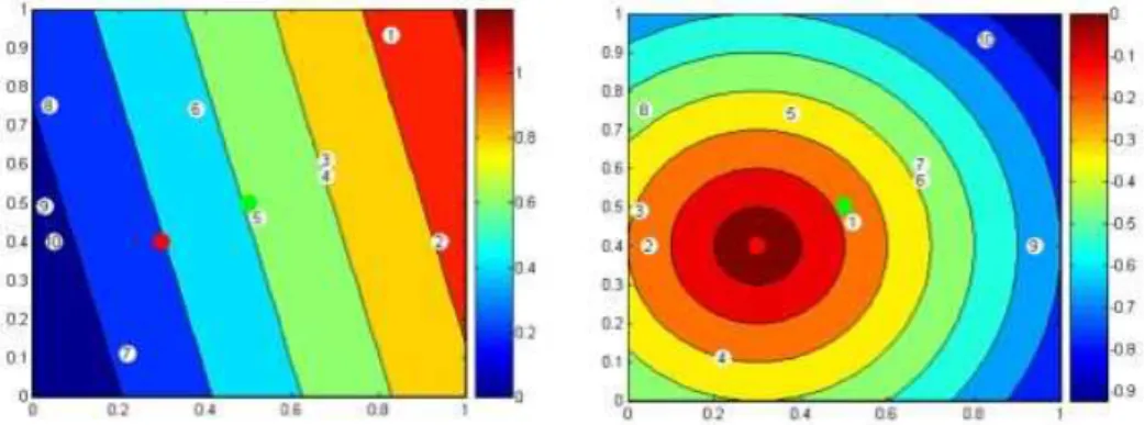
4.1 Scheme of h-supervised function producing a partial ordering on a given original set. 58 4.2 Comparison of h-mappings and their corresponding h-ordering h in R2. . . 59

14 LIST OF FIGURES

4.3 Unitary background and foreground sets: F = f and B = b . . . 60

4.4 Training spectral for Pavia University HSI. . . 62

4.5 Some morphological transformation for Pavia University . . . 68

4.6 Training spectral for Yellowstone Scene. . . 69

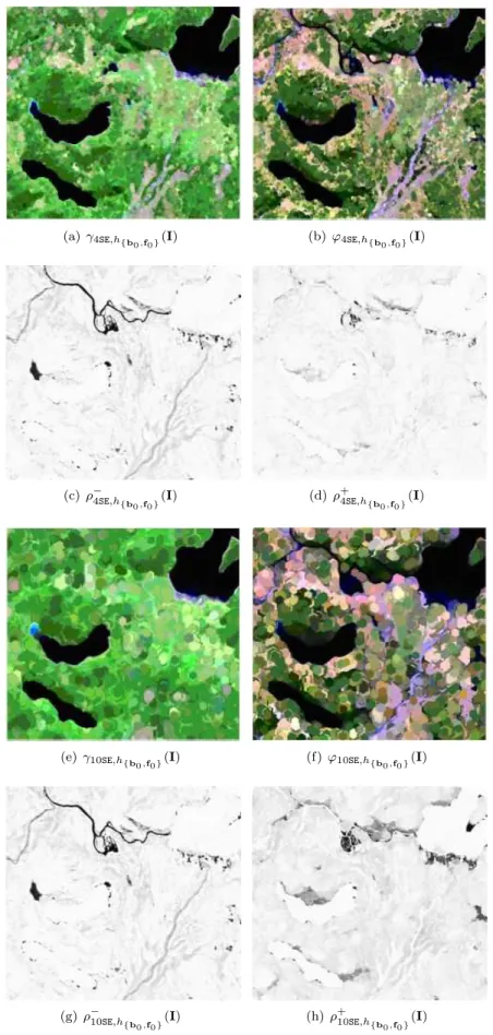
4.7 Morphological transformations for Yellowstone scene.. . . 70

4.8 Toy example in supervised ordering. . . 71

4.9 Training size effect in the supervised ordering for the toy example. . . 71

4.10 Supervised dilation, erosion and gradient for two sets of background/foreground pixels. 72 4.11 Supervised transformation for Yellowstone for the first group of training sets. . . 73

4.12 Supervised transformation for Yellowstone for the second set of training sets. . . 74

4.13 Extraction of specific objects can be performed by using geodesic reconstruction in the supervised ordering. . . 75

4.14 Supervised Leveling for sets of background/foreground pixels. . . 76

4.15 HSI Moffett Field sub-scene using bands {115,70,30}. Reference pixels (background band foreground f) used in the experiments. Curves are plots of the spectral values in the different frequency bands for the reference pixels. . . 77

4.16 Comparison of different supervised morphological operators . . . 78

4.17 Comparison of supervised top-hats. . . 79

4.18 Illustrative example of multiclass supervised ordering. . . 79

4.19 A false colour of the original image is shown using bands number [80,70,30]. Morpho-logical driven-classification using leveling operator with unitary structuring element hexagonal SE. h{T−i,Ti} is obtained using SVM, with polynomial kernel of degree two. 80 5.1 Illustrative example of Hit-or-Miss transform for the set I: HMT (I; SE1, SE2) . . . . 82

5.2 From the binary HMT to the extension for multiband images in the supervised ordering 83 5.3 Example of colour template matching using the proposed multivariate hit-or-miss transform. . . 85

5.4 ROC-curves in the geometric pattern recognition problem . . . 86

5.5 SEs considered in the Bahrain Image. In both scenarios, the sets of pixels background (B1)and foreground (B2)are the same. . . 87

5.6 Ship detection in High-Resolution Samaheej Image using HMT✏ . . . 87

6.1 Intrinsic ordering based on dichotomy background and foreground. . . 90

6.2 Toy example of the computation of (6.1). Projection depth function for a vector x given X is basically the maxima normalised eccentricity for all the possible projection uT_{Xgiven a couple of centrality and variability univariate measures (µ, σ). . . . . . 92}

6.3 “White bird" colour image example. . . 95

6.4 “Canoe" colour image example. . . 96

6.5 “Cuenca map" colour image example.. . . 97

6.6 Example of openings and associated top-hat transformation in the ordering induced by the projection depth function. . . 100

6.7 Projection depth function is invariant to affine transformation in Rd_{. . . . 101}

6.8 Edge enhancement of I using toggle mapping ⌧h(I) in the proposed ordering. Source: http://www.cellimagelibrary.org/ . . . 102

6.9 Original (I), marker (M) and simplification by h-depth vector leveling ΛhI(I, M). The marker M is the product of a h-depth closing followed by an h-depth opening with the SE is a disk of radius 10. . . 103

6.10 h-depth gradient and segmentation by using watershed transformation (in red), where markers are calculated by selecting the minima of strong dynamics in h-depth gradi-ent, with t = .5.. . . 105

6.11 Original multispectral images is the size 200 by 500 pixels in 31 channels. Segmenta-tion for watershed transformaSegmenta-tion with different parameters of dynamics minima of h-depth gradient. . . 105

LIST OF FIGURES ₁₅

6.12 Original hyperspectral image is 610 by 340 pixels on 103-bands. Segmentation by h-depth watershed transformation with different parameters of dynamics minima of

h-depth gradient. . . 106

7.1 Mathematical notation for a 2D multivariate image, I : E ! F . . . 110

7.2 Structuring element SE ⇢ E at x = (i, j) 2 E. MM operators are non-linear neighbourhood-image transforms associated with the structuring element SE. . . 112

7.3 Morphological transformations of a scalar (grey level) image. Original image (a) is a 342 ⇥ 342 pixels in 70-cm-resolution satellite image from the panchromatic band of Quickbird. . . 113

7.4 Example of AMD and ADL for the remote sensing example. . . 116

7.5 Experiment shows clearly that TPCA is equivalent to PCA. . . 120

7.6 Illustration of dimensional reduction stage using additive morphological decomposition.120 7.7 False colour composition of the HSI considered in the experiments. . . 121

7.8 Analysis of AMD in ROSIS Pavia University . . . 122

7.9 First scenario of classification using Indian Pines. Only five pixels per class are selected for the training set. The results show the average and standard deviation in 25 repetitions. . . 124

7.10 Classification maps for the Indian Pines HSI using different approaches. Only five training pixels in nine classes are considered. The classification map is the best result in 25 random repetitions. . . 125

7.11 Behaviour of the overall accuracy in the Pavia University dataset for different mor-phological decompositions and dimensional reduction approach. . . 125

7.12 Classification maps obtained by the different tested methods for Pavia University data set (Overall accuracies are reported in parentheses) . . . 129

8.1 Illustration of gradients and local extrema detectors. . . 134

8.2 Bi-dimensional representation of the evolution in the classical shock filter (8.4) for the Cameraman grey-scale image in (d). . . 135

8.3 Iteration number versus residual between two consecutive iterations of classical and conditional toggle mapping. . . 136

8.4 Conditional vs Classical Dilation. . . 137

8.5 Example showing that the pair conditional operators are not an adjunction in alge-braic sense. . . 138

8.6 The proposed conditional toggle contrast sharpens the signal as well as classical en-hancement method.. . . 141

8.7 The proposed conditional toggle contrast does not produce halos as classical filters in ramp signals. . . 143

8.8 Comparison in free-noisy scenario. . . 144

8.9 Experimental results in PSNR for grey and colour images. . . 146

8.10 Example of noise removal by proposed method in grey scale images. . . 147

8.11 Example of noise removal by proposed method in Lena . . . 148

8.12 Example of noise removal by proposed method in colour Birds. . . 149

8.13 Example of noise removal by proposed method in Baboon. . . 150

8.14 Example of noise removal by proposed method in Boat. . . 151

8.15 Conditional toggle mapping and segmentation by ↵-connected component in a WorldView-2 satellite image. . . 153

8.16 PSNR of restored image by using mean per ↵-connected component in original, toggle mapping and conditional toggle mapping. . . 154

9.1 Example of Binary Boolean Random image and Chain Boolean Random multivariate image. For illustration, the same Ξ(M ) is used in both simulations. We notice that L is a color lattice from blue (>L) to yellow (?L). . . 159

16 LIST OF FIGURES

9.2 The Chain representation of a multivariate image allows the applications of non-linear filtering and random Boolean model theory. . . 161

9.3 Example of simulation for a hyperspectral image . . . 162

9.4 Summary of proposed steps to generate random realization of a Boolean model in the lattice induced by the random projection depth function. . . 163

9.5 Realisations of the proposed algorithm of Multivariate Boolean model in the lattice induced for the projection depth function . . . 163

1

Introduction

The world is continuous, but the mind is discrete. David Mumford

Résumé

Dans ce chapitre est présentée la motivation générale de l’analyse d’images numériques multivariées et de leur traitement basé sur la morphologie mathématique. Cette technique est fondée sur la théorie des treillis, théorie pour laquelle une relation d’ordre entre les pixels de l’image est nécessarie. La difficulté principale, d’une part, est due au fait qu’il n’existe pas de définition «naturelle» d’ordre entre vecteurs, ceux-ci correspondant aux pixels des images multivariées. D’autre part, une image représente un arrangement spatial de l’information et cette dimension est fondamentale pour les différentes analyses effectuées sur celle-ci. En tenant compte de ces deux points, une introduction générale à cette thèse est présentée dans ce chapitre, et les contributions principales sont listées est illustrées au moyen d’exemples simples.

1.1

Motivation

In modern society, huge amounts of images are collected and stored in computers so that useful information can be later extracted. In a concrete example, the online image hosting Flickr reported in August 2011, that it was hosting more than 6 billion images and 80 million unique visitors 1_.

The growing complexity and volume of digitised sensor measurements, the requirements for their sophisticated real time exploitation, the limitations of human attention, and increasing reliance on automated adaptive systems all drive a trend towards heavily automated computational processing in order to refine out essential information and permit effective exploitation. Additionally, vast quantities of sophisticated sensor data is readily obtained and often available on the internet: large quantities of imagery from webcams, surveillance cameras, hyperspectral sensors, synthetic aperture radars (SAR), and X-ray astronomical data, to name only a few types, are basically colour or multi-bands images.

The science of extracting useful information from images is usually referred to as image process-ing. From the mathematical point of view, image processing is any form of signal processing for which the input is an image and the output may be either an image or a set of characteristics or

1

Source: http://en.wikipedia.org/wiki/Flickr

18 CHAPTER 1. INTRODUCTION

Figure 1.1: Scheme hyperspectral image acquisition. Each pixel of the image contains spectral information in d-bands. It is denoted as a pixel x 2 Rd_.

features related to the input image. In essence, image processing is concerned with efficient algo-rithms for acquiring and extracting information from images. In order to design such algoalgo-rithms for a particular problem, we must have realistic models for the images of interest. In general, models are useful for incorporating a priori knowledge to help to distinguish interesting images, from unin-teresting, which can help us to improve the methods for acquisition, analysis, and transmission.

Modern sensors technology have both high spatial and high spectral resolution covering up to several hundred bands. One of these modern sensors are the hyperspectral remote sensors. They collect image data simultaneously in dozens or hundreds of narrow, adjacent spectral bands. These measurements make it possible to derive an “almost" continuous spectrum for each image cell, as

shown in the Fig. 1.1. The data consists of a large number of two dimensional images with each

different image corresponding to radiation received by the sensor at a particular wavelength. These images are often referred as band images or simply bands or channels since they corresponds to reflected energy in a particular frequency band.

Hyperspectral data gives very fine spectral resolution, but this is not always an advantage. Obvi-ously hyperspectral data is very high-dimensional compared to colour imagery, which is similar in concept but comprised only three spectral bands (red, green and blue channel). One of the problems dealing with hyperspectral images is the curse of dimensionality Clarksona(1994). Curse of dimen-sionality concerns the effect of increasing dimendimen-sionality on distance or similarity. The term was introduced byBellman(1957) to describe the extraordinarily rapid growth in the difficulty of prob-lems as the number of dimension (or variables) increases. The curse of dimensionality is explained with several artificial data problems in Koppen(2000). Additionally, the large data sets produced by hyperspectral imagers can also lead to significant computational and communication challenges, particularly for time-critical applications. In addition, an acquired image has a spatial resolution. It is a measure of the smallest object that can be resolved by the sensor, or the linear dimension on the ground represented by each pixel or grid cell in the image. Fig. 1.2 illustrates different spatial resolutions on the same scene. The tendency in the spatial resolution for the main remote sensing captors in the last 40 years shows that image quality is going to be better in the sense of spatial resolution, as it is illustrated in Fig.1.3. It should be noted, however, that most of available hyperspectral data processing techniques focused on analysing the data without incorporating in-formation on the spatially adjacent data, i.e., hyperspectral data are usually not treated as images,

1.1. MOTIVATION ₁₉

(a) 1m resolution (b) 2m resolution (c) 4m resolution (d) 8m resolution

Figure 1.2: Comparison of different spatial resolutions. The spatial resolution indicates the smallest distance between two objects that can be distinguished by the sensor. Note that when the size of the objects is close to the spatial resolution, the object is represented in the image as a single pixel.

20 CHAPTER 1. INTRODUCTION

Figure 1.4: Traditional work-flow for supervised classification or segmentation of hyperspectral im-ages.

but as unordered listings of spectral measurements with no particular spatial arrangementTadjudin and Landgrebe (1998). An illustrative typical work-flow for classification is shown in Fig.1.4. For a given hyperspectral image of n1 rows and n2 columns in d bands, the first stage is to reduce the

dimension without loss of informationLandgrebe(2003). Most of the techniques are based on linear algebra and signal processing. They analyse the image as a matrix of size (n1⇥ n2) rows and d

columns. Some examples of these approaches are principal component analysis, orthogonal subspace projectionsHarsanyi et al. (1994), Maximum Noise FractionGreen et al. (1988) are some of these kernel dimensional reduction approaches. Secondly, in the reduced space, spatial features are calcu-lated and included in the classification procedure by using PDEsDuarte-Carvajalino et al.(2008),

Velasco-Forero and Manian(2009), KernelsCamps-Valls and Bruzzone(2005), and so on. The need of working on spatial-spectral pattern for analyzing multivariate images has been identified as an important goal by many scientists devoted to hyperspectral data analysisChanussot et al.(2010). In

Plaza et al.(2009), authors present three main challenges for the analysis of hyperspectral images: • Robust analysis techniques to manage images which the spatial correlation between spectral

responses of neighbouring pixels can be potentially high;

• Processing algorithms need to become more knowledge-based, i.e., a priori knowledge about shape, texture, spatial relationships and pattern may be used to improve the characterisation of scenes;

• Algorithms should deal with small number of training samples in high number of features available in remote sensing applications.

Spatial preprocessing methods are often applied to denoise and regularise images. These methods also enhance spatial texture information resulting in features that improve the performance of clas-sification techniques. For illustrative purposes, Fig. 1.5 shows a comparison of spectral pixel-wise and spectral-spatial supervised classification in a real hyperspectral image. In this thesis, we study different aspects of spatial-spectral analysis of hyperspectral images, where the spatial information is incorporated by using non-linear filters. There are two general families of nonlinear filters: the poly-nomial filters, and morphological filters. The polypoly-nomial filters are based on traditional nonlinear system theory based mainly in Volterra seriesSchetzen (1980). In the set of non-linear image pro-cessing disciplines, mathematical morphology involves the concept of image transformations based on geometrical-spatial concepts related to size/shape relationship as prior information. This disser-tation investigates the use of morphological based nonlinear filters for processing multivariate images.

1.2

Order and Mathematical morphology

Mathematical morphology was originally developed in the end of 1960’s by Georges Matheron and Jean Serra at the Ecole des Mines in Paris. It has a solid mathematical theory leaning on concepts

from algebra, topology, integral geometry, and stochastic geometry Matheron (1975). The basic

idea of mathematical morphology, as described by Heijmans(1995), is “to examine the geometric

1.2. ORDER AND MATHEMATICAL MORPHOLOGY ₂₁

(a) Pixelwise Classification (b) Spatial-Spectral classification

Figure 1.5: Pixelwise and spatial-spectral classification. The aim of spatial-spectral approaches is integrating contextual spatial information with spectral information to produces more “real" results in the classification stage.

22 CHAPTER 1. INTRODUCTION varying the size and shape of the matching patterns, called structuring elements, one can extract useful information about the shape of the different parts of the image and their interactions." Thus, structuring elements play the role of a priori knowledge. Originally, mathematical morphology was developed for binary images; these can be represented mathematically as sets. Serra(1982) were the first to observe that a general theory on morphological image analysis should include the assumption that the underlying objects of analysis have to be a partially order set structure in which all subsets have both a supremum and an infimum, i.e., a complete lattice. It should be noted that the term “order” is commonly used in two senses. First, “order” denotes an ordering principle: a pattern by which the elements of a given set may be arranged. For instance, the alphabetical order, marginal ordering, and so forth. Second, “order" denotes the condition of a given set, its conformity to the ordering principle. Lorand(2000) give us a concrete example for this dichotomy. Two libraries that arrange their books according to the same principle, for instance, by authors surnames, thereby follow an identical order. This is order in the first sense. Yet these libraries may differ in respect to “order” in the second sense: books may be shelved more carelessly in one library than in the other. In this second usage, “order” denotes the degree of conformity of the set to its ordering principle. In the case of multidimensional images, the objects of interest are vectors in high-dimensional spaces. In this thesis, we study the ordering problem (in the first sense) for elements laying in vector spaces, as well as other related problems that occur frequently when dealing with mathematical morphology in multivariate images. This thesis is motivated for the demand for a detailed analysis of this problem and the development of algorithms useful for the analysis of real-life images in suitable running time. Many of the techniques used for colour noise reduction are direct implementations of the methods used for grayscale imaging. The independent processing of colour image channels is however inappropriate and leads to strong artefacts. To overcome this problem, this thesis extends techniques developed for monochrome images in a way which exploits the vector structure of spectra and correlation among the image channels.

1.3

Why do we need order?

In the simplest case, the object of interest is a binary image (denoted by I) which maps the spatial support E onto a bi-valued set {0, 1}.

Image range: F = {0, 1}

Discrete Support: E = Z2

x = (i, j) 2 E

I(x) 2 F

Figure 1.6: Notation for a binary image, I : E ! {0, 1}

Morphological operators aim at extracting relevant structures of the image. This is achieved by carrying out an inquest into the image through a set of known shape called structuring element

(SE). Fig. 1.7shows the neighbourhood induced by two structuring elements. The two basic words

in the mathematical morphology language are erosion and dilation. They are based on the notion of infimum and supremum. For the case of symmetric structuring element (SE), the erosion and dilation operators are defined as follow,

"SE(I) (x) =

^

y2SE(x)

1.4. MULTIVARIATE ORDERING ₂₃

x

SE_{(x) is a disk of diameter 3 (4-connectivity).}

SE_{(x) is a square side 3 (8-connectivity).}

Figure 1.7: Structuring element SE ⇢ E. Blue and red pixels correspond to {x|SE(x) = 1} illustrating the spatial neighbourhood induced by the structuring element SE centred at x (red pixel).

and

δSE(I) (x) =

_

y2 ˇSE(x)

I(y) (1.2)

where SE(x) 2 E denote the spatial neighbourhood induced by the structuring element SE centred at x, and ˇSEis the transpose structuring element.

For binary images, they are simple in the sense that they usually have an intuitive interpretation. Erosion "SE(I) shrinks bright objects, whereas dilation δSE(I) expands bright object from their

boundaries. The size and shape effect is controlled by the structuring element SE. Fig.1.8 shows

these two basic operators in a binary image. This pair of transformations are not inverses, however, they constitute an algebraic-adjunction (Heijmans(1994)), namely

δSE(J)  I () J  "SE(I) (1.3)

for every pair of images I, J. This is called the adjunction relation (Heijmans(1994)). The same definitions can be directly applied to grey scale image, preserving the interpretation of these opera-tors. Image analysis tasks that can be tackled by morphological operators include the following ones (Soille and Pesaresi(2002)): Image filtering, image segmentation and image measurement. In spite of the simplicity of the definition of erosion and dilation, based only on local minimum/maximum operators, composition and more elaborated combination of these operators allow to extract object, noise filtering and characterisation of important objects in the image (Soille (2003)). A natural question arises: “Can we define a total order for vectors to have useful morphological operators to analysis real-life multivariate images?"

1.4

Multivariate Ordering

The extension of mathematical morphology to vector spaces, for instance to colour, multispectral or hyperspectral images, is neither direct nor trivial due, on one hand, to the eventual high dimensional nature of the data and, on the other hand, because there is no notion of natural ordering in a vector space, as opposed to one-dimensional (scalar) case (Barnett(1976)). Let us introduce the notation for a multivariate image, as it is illustrated in Fig.1.9, where the object of interest is a d-dimensional image (denoted by I) which maps the spatial support E to the vector support F, i.e.,

I: E _! F_{= R}d

x ! x

Given a multivariate image I, there are two general methods for morphological processing: component-wise (marginal) and vector. Marginal approach consists in processing separately each band or chan-nel of the image. The correlation among bands is totally ignored as well as the vector nature of pixel values. However, it allows to employ directly all methods available for grey-scale images with

24 CHAPTER 1. INTRODUCTION

(a) Erosion, εSE(I). (b) Original, I. (c) Dilation, δSE(I).

(d) Marginal Erosion. (e) Original colour image. (f) Marginal Dilation.

(g) Training Sets: Pixels in the circle are the background set B, and in the square are the foreground set F .

(h) Erosion by supervised or-dering.

(i) Dilation by supervised or-dering.

(j) Erosion by unsupervised ordering.

(k) Dilation by unsupervised ordering

Figure 1.8: From binary erosion/dilation to multivariate counterparts: Original image is a binary image of size 350 ⇥ 350. SE is a disk of radius 11. Supervised ordering (Chapter 4) is designed to learn an ordering based on the couple of training sets (B, F ). Morphological transformation results are adaptive to the spectral information from (B, F ). Unsupervised ordering based on random

projections (Chapter 6) is fully automatic approach to learn a chain that produces mathematical

morphology transformations interpretable in the physical meaning of erosion and dilation as in the case of binary images, on the contrary to the marginal extensions. Needless to say, multivariate image have to fit some assumption to get this sort of interpretation.

1.5. THESIS OVERVIEW AND MAIN CONTRIBUTIONS ₂₅

complexity increased by a constant value d, the number of bands. Despite the intense focus of mathematical morphology community on the problem of generalisation to multivariate images as colour and multispectral images it is not actually clear how to proceed in general manner (Aptoula and Lefèvre (2007)). The bottleneck is the definition of a total ordering for vector pixel laying in F = Rd_{, i.e., an reflexive, anti-symmetric, transitive and total binary relation. In response to}

this challenge, there has been a surge of interest in recent years across many fields in a variety of multivariate ordering (Angulo (2007),Aptoula and Lefèvre (2007)). In this thesis, we provide for instance, a multivariate ordering for capturing the fact that in many cases high-dimensional images contain an intrinsic ordering of their objects. To motivate this important point, a dummy example is illustrated in Fig.1.10. Additionally, we remark that vector space representation for natural colour images involves a structured cloud as it is illustrated in Fig.1.11.

Range of the vector image: F = Rd

Discrete support: E = Z2

x = (i, j) 2 E

I(x) 2 F x

d (dimension space)

Figure 1.9: Notation for a d-variate image, I : E ! F. Note that the image I maps each spatial point x to a vector x in Rd _{(represented as a curve).}

1.5

Thesis overview and main contributions

This thesis contributes to the field of mathematical morphology and illustrates how multivariate statistics and machine learning techniques can be exploited to design vector ordering and to include results of morphological operators in the pipeline of hyperspectral image analysis (see Fig. 1.4), with a particular focus on the manner in which supervised learning, random projections, tensor representations and conditional transformations can be exploited to design new kinds of multivariate ordering, and morphological filters for colour and multi/hyperspectral images. Our key contributions include the following points:

• Exploration and analysis of supervised ordering based on kernel based methods, • Insight into unsupervised ordering based on random projections,

• Formulation of additive morphological based decomposition and analysis by using tensor mod-elling,

• Proposition and analysis of a morphological based unified framework for contrast enhancement and salt-and-pepper noise denoising,

• Formulation of multivariate Boolean models using lattice notions.

For the sake of clarity, these contributions are organised into two main parts. In PartI the concept of supervised and unsupervised ordering for mathematical morphology is introduced.

• A description of preliminary subject is included in Chapter 3.

• Chapter 4 introduces the notion of supervised ordering based on learning algorithms.

26 CHAPTER 1. INTRODUCTION

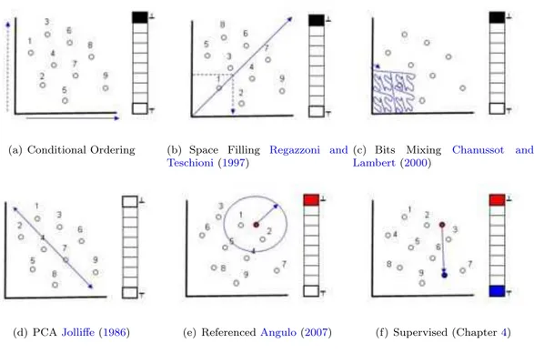
(a) What is a natural order for

these points (in R2_)? (b) Classical approach vector or-_{dering according to a component.}

In this example the x-axis.

(c) Suppose that we know which is the greatest point. Can we order the rest?

(d) Suppose that we know which point are the greatest (top) and the least (bottom). Can we order the rest?

(e) Assume that we have a subset of points as top and bottom points. Can we order the rest?

(f) Can we order the points accord-ing to a measure of outlierness?

Figure 1.10: Different ordering strategies which are discussed in the PartI of this thesis: (c) Refer-enced Ordering (d) Supervised Ordering (e) Supervised Ordering and (f) Unsupervised ordering.

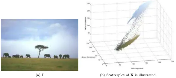
(a) I (b) Scatterplot of X is illustrated.

Figure 1.11: Representation of colour values of natural images as vector points in R3_{. X represents}

pixel values of the image I. Color information are included in the scatterplot to aid the comprehen-sion.

1.5. THESIS OVERVIEW AND MAIN CONTRIBUTIONS ₂₇

(a) Dilation: δSE(I) (b) Erosion: εSE(I)

Figure 1.12: Basic Morphological Transformation obtained by proposed unsupervised ordering (Chapter6).

• Chapter 5 analyses the potential of supervised ordering in morphological template matching

problems, which corresponds to the extension of hit-or-miss operator to multivariate image by using supervised ordering.

• Chapter6proposes methods for unsupervised ordering based on statistical depth function com-puted by random projections. We begin by exploring the properties that we will require our im-age to ensure that the ordering and the associated morphological operators can be interpreted in a similar way to grey scale images. This will lead us to the notion of background/foreground decomposition. Additionally, invariance properties are analysed and theoretical convergence is showed.

PartIIwe present other contributions on mathematical morphology for the analysis of multivariate images.

• Chapter7discusses various strategies for morphological image decomposition, specifically, the additive morphological decomposition is introduced as an alternative for the analysis of remote sensing multivariate images, in particular for the task of supervised/unsupervised classification of hyperspectral remote sensing images.

• That includes also Tensor modelling as an alternative to dimensional reduction approach in multivariate images, by including this step in the traditional pipeline to analysis a hyperspectral image.

• Chapter 8 shifts the focus of our research to conditional morphology as an unified low

com-plexity framework for enhancement and impulse noise removal. Theoretical properties of con-ditional morphology are discussed and applications are widely studied.

• Chapter 9 introduces a new framework of multivariate Boolean models using a complete

lat-tice formulation. This theoretical contribution is useful for characterising and simulation of multivariate textures.

We conclude with a summary of our findings, discussion of ongoing work, and directions for future research in Chapter10. This thesis is the culmination of a variety of intensive collaborations. Most of results have been already published, the first page of each chapter provides the associated references.

Part I

Learning Ordering for Multivariate

Mathematical Morphology

2

Short review on morphological operators for scalar

images

As morphology deals with forms and relations of position, it demands a careful selection of terms, and a methodized nomenclature.

The Anatomical Memoirs of John Goodsir (Volume 2) Chapter V (pp. 83Ð84) Edinburgh, Scotland. 1868

Résumé

Ce chapitre donne un compendium des principaux opérateurs de morphologie mathématique utilisés au cours de la thèse. Les résultats son illustrés au travers d’exemples d’images en niveaux de gris provenant de la télédétection.

2.1

Introduction

Mathematical morphology is a mathematical theory of image processing which facilitates the quan-titative analysis and description of the geometric structures of image. Mathematical morphology discuss nonlinear image transformations such as erosion, dilation, opening, closing, leveling and wa-tershed transformations. In more general scenarios, morphological operators needs a complete lattice structure, i.e., the possibility of defining an ordering relationship between the points to be processed

Ronse (1990b),Goutsias and Heijmans (2000). This key point has been introduced by Jean Serra inSerra(1982) is analysed in Chapter3. The aim of this chapter is to provide a background on the basic morphological operators for scalar images (grey scale images). This short review is necessary to fix the notation and to make easier the definition of the operators for images valued on Rd_.

2.2

Scalar images

Let E be a subset of the Euclidean Rn _{or the discrete space Z}n_{, considered as the support space of}

the image, and let T be a set of grey-levels, corresponding to the space of values of the image. It is 31

32 CHAPTER 2. SHORT REVIEW ON MORPHOLOGICAL OPERATORS assumed that T = R = R [ {−1, +1}. A grey-level image is represented by a function,

I:

⇢ _E

! T

x 7! t (2.1)

i.e., I 2 F(E, T ), where F(E, T ) denotes the functions from the discrete support E onto the space of values of the image T . Thus, I maps each pixel x 2 E into a grey-level value t 2 T : t = I(x). Note that T with the natural order relation  is a complete lattice. It is important to remark that if the T is a complete lattice, then F(E, T ) is a complete lattice too (Serra(1988)).

2.3

Morphological transformations

2.3.1

Dilation and erosion

The two basic morphological mappings F(E, T ) ! F(E, T ) are the level dilation and the grey-level erosion given respectively by

δb(I)(x) = sup h2E(I(x − h) + b(h)) (2.2) and "b(I)(x) = inf h2E(I(x + h) − b(h)) , (2.3)

where I 2 F(E, T ) is the original grey-level image and b 2 F(E, T ) is the fixed structuring function. The further convention to avoid ambiguous expression is considered: I(x − h) + b(h) = −1 when I(x − h) = −1 or b(h) = −1, and that I(x + h) − b(h) = +1 when I(x + h) = +1 or b(h) = −1. Particularly interesting in theory and in practical applications, the flat grey-level dilation and erosion is obtained when the structuring function is flat and becomes a structuring element (Soille(2003)). More precisely, a flat structuring function of the set SE is defined as

b_{(x) =} ⇢

0 x 2 SE

−1 x 2 SEc ,

where SE is a set which indicator function os a Boolean set, i.e., SE ✓ E or SE 2 P(E), which defines the “shape” of the structuring element. We notice that SEc _{denotes the complement set of SE (i.e.,}

SE\ SEc _{= ; and SE [ SE}c _{= E). The structuring element is defined at the origin y 2 E, then to}

each point z of E corresponds the translation mapping y to z, and this translation maps SE onto SE

z, i.e., SEz = {y + z : y 2 SE}. Therefore, the flat grey-level image dilated I(x) with respect to

the structuring element SE is

δSE(I)(x) = sup

h2SE

(I(x − h)) (2.4)

= {I(y) | I(y) = sup[I(z)], z 2 SEx}

and respectively the flat grey-level erosion of a image "SE(I)(x) = inf

h2SE(I(x + h)) (2.5)

= {I(y) | I(y) = inf[I(z)], z 2 ˇSE_x},

where ˇSEis the reflection of SE with respect to the origin, i.e., ˇSE_{= {−b | b 2 SE}. Dilation and} erosion are dual operators with respect to the image complement (negative), i.e.,

δSE(I) = ("SEˇ(Ic))c

where Ic_{(x) = −I(x). Dilation and erosion are increasing operators: if I(x)  J(x), 8x 2 E, then}

δSE(I)  δSE(J) and "SE(I)  "SE(J), 8x 2 E. Dilation (erosion) is an extensive (anti-extensive)

2.3. MORPHOLOGICAL TRANSFORMATIONS ₃₃

Dilation and erosion are also negative operators in the following sense: (δSE(I))c= "SEˇ(Ic)

This means that dilation of the image foreground has the same effect as erosion of the background (with the reflected structuring element). However, the heart of the construction of the morphological operators is the duality in the adjunction sense, namely

δSE(J)  I () J  "SE(I) (2.6)

for every pair of images I, J 2 F(E, T ). This is called the adjunction relation forms the basis of the extension of mathematical morphology to complete lattice Serra (1982), Heijmans(1995). An important point is that given an adjunction ("SE(·) , δSE(·)), then "SE(·) is an erosion (it distributes

over infimum) and δSE(·) is a dilation (it distributes over supremum). Additionally, the two following

properties also hold: • Distributivity:

δSE(I _ J) (x) = δSE(J) (x) _ δSE(I) (x)

"SE(I ^ J) (x) = "SE(I) (x) ^ "SE(J) (x)

• Associativity:

δSE_1⊕SE2(δSE₃(I))(x) = δSE₁(δSE_2⊕SE3(I))(x)

where SE1⊕ SE2 is the Minkowski addition of the structuring elements. Fig. 2.1 shows the effect

of these operators for a real high-resolution remote sensing image. These two elementary operators can be viewed as building blocks of more advanced morphological operators.

2.3.2

Opening and closing

The two elementary operations of grey-level erosion and dilation can be composed together to yield a new set of grey-level operators having desirable feature extractor properties which are the opening and the closing. More precisely, starting from the adjunction pair {"b(·), δb(·)}, the opening and

closing of a grey-level image Iaccording to the structuring function b are the mappings F(E, T ) ! F(E, T ) given respectively by

γb(I)(x) = δb("b(I))(x), (2.7)

and

'b(I)(x) = "b(δb(I))(x). (2.8)

The flat counterparts are obtained by using the flat erosion and flat dilation by the structuring element SE. The opening and closing are dual operators, i.e.,

γSE(I) = ('SE(Ic))c

Opening (closing) removes positive (negative) structures according to the predefined size and shape criterion of the structuring element SE: they smooth in a nonlinear way the image.

The pair (γSE(·), 'SE(·)) is called adjunction opening and adjunction closing. Let I, J 2 F(E, T )

be two grey-level images. The opening γSE(·) and closing 'SE(·) verify the following properties.

• Increasingness (ordering preservation): γSE(·) and 'SE(·) are increasing as products of increasing

operators, i.e., I(x)  J(x) ) γSE(I)(x)  γSE(J)(x), 'SE(I)(x)  'SE(J)(x).

• Idempotence (invariance with respect to the transformation itself): γSE(·) and 'SE(·) are

idem-potent, i.e., γSE(γSE(I)) = γSE(I), 'SE('SE(I)) = 'SE(I).

• Extensivity and anti-extensivity: γSE(·) is anti-extensive, i.e., γSE(I)(x)  I(x); and 'SE(·) is

extensive, i.e., I(x)  'SE(I)(x).

Examples of opening/closing in a high-resolution remote sensing image are illustrated in Fig. 2.2. The other morphological operators are obtained as products of openings/closings or by residues between erosion/dilation and opening/closing.

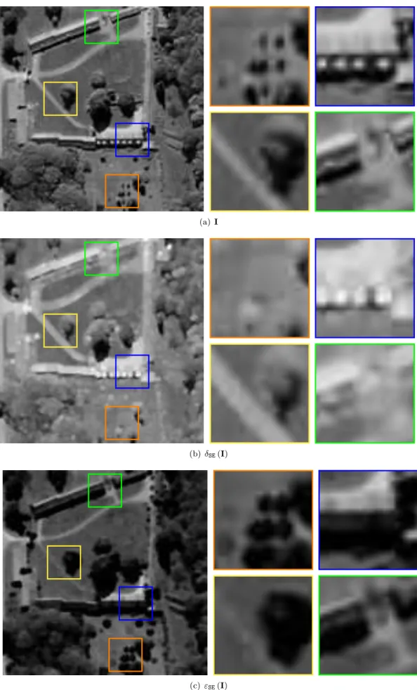
34 CHAPTER 2. SHORT REVIEW ON MORPHOLOGICAL OPERATORS

(a) I

(b) δSE(I)

(c) εSE(I)

Figure 2.1: Basic morphological transformations: dilation (b) and erosion (c). The structuring element SE is a disk of diameter three pixels.

2.3. MORPHOLOGICAL TRANSFORMATIONS ₃₅

(a) γSE(I)

(b) ϕSE(I)

Figure 2.2: Opening (a) and closing (b) transformations. The structuring element SE is a disk of diameter 3 pixels.

36 CHAPTER 2. SHORT REVIEW ON MORPHOLOGICAL OPERATORS

2.3.3

Contrast mappings

The contrast mapping is a particular operator from a more general class of transformations called toggle mappings Serra(1989b). A contrast mapping is defined, on the one hand, by two primitives Φ1and Φ2 applied to the initial function, and on the other hand, by a decision rule which makes, at

each point x the output of this mapping toggles between the value of Φ1 at x and the value of Φ2,

according to which is closer to the input value of the function at x. ⌧(Φ1,Φ2)(I)(x) =

⇢

Φ2(I)(x) if kI(x) − Φ2(I)(x)k  kI(x) − Φ1(I)(x)k

Φ1(I)(x) if kI(x) − Φ2(I)(x)k > kI(x) − Φ1(I)(x)k (2.9)

If the pair of primitives (Φ1(I), Φ2(I)) are an erosion "SE(I) and the adjunction dilation δSE(I),

the toggle mapping for an image I is given byKramer and Bruckner(1975): ⌧("SE(·),δSE(·)):= ⌧ (I)(x) =

⇢

δSE(I) (x) if kI(x) − δSE(I) (x)k  kI(x) − "SE(I) (x)k

"SE(I) (x) if kI(x) − δSE(I) (x)k > kI(x) − "SE(I) (x)k

(2.10) where δSE(I) and "SE(I) are dilation and erosion transformations and the norm are differences in

grey scale values. This morphological transformation enhances the local contrast of I by sharpening its edges. It is usually applied more than once, being iterated, and the iterations converge to a limit reached after a finite number of iterations, because we only consider the case of images with

finite support. An example is shown in Fig. 2.3. Another interesting contrast mapping is defined

by changing the previous expression for the pair of opening γSE(I) and its dual closing 'SE(I)Meyer

and Serra(1989).

2.3.4

Morphological center

The opening/closing are nonlinear smoothing filters, and classically an opening followed by a closing (or a closing followed by an opening) can be used to suppress impulse noise, i.e., suppressing posi-tive spikes via the opening and negaposi-tive spikes via the closing and without blurring the contours. A more interesting operator to suppress noise is the morphological center, also known as automedian filterSerra(1982, 1989b). Given an opening γSE(I) and the dual closing 'SE(I) with a small

struc-turing element (typically a discrete disk of diameter equal to the “noise scale”), the morphological center associated to these primitives for an image I is given by the algorithm:

⇣(I) = [I _ (γSE('SE(γSE(I))) ^ 'SE(γSE('SE(I))))] ^ (γSE('SE(γSE(I))) _ 'SE(γSE('SE(I))). (2.11)

This is an increasing and autodual operator, not idempotent, but the iteration of ⇣(·) presents a point monotonicity and converges to the idempotence, i.e. d⇣(I) = [⇣(I)]i_{, such that [⇣(·)]}i_{= [⇣(·)]}i+1_.

An example of this filter is illustrated in Fig. 2.3.

2.3.5

Geodesic reconstruction, derived operators, leveling

The geodesic dilation is based on restricting the iterative unitary dilation of an image M 2 F(E, T ) called function marker by an isotropic structuring element associated with the smallest connectivity (a disk of diameter three for 4-connectivity or a square of side three for 8-connectivity, see Fig. 1.7), denoted by B, to a function reference IVincent(1993), i.e.,

δi

B(I, M) = δ 1

B(δBi−1(I, M)), (2.12)

where the unitary dilation controlled by I is given by δ1

B(I, M) = δB(M) ^ I. The reconstruction by

dilation is then defined by

δB1(I, M) = δ i B(I, M), (2.13) such that δi B(I, M) = δ i+1 B (I, M) (idempotence).

Equivalently, geodesic erosion is defined as follows "iB(I, M) = "

1 B("

i+1

2.3. MORPHOLOGICAL TRANSFORMATIONS ₃₇

(a) τ (I)

(b) ζ(I)

Figure 2.3: Results of toggle mapping and morphological center. In both cases, the structuring element SE is a digital disk of diameter three pixels.

38 CHAPTER 2. SHORT REVIEW ON MORPHOLOGICAL OPERATORS

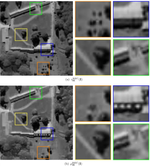
(a) γREC SE (I)

(b) ϕREC SE (I)

Figure 2.4: Opening (a) and closing (b) by reconstructions, where the markers are respectively the opening and closing adjunction of Fig. 2.2.

2.3. MORPHOLOGICAL TRANSFORMATIONS ₃₉

where the unitary dilation controlled by I is given by "1

B(I, M) = "B(M) _ I. The reconstruction by

erosion is then defined by

"1B (I, M) = " i B(I, M), (2.15) such that "i B(I, M) = " i+1

B (I, M) (idempotence). The important issue at this point is how to select

an adequate image marker M.

Opening/Closing by reconstruction

The opening by reconstruction is a geodesic reconstruction by using an opening as marker, i.e., γRECSE (I) := γ

REC

SE (I, γSE(I)) = δB1(I, γSE(I)) (2.16)

γSE(I) (from an erosion/dilation) modifies the contours, the opening by reconstruction γ REC SE (I) is

aimed at efficiently and precisely reconstructing the contours of the objects which have not been totally removed by the marker filtering process. Accordingly the closing by reconstruction 'REC

SE (I)

is a erosion by reconstruction by using a closing as marker. Comparison of both morphological transformations is shown in Fig. 2.4.

Leveling

In a similar way, the leveling Λ(I, M) of a reference function I and a marker function M is a symmetric geodesic operator computed by means of an iterative algorithm with geodesic dilations and geodesic erosions until idempotenceMeyer (1998), i.e.

Λi_{(I, M) =}⇥_{I^ δ}i B(M)

⇤ _ "i

B(M), (2.17)

until Λi_{(I, M) = Λ}i+1_{(I, M). The leveling simplifies the image, removing the objects and textures}

smaller than the structuring element and preserving the contours of the remaining objects. Moreover, it acts simultaneously on the “bright” and “dark” objects. The usefulness of this transformation is related to the role of the marker image M. Different types of markers have been considered in the literature, for instance, Alternate Sequential Filter, Isotropic Gaussian Function or Anisotropy diffusion filtering. Figs. 2.5 and2.6illustrate two different markers and the correspondent leveling operator.

2.3.6

Residue-based operators

From definition of basic morphological operators is easy to define the morphological gradient

∆SE(I) := δSE(I) − "SE(I) (2.18)

The structuring element SE for the gradient is generally the unitary ball B. This function gives the contours of the image, attributing more importance to the transitions between regions close/far to the background/foreground. Similarly, the positive(white) top-hat transformation is the residue of an opening, i.e.,

⇢+SE(I) = I − γSE(I). (2.19)

Dually, negative(black) top-hat transformation is given by

⇢−SE(I) = 'SE(I) − I. (2.20)

The top-hat transformation yields grey level images and is used to extract contrasted components. Moreover, top-hats remove the slow trends, and thus enhancing the contrast of objects smaller than the structuring element SE used for the opening/closing.

40 CHAPTER 2. SHORT REVIEW ON MORPHOLOGICAL OPERATORS

(a) γSE(ϕSE(I))

(b) Λ(I, γSE(ϕSE(I)))

2.3. MORPHOLOGICAL TRANSFORMATIONS ₄₁

(a) σ ∗ I

(b) Λ(I, σ ∗ I)

42 CHAPTER 2. SHORT REVIEW ON MORPHOLOGICAL OPERATORS (a) ∆SE(I) (b) ∆δ SE(I) (c) ∆" SE(I)

Figure 2.7: Morphological gradients: (a) symmetric gradient, (b) gradient by dilation (∆δ SE(I) =

2.4. MORPHOLOGICAL SEGMENTATION ₄₃

2.4

Morphological Segmentation

For grey scale images, the watershed transform, originally proposed byLantuéjoul(1978) and later

improved by Beucher and Lantuejoul (1979), is a region based image segmentation Beucher and

Meyer (1993). Works on watersheds began over a hundred years ago when Cayley and Maxwell (Cayley (1859), Maxwell (1870)), described how smooth surfaces could be decomposed into hills and dales by studying the critical points and slope lines of a surface. The intuitive idea underlying this method comes from geography: it is that of a landscape or topographic relief which is flooded by water, watersheds being the divide lines of the domains of attraction of rain falling over the region. The watershed algorithm Vincent and Soille (1991) is a flooding process: water, starting from specified markers, “floods" the image, from the smallest to highest grey values. When two catchment basins meet, a dam is created, called “watershed plane". This presentation is called the “flooding paradigm". However, there exist many possibles way to defining a watershedNajman and Schmitt(1994),Roerdink and Meijster(2000),Bertrand(2005),Cousty et al.(2009),Meyer(2012).

Additionally, random marker process have been introduced in Angulo and Jeulin (2007) to yield

a stochastic watershed that can be interpreted as to give an edge probability for a given image. Recently, links between watershed algorithm as a Maximum a Posteriori estimation of a Markov Random Field have been introduced inCouprie et al.(2011).

In this document, we denote the watershed transformation of an image M, by using a set the markers

M (seeds in the flooding process) as WS(I, M). Watershed transformation is typically applied on

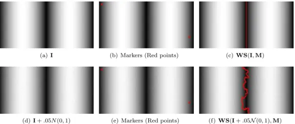
the gradient magnitude image, i.e., the morphological gradient. A simple example of the watershed with two markers is illustrated in Fig. 2.8. We can observe that watershed is relatively sensitive to noise. Over-segmentation is a well-known difficulty with this approach, which has led to a number of approaches for merging watershed regions to obtain larger regions corresponding to objects of interestBeucher and Meyer(1993),Gauch (1999),Cousty et al.(2010),Najman (2011). A simple approach to deal with the over-segmentation problem consists in determine markers for each region of interest, for instance, the dynamics or contrast based transform applied to the minima of the gradient image. The parameter t in the contrast based transform, is normalized to (0, 1) with respect to the minimum and maximum of the original image. We denote this approach as WS(I, t) for some parameter t 2 (0, 1). Note that WS(I, 0) = WS(I). Watershed regions associated with different value of t are illustrated for the same original image (see Fig. 2.9). From this example, we observe that different levels of segmentation with respect to t constitute a hierarchical (pyramid) of regions. Watershed transform have been applied in multidimensional remote sensing application, where the important selection of an adequate multivariate gradient is still an open problemNoyel et al.(2007),Tarabalka et al.(2010b).

44 CHAPTER 2. SHORT REVIEW ON MORPHOLOGICAL OPERATORS

(a) I (b) Markers (Red points) (c) WS(I, M)

(d) I + .05N (0, 1) (e) Markers (Red points) (f) WS(I + .05N (0, 1), M)

Figure 2.8: Watershed transform for a given image I, with markers point M are the red points in (b) and (e). (Watershed Transform is applied in ∆SE(I)).

2.4. MORPHOLOGICAL SEGMENTATION ₄₅

(a) WS(I, .01)

(b) WS(I, .06)

46 CHAPTER 2. SHORT REVIEW ON MORPHOLOGICAL OPERATORS

(d) WS(I, .16)

(e) WS(I, .21)

(f) WS(I, .26)

Figure 2.9: Contrast-driven watershed transforms with markers calculated as % of the maximum value in I.

3

Preliminary Notions

By a tranquil mind I mean nothing else than a mind well ordered. Marcus Aurelius

Résumé

Ce chapitre donne un présentation générale de la représentation spectrale d’une image multivariée. Pour le cas particulier de la représentation basée sur un ordre total, l’ordre-h est utilisé pour ap-préhender le caractère vectoriel des images multidimensionnelles. Les aspects les plus importants de la théorie des treillis liés à cette thèse sont présentés en détail.

3.1

Introduction

Digital image processing is an expanding and dynamic area with applications reaching out into our everyday life as surveillance, medicine, authentication, automated industrial quality control and many more areas. An important research topic is to design parameter-free algorithms or at least approaches where the parameter model can be interpreted in the context of the problem. However, on the one hand, a parameter-free algorithm would limit our ability to impose our prejudices, expectations, presumptions, or any a priori information on the problem setting. On the other hand, an incorrect setting in a non-parameter free approach may cause that an algorithm to fail in finding the true patterns. A useful approach to tackle this kind of problems for image processing is mathematical morphology. It consists of a set of operators that transform image according to geometric characteristics as size, shape, connectivity, etc. Serra (1982). In this chapter we review some results related to mathematical morphology for multivariate images, i.e., in each pixel of the image a vector information is available. We include several results of flat operator for images

I : E ! L, where L is a lattice of values. Details about lattice formulation and mathematical

morphology can be found in e.g. Ronse (2006) and Chapter 2 (J. Serra and C. Ronse) in Najman

and Talbot(2010). Most morphological operators used for processing and filtering are flat operators. This means that they are grey-level extensions of the operators for binary images, and they can be obtained bySerra(1982):

1. thresholding the grey-level image for all values of the image, 2. applying the binary operator to each thresholded image set, 3. superposing the resulting set.