Laboratoire d'Analyse et Modélisation de Systèmes pour l'Aide à la Décision CNRS UMR 7024
CAHIER DU LAMSADE
226
Septembre 2005Approximate solutions of HAPPYNET on cubic graphs Aristotelis Giannakos, Olivier Pottie
Approximate solutions of H
APPYNET
on cubic
graphs
Aristotelis Giannakos
∗, Olivier Pottié
†Abstract
The HAPPYNETproblem is defined as follows : Given a undirected simple graph G with integer weights wvuon its edges vu ∈ E(G), find a function s : V (G) −→
{−1, 1} such that ∀v ∈ V (G), v is happy in G, i.e. such thatPu∈Γ(v)s(v)s(u)wuv≥
0. It is easy to see [3] that HAPPYNEThas always a solution, no matter what the input
is. However, no polynomial algorithm is known for this problem, which is complete for the class PLS (see [4] for a definition). Parberry et al. have shown in [7] that in the case of cubic graphs (i.e. of maximum degree 3) HAPPYNETis as difficult as for arbitrary graphs. A ρ-approximate solution to a HAPPYNETinstance of size n can be defined for 0 ≤ ρ ≤ 1 as a natural extension of the solution function, with at least ρn happy vertices. In this paper, we present a polynomial-time algorithm that finds a ρ-approximate solution for the HAPPYNETproblem on cubic graphs, with ρ ≥ 34.
1
Introduction
All graphs G considered throughout this paper are finite, undirected simple graphs. As usually, we denote by V (G) (resp., E(G)) the set of vertices (resp., edges) of G and n (resp., m) its cardinality. An edge between a vertex u and a vertex v is denoted by uv or
vu, without any distinction.
The HAPPYNETproblem can be defined as follows :
INPUT: G a graph with integer weights wuvon its edges uv. OUTPUT: A function s of the vertices of G to {−1, 1} such that
∗LAMSADE, Université Paris-Dauphine, 75775 Paris cedex 16, France. {giannako,
∀v ∈ V (G), X
uv∈E(G)
s(u)s(v)wuv ≥ 0 (1)
HAPPYNET is in fact the problem of finding a stable state in a symmetric Hopfield
network, first considered in [2], restricted to the case where the threshold of every vertex
is equal to zero. There are several equivalent formulations of HAPPYNET , in terms of fixed-point searching (given a symmetric integer matrix W with a zero diagonal, find a fixed-point of the mapping x 7→ sgn(W x), from {−1, 1}n into itself) or game theory; elegant geometric formulations can be found as well.
Complexity results for HAPPYNETwere first given in [1]. A simple argument [3] can show that there is always a solution for HAPPYNET, no matter what the input is: consider an input graph G, an arbitrary total function s from the vertices of G to {−1, 1}, and the corresponding sum of s(u)s(v)wuv over all edges uv of G, which is always bounded by the sum of absolute values of the weights. Notice that if there is a vertex v such thatX vu∈E(G)
s(v)s(u)wuv < 0, then the function s0with s0(w) = s(w) if w 6= v, s0(v) = −s(v) corresponds to X uv∈E(G) s0(u)s0(v)w uv> X uv∈E(G)
s(u)s(v)wuv, meaning that after successive transformations of s a solution will always be finally obtained.
Unfortunately, the algorithm suggested above may not be polynomial on n.
The function s can also be interpreted as a vector in {−1, 1}n and the HAPPYNET problem as the search of a local optimum for the cost function
X
uv∈E(G)
s(u)s(v)wuv in the solution space SG made of all s-vectors, where two vectors are considered as neighbors iff their Hamming distance is one.
Thus, HAPPYNETbelongs to the class PLS first defined in [4]. In [6] the HAPPYNET problem is shown to be complete for this class.
A natural problem is then to define in polynomial time a function s that satisfies
X
uv∈E(G)
s(u)s(v)wuv ≥ 0 for “as many as possible” vertices v of the input graph. This problem can be seen as an optimization version of HAPPYNET , when polynomial-time constraints are applied to the search for a solution.
In this paper, we deal with this above-mentionned version of HAPPYNET i.e. with searching in polynomial time for functions s such that for each vertex v of at least ρn vertices of the input, 0 ≤ ρ ≤ 1, we have
X
vu∈E(G)
s(v)s(u)wvu ≥ 0.
In the rest of this section, formal definitions are given, and a result of Parberry and Tseng [7], showing the PLS-completeness of HAPPYNETfor cubic graphs is recalled. In
and one with ρ ≥ 34 for cubic graphs. Finally, in the last section, some open questions are briefly discussed.
1.1
Notations and preliminaries
Let G0be a subgraph of G, i.e. such that V (G0) ⊆ V (G) and E(G0) ⊆ E(G)∩V (G0)×
V (G0). The set of neighbors of a vertex v of G in G0, i.e. the set {u ∈ V (G)|vu ∈ E(G0)} is noted ΓG0(v) and its size |ΓG0(v)|. The degree of v in G0is noted dG0(v); when G0 = G, we will simply note Γ and d(v) without any risk of confusion.
Let G be a graph with integer-weighted edges. Any function s : V (G) −→ {−1, 1} will be called a partial solution (for HAPPYNET) on G; s(v) will be called the state of v within s. The set of all the partial solutions on G will be denoted by SG.
The function H : SG× V (G) −→ Z with H(s; v) =
X
u∈Γ(v)
s(u)s(v)wuv is called the
happiness of v in G with s; the sign of H(s; v) will be called the happiness state of v with
s and will be noted h(s; v); if h(s; v) = 1 (resp. -1) then v will be said to be happy (resp.
unhappy) with s.
A partial solution is called ρ-approximate if 1
2n X
v∈V (G)
(1 + h(s; v)) ≥ ρ. A total
solution (or simply a solution) is a 1-approximate solution.
Let s be a partial solution on G, and let A ⊆ V (G). We note s[A, −A], a new partial solution s0 on G obtained by flipping (reversing) in s the states of the vertices of A:
s0(v) = −s(v) if v ∈ A, s0(v) = s(v) otherwise; if A is a singleton, the hooks will be omitted. Obviously, for every partial solution s ∈ S on G, and for every vertex in V (G), we have H(s; v) = H(s[V (G), −V (G)]; v).
An edge uv in G is called strong (resp. weak) with s, if s(u)s(v)wuv≥ 0 (resp. < 0). A vertex v is called strongly happy in G with s, if for all of its neighbors u the edge
vu is strong with s.
A solution s is called strong in G if every vertex of the input graph G is strongly happy with s.
It can be shown directly from the results of Parberry et al. in [7] that HAPPYNETon cubic graphs remains PLS-complete, as for general graphs.
2
H
APPYNET
on cubic graphs
Proposition 1 1 Let G be a connected graph. Then G has always a solution which is a
strong solution for some spanning tree of G.
Proof :
Consider a solution sG : obviously, for every vertex v of the graph there is a strong edge vu. Thus the strong edges with sGinduce a spanning subgraph Gsσ of G.
By the construction, the edges of G between connected components of Gsσ are weak. Furthermore, if Ci is such a component, then with s0 = s[V (Ci), −V (Ci)] all the edges of G between V (Ci) and V (G) \ V (Ci) become strong, while all the other edges of G remain as they were in s.
So the spanning subgraph Gsσ0 will contain less connected components than Gsσ. Ap-plying successively n times the same procedure, will yield a solution sT where the span-ning subgraph of strong edges is connected, i.e. such that sT is a strong solution for some spanning tree of G. ¤ + - -+ + + + + + + C3 C2 C1 + + -+ + + + + + + C3 C2 C1 + -+ + + + + + + C2 C1 + A B C
Figure 1: Illustration of Proposition 1. In A, C1, C2, C3 are connected components in-duced by strong edges in a solution (those labelled with a “+”). White and black vertices are in opposite states. Flipping the states of the vertices in C1, as shown in B, just changes the edges connecting C1 to the rest of the graph from weak to strong; thus in the obtained solution, C1 and C2 have been merged (C).
Corollary 1 There is always a strong solution for HAPPYNETon a tree.
Corollary 1 can also be seen as a consequence of the following proposition:
Proposition 2 Let G1, G2 be two graphs such that |V (G1) ∩ V (G2)| = 1, and s1 (resp.,
s2) a ρ-approximate solution for G1 (resp., G2). Then there exists an efficient algorithm
for finding an approximate solution for G = (V (G1) ∪ V (G2), E(G1) ∪ E(G2)) of ratio
ρ0, where ρ0 ≥ ρ¡1 + 1
|V (G)|
¢
− 1
Let p be the vertex that G1 and G2 have in common. Then s1(p) is equal to either
s2(p) or s02(p) where s02 = s2[V (G2), −V (G2)] which are both ρ-approximate; w.l.o.g.,
let s1(p) = s2(p).
Consider s defined in G by the union of s1and s2:
∀v ∈ V (G1), s(v) = s1(v) and ∀v ∈ V (G2), s(v) = s2(v). Now, if p is happy in s1, and
in s2, or it is happy only in one of them but unhappy in s, we have ρ0 = ρ −
1 − ρ |V (G)| = ρ¡1 + 1 |V (G)| ¢ − 1
|V (G)|, otherwise (if p is unhappy in both s1 and s2, or it is happy in
only one of them but happy in s) we have ρ0 = ρ¡1 + 1
|V (G)|
¢ ¤
Hence it is possible to find a strong solution for a tree by finding a strong solution for every edge and combining them as suggested above. Furthermore, the same method can be applied when (total) solutions are given for the biconnected components of a graph; so the following corollary is straightforward :
Corollary 2 Finding a total solution for HAPPYNETon biconnected graphs is as difficult as solving HAPPYNETon general graphs.
2.1
An algorithm for finding a strong solution on a tree
However, finding a strong solution on a tree can be easier than combining strong solutions on every edge as suggested above : in fact, finding the states of a strong solution can be done with any BFS- or DFS-like traversal of the tree, as shown by algorithm A presented below :
Algorithm A
Input : A tree T with integer weights on its edges. Output : A strong solution s for T .
PROCEDURE Visit_and_Solve(x:vertex) BEGIN /*Visit_and_Solve*/
Mark x as visited
Let p be the parent of x: /*r begin the parent of itself*/ s(x) <- s(p)*sgn(w[p,x]) /*w[p,x] is the weight of the edge px*/ FOR all unvisited children of x:
Visit_and_Solve(y) ENDFOR
END /*Visit_and_Solve*/ BEGIN /*Main*/
FOR all vertices v of T: s(v) <- 1
Mark v as unvisited ENDFOR
Pick at random a vertex r and root T at r Visit_and_Solve(r)
Return(s) END /*Main*/
Theorem 1 Algorithm A correctly computes a strong solution for HAPPYNETon a tree.
Proof : By induction on the number of vertices of the tree: for n = 2 the statement
is trivial. Observe that the last vertex v to be marked as visited is a leaf of the tree; so assuming that A computes a strong solution for any tree of size ≤ n, in order to prove that it does so for any tree of size n + 1, it suffices to show that the edge pv connecting the last visited vertex v to the tree is strong; indeed, we always have s(p)sgn(wpv)s(v) =
s(p)2sgn(w
pv)2 = 1 ¤
2.2
A tree-based algorithm for finding a ρ-approximate solution
Proposition 1 provides the central idea behind the algorithm discussed in the rest of this paper, that is, to find first a strong solution for some spanning subgraph, when it is possible to do so, and then to improve the partial solution obtained for the graph by flipping the states of some carefully chosen vertices. Obviously, algorithm A runs in polynomial time.
Input : A graph G of maximum degree 3 with integer weights on its edges. Output : A ρ-approximate solution s for G.
PROCEDURE Improvement_Step(s:solution, T:tree) BEGIN /* Improvement_Step */
WHILE there exist edges vu,uw of G with u,v,w leaves of T unhappy in G: s <- s[u,-u] /* Phase 1: flip the state of u */
ENDWHILE
WHILE there exist edges vu of G with v,u leaves of T unhappy in G: s <- s[v,-v] /* Phase 2: flip the state of v */
ENDWHILE
FOR each remaining leaf v of T unhappy in G:
IF v has a sibling u THEN /* Phase 3: flip the state of leaves with siblings */ s <- s’ where s’ is the one of s[v,-v], s[u,-u], having the greatest
number of happy vertices with it in G ENDIF
IF s[v,-v] has more happy vertices (in G) than s THEN s <- s[v,-v]
ENDIF ENDFOR
END /* Improvement_Step */ BEGIN /* Main */
Compute a maximum absolute weight spanning tree T_max_abs of G Run A on T, that is T_max_abs with the edges weights signed as in G Improvement_Step(s,T)
Return(s) END /* Main */
It is straightforward that algorithm B runs in polynomial time.
Notice also that algorithm B finds a total solution for graphs of degree 2, i.e. for systems of cycles and paths.
Hence, the following theorem holds :
Theorem 2 Algorithm B when applied on cubic integer-weighted graphs computes a
ρ-approximate solution with ρ = 3
4.
Proof :
The two following remarks are important :
1 Just before the execution of the improvement step, only tree leaves of degree three
2 After the execution of the improvement step, the number of vertices unhappy with
the computed solution is bounded by the number of parents of the unhappy vertices before the improvement step.
Furthermore, the maximum number of parents of leaves v with dG(v) = 3 is less or equal to 1
4 of the set of vertices of the graph. The proof is now straightfoward ¤
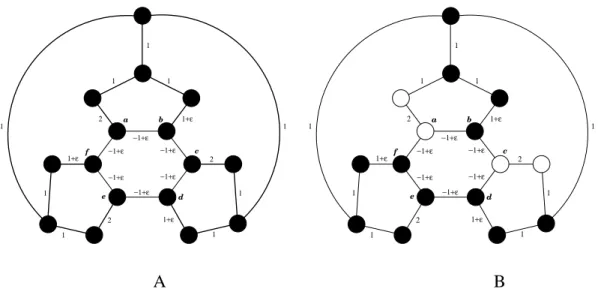
1+ε 1 −1+ε 2 1 1 −1+ε −1+ε −1+ε −1+ε −1+ε 1+ε b c 1 d f a e 2 1+ε 1 1 2 1 1 1 1+ε 1 −1+ε 2 1 1 −1+ε −1+ε −1+ε −1+ε −1+ε 1+ε b c 1 d f a e 2 1+ε 1 1 2 1 1 1 A B
Figure 2: An instance where algorithm B performs as badly as possible when 0 < ² < 13. On the left (A), the solution computed by B : all vertices are in the same state. The edges of the maximum absolute weight spanning tree are drawn thick; b, d and f are unhappy with the cmputed solution (i.e. ρ = 1316 on this instance). On the right (B), a total solution for the same instance is shown; black and white vertices are in opposite states.
3
Open questions and perspectives
Certainly, solving exactly in polynomial time a PLS-complete problem should imply the existence of powerful general-purpose methods for finding local optima, at a level of sophistication comparable to the elipsoid or Karmakar’s algorithm for linear programming [6]. However, the search for algorithms that obtain partial (i.e. approximate) solutions to such problems may give useful insight about the structure and distribution of local optima. We have conjectured, without being able to prove it, that algorithm B can give guar-anteed ρ-approximate solutions for HAPPYNETwith ρ = 45.
the input graph into a cubic graph, following the method explained in [7]. We believe that, up to slight modifications, our algorithm can give guaranteed ρ-approximate solutions with ρ > 12 on any input graph whose maximum degree is bounded by a constant.
Another direction for future work could be to construct a more elaborate Improvement Step of our algorithm to “push” the unhappy leaves higher in the tree; also to start with a strong solution on spanning graphs other than the maximum absolute weights spanning tree.
Finally, it could be of interest to evaluate the performance of algorithm B on approx-imating maximum weights cuts on cubic graphs (which can be done by taking as input of B the input graph of the instance of MAXCUT with the corresponding edges weights multiplied by -1).
References
[1] G.H. Godbeer, J. Lipscomb, M. Luby, On the computational complexity of find-ing stable state vectors in connectionist models (Hopfield nets). Technical Report
208/88, Dept. of Computer Science, Univ. of Toronto, 1988.
[2] J.J. Hopfield, Neural networks and physical systems with emergent collective computational activities. In Proc. USA Nat. Ac. Sc, 1982, 30:709-728.
[3] C.H. Papadimitriou, Computational complexity. Addison-Wesley, 1994.
[4] D.S. Johnson, C.H. Papadimitriou, M. Yannakakis, How easy is local search? In
Proc. 26th FOCS, 1985, 39-42.
[5] C.H. Papadimitriou, A. Schäffer, M. Yannakakis, On the complexity of local search. In Proc. 22nd STOC, 1990, 439-445.
[6] A. Schäffer, M. Yannakakis, Simple local search problems that are hard to solve,
SIAM Journal on Computing 20 (1), 1991, 56-87.
[7] I. Parberry, H-L. Tseng, Are Hopfield networks faster than conventional com-puters? In Proc. of the 9th Conference on Neural Information Systems, 1997,