Bootstrap and uniform bounds for Harris Markov chains

(1)

HAL Id: tel-01988595

https://pastel.archives-ouvertes.fr/tel-01988595

Submitted on 21 Jan 2019

HAL is a multi-disciplinary open access

archive for the deposit and dissemination of sci-entific research documents, whether they are pub-lished or not. The documents may come from teaching and research institutions in France or

L’archive ouverte pluridisciplinaire HAL, est destinée au dépôt et à la diffusion de documents scientifiques de niveau recherche, publiés ou non, émanant des établissements d’enseignement et de recherche français ou étrangers, des laboratoires

Bootstrap and uniform bounds for Harris Markov chains

Gabriela Ciolek

To cite this version:

Gabriela Ciolek. Bootstrap and uniform bounds for Harris Markov chains. Statistics [math.ST]. Université Paris-Saclay, 2018. English. �NNT : 2018SACLT024�. �tel-01988595�

(2)

NNT : 2018SACLT024

TH`

ESE DE DOCTORAT

de

l’Universit´

e Paris-Saclay

´

Ecole doctorale de math´ematiques Hadamard (EDMH, ED 574)

´

Etablissement d’inscription : T´el´ecom ParisTech

´

Laboratoire d’accueil : Laboratoire traitement et communication de l’information

Sp´ecialit´e de doctorat :

Math´ematiques appliqu´ees

Gabriela CIO�LEK

Bootstrap and uniform bounds for Harris Markov chains

Date de soutenance : 14 D´ecembre 2018

Apr`es avis des rapporteurs : Kengo KATO (Cornell University)

Olivier WINTENBERGER (Sorbonne Universit´e)

Jury de soutenance :

Patrice BERTAIL (Universit´e Paris Nanterre) Codirecteur de th`ese

Stephan CLÉMENÇ ON (Télécom ParisTech) Codirecteur de thèse

Randal DOUC (T´el´ecom SudParis) Examinateur

C´ecile DUROT (Universit´e Paris Nanterre) Examinateur

Kengo KATO (Cornell University) Rapporteur

Sana LOUHICHI (Universit´e de Grenoble) Pr´esident

(3)

(4)

Titre : Bootstrap et bornes uniformes pour des chaˆınes de Markov Harris récurrentes Mots Clefs : Chaˆınes de Markov, processus régénératifs, bootstrap, robustesse, inégalités de concentration, apprentissage statistique

Résumé : Cette thèse se concentre sur certaines extensions de la théorie des processus empiriques lorsque les données sont Markoviennes. Plus spécifiquement, nous nous con-centrons sur plusieurs développements de la théorie du bootstrap, de la robustesse et de l’apprentissage statistique dans un cadre Markovien Harris récurrent positif. Notre approche repose sur la méthode de régénération qui s’appuie sur la décomposition d’une trajectoire de la chaˆıne de Markov atomique régénérative en blocs d’observations indépendantes et identiquement distribuées (i.i.d.). Les blocs de régénération correspondent à des segments de la trajectoire entre des instants aléatoires de visites dans un ensemble bien choisi (l’atome) formant une séquence de renouvellement. Dans la première partie de la thèse nous propo-sons un théorème fonctionnel de la limite centrale de type bootstrap pour des chaˆınes de Markov Harris récurrentes, d’abord dans le cas de classes de fonctions uniformément bornées puis dans un cadre non borné. Ensuite, nous utilisons les résultats susmentionnés pour ob-tenir un théorème de la limite centrale pour des fonctionnelles Fréchet différentiables dans un cadre Markovien. Motivés par diverses applications, nous discutons la manière d’étendre cer-tains concepts de robustesse à partir du cadre i.i.d. à un cas Markovien. En particulier, nous considérons le cas où les données sont des processus Markoviens déterministes par morceaux. Puis, nous proposons des procédures d’échantillonnage résiduel et wild bootstrap pour les processus périodiquement autorégressifs etétablissons leur validité. Dans la deuxième partie de la thèse, nous établissons des versions maximales d’inégalités de concentration de type Bernstein, Hoeffding et des inégalités de moments polynomiales en fonction des nombres de couverture et des moments des temps de retour et des blocs. Enfin, nous utilisons ces inégalités sur les queues de distributions pour calculer des bornes de généralisation pour une estimation d’ensemble de volumes minimum pour les chaˆınes de Markov régénératives.

(5)

Title : Bootstrap and uniform bounds for Harris Markov chains

Keys words : Markov chains, regenerative processes, bootstrap, robustness, concentration inequalities, statistical learning

Abstract : This thesis concentrates on some extensions of empirical processes theory when the data are Markovian. More specifically, we focus on some developments of bootstrap, ro-bustness and statistical learning theory in a Harris recurrent framework. Our approach relies on the regenerative methods that boil down to division of sample paths of the regenerative Markov chain under study into independent and identically distributed (i.i.d.) blocks of ob-servations. These regeneration blocks correspond to path segments between random times of visits to a well-chosen set (the atom) forming a renewal sequence. In the first part of the thesis we derive uniform bootstrap central limit theorems for Harris recurrent Markov chains over uniformly bounded classes of functions. We show that the result can be generalized also to the unbounded case. We use the aforementioned results to obtain uniform bootstrap cent-ral limit theorems for Fréchet differentiable functionals of Harris Markov chains. Propelled by vast applications, we discuss how to extend some concepts of robustness from the i.i.d. framework to a Markovian setting. In particular, we consider the case when the data are Piecewise-determinic Markov processes. Next, we propose the residual and wild bootstrap procedures for periodically autoregressive processes and show their consistency. In the second part of the thesis we establish maximal versions of Bernstein, Hoeffding and polynomial tail type concentration inequalities. We obtain the inequalities as a function of covering numbers and moments of time returns and blocks. Finally, we use those tail inequalities to derive generalization bounds for minimum volume set estimation for regenerative Markov chains.

(6)

High in the sky There can be seen towering A tall mountain, Were one but wish to climb it A path of ascent exists.

(7)

Acknowledgements

First and foremost, I want to thank my thesis advisors Patrice Bertail and Stephan Clémen¸con for giving me the opportunity to do my PhD in Télécom ParisTech. I would like to express my gratitude to Patrice Bertail for introducing me to the field of Markov chains, bootstrap and concentration inequalities. I am very grateful for all your remarks, advice and research directions I have received from both of you. I thank Stephan Clémen¸con for his encourage-ment and opportunity to present my research results outside the school.

I am thankful to Kengo Kato and Olivier Wintenberger to have accepted to review my thesis manuscript and their valuable remarks and future research directions suggestions.

I also want to thank the other members of jury, Sana Louhichi, C´ecile Durot, and Randal Douc for participation in my defense and insightful remarks concerning my work.

I am very grateful to Kengo Kato for his mentorship in the University of Tokyo during my research stay in the summer term 2018. It was a real privilege and an honour to work with you. Thank you for all the discussions, constructive suggestions and encouragement. I have learned from you a lot about empirical processes theory.

I want to express my gratitude to my co-authors Charles Tillier, Pawe�l Potorski and Balamurugan Palaniappan. It was a great pleasure to work with you. I am also grateful to Fran¸cois Portier for many scientiﬁc discussions.

I thank Professor Szymon Peszat for making it possible to join PhD programme in the University of Science and Technology in Poland, and all his encouragement and support through all the years.

I thank Taiji Suzuki for giving me the opportunity to do my internship in RIKEN. I also want to thank all my Japanese colleagues for very warm welcome and hospitality when I was in Tokyo.

I am very grateful to Mainak Jas and Balamurugan Palaniappan for sharing with me your coding expertize!

I am very thankful to Kam´elia Daudel, Jean Baptiste Schiratti and Amaury Durand for all your suggestions concerning my French scientiﬁc writing. Your remarks were very

(8)

valuable.

I thank all my friends from the laboratory, Aakanksha, Kimsy, Giorgia, Kam´elia, Safa, Jean-Baptiste, Mainak, Pavlo, Nilesh, Amaury, Mastane, Bala, Charles, Lucas, Karim, Robert, Robin, Pierre, Umut and many others. It was a great pleasure to spend time with you and have you around!

I want to give my special thanks to Jonathan. You are amazing friend and like a brother to me.

I thank all my family for all their love and support through all the years.

Finally I want to thank all other persons I did not mention here but made it possible for me to grow as a person and researcher through all the years.

(9)

List of publications

Published articles, chapters and conference papers

G. Cio�lek. Bootstrap uniform central limit theorems for Harris recurrent Markov chains. Electronic Journal of Statistics, 10:2157–2178, 2016.

G. Cio�lek and P. Potorski. Bootstrapping periodically autoregressive models. ESAIM:

Probability and Statistics, 21:2157–2178, 2017.

P. Bertail, G. Cio�lek, and C. Tillier. Robust estimation for Markov chains with applic-ation to PDMP. In Statistical Inference for Piecewise-Deterministic Markov Processes. Wiley, 2018.

P. Bertail, G. Cio�lek, and S. Cl´emen¸con. Generalization bounds for minimum volume set estimation based on Markovian data. ISAIM, International Symposium on

Artifi-cial Intelligence and Mathematics Proceedings Book, pages 1–7, 2018.

P. Bertail and G. Cio�lek. New Bernstein and Hoeﬀding type inequalities for regenerat-ive Markov chains. Accepted for publication in Latin American Journal of Probability

and Mathematical Statistics. November, 2018.

G. Cio�lek. Bootstrapping Harris recurrent Markov chains. In Nonparametric Statistics, 3rd ISNPS, Avignon, France, June 2016, Springer Proceedings in Mathematics and Statistics. Due to December, 2018.

Articles in revision

P. Bertail, G. Cio�lek, and S. Cl´emen¸con. Statistical learning based on Markovian data. Maximal deviation inequalities and learning rates. Submitted, 2018.

(10)

Chapter 1 Introduction

This thesis concentrates on some extensions of empirical processes theory when the data are Markovian. We focus on some developments of bootstrap, robustness and statistical learning theory in atomic regenerative and Harris recurrent framework.

1 Motivation

The theory of empirical processes plays a crucial role in modern statistics. It delivers ne-cessary tools that allow to tackle many statistical problems in various ﬁelds, e.g. spectral analysis, extreme value theory, bootstrap and statistical learning. The theory of empirical processes for the i.i.d. data is well-studied, see for instance [87], [119] and [141].

However, in practice, the i.i.d. assumption often seems to be unrealistic. The data coming from applications in ﬁelds such as climatology, genetics, ﬁnance, geology or telecommunica-tion are inherently temporal by nature and consequently not i.i.d. processes. This motivates researchers to extend the concepts of theory of empirical processes from the i.i.d. case into dependent framework (see for instance [54] for an exhaustive survey on such developments for stationary sequences and long-range dependent data).

The reason for investigation of regenerative atomic and Harris recurrent Markov chains is driven both by theoretical and applicative considerations. Firstly, the class of Markov chains (including chains with inﬁnite memory) is very general and may approach a lot of time series (including non-stationary processes); it is used in many econometric models involving dependent data. The special regenerative structure of Markov chains (see for instance [112], [12] and [111]) makes them ideal tools for extending some results from the i.i.d. setting to the dependent case. Indeed, it is known since the work of [111], that it is possible to cut (theoretically) regular Harris recurrent Markov chains into independent blocks by using

(14)

an adequate probabilistic extension of the chain. The theory of aforementioned class of Markov chains is well-studied, one can refer to [106], [136] and [111]. More speciﬁcally, one can also look into [98] and [44] to ﬁnd central limit theorems for such processes, some bootstrap developments in [26], [122], [75] and [44], deviation inequalities in [2], [28], [22] and applications to statistical learning in [23], [24].

There are many real world situations when the data exhibit regenerative atomic and Harris recurrent structure. The classical examples involve storage and queuing systems, as well as many models in ﬁnance, insurance or food risk assessment (see [106], [27], [31] and [25]). Many results for Markov chains has been established under mixing properties which are diﬃcult to verify in practice. This was an additional encouragement to make use of regenerative techniques in order to work under return time and block moment conditions (which in many cases may be more tractable) instead.

The ﬁrst part of the thesis is devoted to bootstrap considerations. The naive boot-strap scheme was proposed by Efron in his seminal paper [59]. Given n i.i.d. observa-tions X1, · · · , Xn distributed according to unknown distribution F, one may want to

es-timate the sampling distribution of some functional Rn(X1, · · · , Xn, F ). Here, the simple

non-parametric bootstrap method becomes handy. Firstly, we construct the empirical ver-sion of F , i.e. Fn = _n1�n_i=1δXi. The next step involves drawing n times from Fn bootstrap

observations X∗

i, i = 1, · · · , n, which are i.i.d. conditionally on Fn. Now, we approximate

the sampling distribution of some functional of interest Rn(X1, · · · , Xn, F ) by the

distribu-tion of R∗

n(X1∗, · · · , Xn∗, Fn) conditionally on Fn. One may simply ask why we will not use

central limit theorems in order to study the behaviour or Rn(X1, · · · , Xn, F ). This approach

is however not always possible since the closed form of limiting distribution may be diﬃcult to obtain (refer for instance to [121] for more details and references). Moreover, it is quite common that the distribution of limiting process depends on some unknown parameters. Brieﬂy speaking, bootstrap methods remedy the aforementioned problems, we elaborate on it more in Chapter 2.

The naive non-parametric bootstrap method for the i.i.d. data has gradually evolved and new types of bootstrap schemes in both i.i.d. and dependent settings were established (see [76], [93] and [43], [42] for results in high dimensions). This led to tremendously vast number of applications in almost all fields of statistics. Under conditions that hold in a wide variety of econometric applications, bootstrap provides approximations to distribu-tions of statistics, coverage probabilities of confidence intervals, and rejection probabilities of hypothesis tests that are more accurate than the approximations of first-order asymptotic distribution theory (refer to [80] and [76] for details).

(15)

With raising interest in the statistical inference in dependent framework, new bootstrap procedures have been developed. Most of the schemes in the dependent setting rely on block techniques. These approaches essentially boil down to resampling block segments of observa-tions so that dependence structure is captured. There are many variants of block bootstrap methods for dependent data such as moving block bootstrap (MBB), non-overlapping block bootstrap (NBB) or circular block bootstrap (CBB) to name just a few (see for instance [93] for an exhaustive overview of the aforementioned procedures). Regrettably, as indicated by many authors (see for instance [46] and [93]), these procedures struggle with many prob-lems. The large drawback is that block bootstrap methods are very sensitive to the choice of the length of the blocks. Indeed, the optimal length of the blocks heavily depend on the sample size and the data generating processes. Moreover, popular MBB method requires the stationarity for observations that usually results in failure of this method in non-stationary setting (see [93] for more details). Furthermore, the asymptotic behaviour of MBB method is highly dependent on the estimation of the bias and of the asymptotic variance of the statistic of interest that is a signiﬁcant drawback when considering practical applications. Finally, it is noteworthy, that the rate of convergence of the MBB distribution is slower than that’s of bootstrap distribution in the i.i.d. setting.

We focused on recalling block bootstrap methods when dealing with dependent data since the bootstrap procedures we consider in this thesis are also based on dividing the data into block segments. However, there are many other bootstrap schemes one can use in dependent setting, such as residual, wild or sieve bootstrap to name just a few. We refer to [89] or [93] for more details concerning applicability of those schemes and their limitations.

Taking into consideration the limitations of block bootstrap methods, we decided to focus on regenerative techniques for atomic and Harris recurrent Markov chains. In the seminal paper [26] the regenerative block bootstrap (RBB) and approximate regenerative block bootstrap method (ARBB) are introduced. The aforementioned procedures do not require choice of the length of the blocks, moreover, in atomic case, the division of data into blocks is completely data driven. It is also shown in [26] that bootstrap central limit theorems for the mean in Markovian setting hold. We developed this theory further by establishing uniform bootstrap CLT’s over not necessarily bounded classes of functions. The uniform bootstrap central limit theorems are helpful when proving the validity of bootstrap procedures (see [122], [44] and [71]) and may be used in many statistical applications, one may be interested in getting bootstrap versions of the results in [110], [68] and [69].

One can use bootstrap central limit theorems stated in [44] in order to establish boot-strap limit results for Fréchet differentiable functionals of Harris Markov chains. Fréchet

(16)

differentiability is a vital concept in robust statistics since it guarantees the existence of influence function which allows to detect the outliers in the data (see [140] for details). In fact, it is shown in [29] that some of the concepts of robustness can be naturally extended to a Harris Markovian case. More specifically, one can detect outliers and construct robust plug-in estimators by eliminating blocks having either too large contribution to the statistics of interest or having too large length resulting in an important bias on the statistics (in-stead of consideration of the impact of a single observation on a given statistic). A further development of these ideas has been done in Chapter 3 (see also [25]) with a special fo-cus on applications to piecewise-deterministic Markov processes. Robust statistical methods are applied to the solutions of many problems such as estimation of regression parameters, estimation of scale and location or in statistical learning.

Our second direction concerning bootstrap developments in a dependent framework is a study periodically autoregressive processes (PAR) which are an example of Harris recurrent Markov chains. We propose residual and wild bootstrap methods and prove their validity. The aforementioned methods are data-driven and do not need any block length calibration which may be attractive for practitioners.

The second part of the thesis concentrates on applications of empirical processes theory to statistical learning. Not surprisingly, the statistical learning theory is mostly studied in the i.i.d. case (see [38], [142], [144] and [64]). However, there is a huge demand mostly propelled by the ﬁeld of big data for some extensions to the dependent framework. As mentioned in [149], applications such as market prediction, system diagnosis, and speech recognition are inherently temporal in nature, and consequently not i.i.d. processes. Machine learning theory for dependent processes has been intensively investigated in the last years, see for instance [3], [5], [132] or [78] for some results stated in a very general setting.

In statistical learning theory, numerous works established non-asymptotic bounds assess-ing the generalization capacity of empirical risk minimizers under a large variety of complex-ity assumptions for the class of decision rules over which optimization is performed, by means of sharp control of uniform deviation of i.i.d. averages from their expectation, while fully ignoring the possible dependence across training data in general. The sharp control of the supremum distance between averages of random variables and their expectation is managed by concentration inequalities that give an upper bound on the tail probability for suprema of empirical processes. Those, at ﬁrst glance, very theoretical probabilistic results are the cru-cial tools when investigating the learning capacity of statistical learning algorithms. There are many concentration results for dependent data, in (pseudo-) regenerative Markovian set-ting one should mention [28], [2] and [1]. Despite of various concentration results we establish

(17)

maximal type concentration inequalities tailor-made for our applications, i.e. they are es-tablished for non-stationary Markov processes and hold for unbounded classes of functions F and involve easy to interpret parameters in the bound.

In this thesis we are interested in establishing generalization bounds ( so-called error bounds) for statistical learning algorithms when the data are Markovian. We obtain such results via empirical risk minimization approach. Our strategy essentially boils down to 3 steps.

• We obtain concentration inequalities for bounded and unbounded classes of functions of Markov chains (see [22], [23] and [24]). Exponential (for instance Bernstein and Hoeﬀding) and polynomial tail inequalities are an essential tool when one wants to conduct empirical risk minimization or derive the rate of convergence of a statistical learning algorithm.

• We investigate the performance of the learning algorithms (when dealing with Harris Markov chain samples) via empirical risk minimization. It is noteworthy that the analysis of the ERM algorithm and consistency and properties of statistical learning procedures are very signiﬁcant and urgent problems to solve.

• We investigate the generalization properties of selected statistical learning algorithm (in atomic regenerative and Harris Markovian setting).

In this thesis we present generalization bounds for minimum volume (MV) set estimation problem. The concept of MV-set estimation was for the first time introduced in [120] and extends the concept of quantile for multivariate probability distributions (see [120] for de-tails). This method offers a non-parametric framework for (unsupervised) anomaly/novelty detection. As observed in [126], MV-set estimation can be cast in a learning framework very similarly to empirical risk minimization in (supervised) classification. Generalization bounds for MV-set estimation problem were established in [126] in the i.i.d. setting. Some developments were also made in a dependent case in [55]. We extended the aforementioned results to atomic regenerative and Harris recurrent setting in [23] and [24].

2 Basic properties of regenerative and Harris recurrent

Markov chains

In this section we introduce some notations and recall the key concepts of Markov chains theory (we refer to [106] and [136], [27] and [112] for exhaustive reviews ). The results

(18)

and statements provided in this section have informative character. An interested reader is advised to look into aforementioned literature for proofs of theorems stated for Markov chains on general (non-countable) state space. Throughout all this section IAis the indicator

function of the event A.

Let X = (Xn)n∈N be a homogeneous Markov chain on a countably generated state

space (E, E) with transition probability Π and initial probability ν. Note that for any B _{∈ E} and n_{∈ N, we have}

X0 ∼ ν and P(Xn+1 ∈ B|X0, · · · , Xn) = Π(Xn, B) a.s.

In what follows, Px(resp. Pν) is the probability measure such that X0 = x and X0 ∈ E (resp.

X0 ∼ ν), and we write Ex(·) for the Px-expectation (resp. Eν(·) is the Pν-expectation). The

following deﬁnitions formalize the idea of a communication structure of Markov chains we consider (see [106] for more details).

Deﬁnition 1. We say that X = (Xn)n∈N is ψ -irreducible if there exists a measure ψ on E

such that whenever ψ(B) > 0, we have

P_x(τB <∞) > 0 for all x ∈ E

and τB is the ﬁrst time when X hits B.

Deﬁnition 2. We say that a Markov chain X is periodic if there exist d� _{> 0} _{∈ N and disjoint}

sets D1, D2, · · · Dd� ( with convention D_d�₊₁ = D₁) weighted by ψ such that

ψ(E\_∪_1≤i≤d� D_i) = 0 and∀x ∈ D_i Π(x, D_i+1) = 1.

The period of the chain is the greatest common divisor d (g.c.d. d) of such integers. In case d = 1 we say that X is aperiodic.

In the following, we assume that X is ψ -irreducible and aperiodic, unless it is speciﬁed otherwise.

2.1 Regenerative Markov chains

In this thesis, our particular interest concentrates on atomic structure of Markov chains due to its abilities to extend the theory of empirical processes (vital for developments in the ﬁeld of bootstrap and statistical learning) from the i.i.d. case to a Markovian framework.

Deﬁnition 3. Suppose that X is aperiodic and ψ-irreducible. A set A∈ E is an accessible atom if for all x, y _{∈ A we have Π(x, ·) = Π(y, ·) and ψ(A) > 0. In that case we call X} atomic.

(19)

Intuitively speaking, the atom is a set from which all the transition probabilities of X are the same. Consequently, whenever X hits A, it forgets its past and starts afresh (regenerates). The strong Markov property (see [106] for rigorous justiﬁcation) guarantees that given any initial law ν, the sample paths can be split into i.i.d. blocks corresponding to the consecutive visits of the chain to the atom A. The segments of data are of the form:

Bj = (X1+τA(j), · · · , XτA(j+1)), j ≥ 1

and take values in the torus T =∪∞ k=1Ek.

Being ensured that our chain possesses the atomic structure, we deﬁne the sequence of regeneration times (τA(j))j≥1. The sequence consists of the successive points of time

when the chain forgets its past. Let

τA= τA(1) = inf{n≥ 1 : Xn∈ A}

be the ﬁrst time when the chain hits the regeneration set A and τA(j) = inf{n > τA(j− 1), Xn∈ A} for j ≥ 2.

We introduce few more pieces of notation: throughout the thesis we write

ln = n

�

i=1

I{Xi ∈ A}

for the total number of consecutive visits of the chain to the atomic set A, thus we have ln+ 1 data blocks. We make the convention that Bl(n)n = ∅ when τA(ln) = n. Furthermore,

we denote by

l(Bj) = τA(j + 1)− τA(j), j ≥ 1,

the length of regeneration blocks.

In order to make this exposition concise, we provide the blocks’ construction scheme below. Step 3 can be omitted depending on application. We assume that we observe the sample Xn= (X1, · · · , Xn).

Algorithm 1 Regeneration blocks construction

Step 1 Count the total number of visits ln=�n_i=1I{Xi ∈ A} to atom A up to time n.

Step 2 Divide the data Xn into ln+ 1 blocks according to the consecutive visits of the

tra-jectory to the atom A, i.e.

B0 = (X1, · · · , XτA(1)), · · · , Bj = (XτA(j)+1, · · · , XτA(j+1)), · · · ,

Bln−1 = (XτA(ln−1)+1, · · · , XτA(ln)), B

(n)

ln = (XτA(ln)+1, · · · , Xn).

(20)

In our framework, we also are interested in the asymptotic behaviour of positive recurrent Harris Markov chains.

Deﬁnition 4 (Harris recurrent Markov chain). Assume that X is a ψ-irreducible Markov chain. Chain X is Harris recurrent iﬀ, starting from any point x_{∈ E and any set such that} ψ(A) > 0, we have

Px(τA< +∞) = 1.

Note that the property of Harris recurrence ensures that X visits set A infinitely often a.s.. In our framework, we are interested in the steady-state analysis of Markov chains. More specifically, when an invariant measure is finite, then we can normalize it to a stationary probability measure.

Theorem 1 (Kac’s theorem). Assume that Markov chain X is ψ-irreducible and admits an

atom A. Then, X is positive recurrent if and only if EA(τA) < ∞. The unique invariant

probability distribution µ is the Pitmnan’s occupation measure given by

µ(B) = 1 E_A(τA) EA ��τA i=1 I{Xi ∈ B} � , _{∀B ∈ E.} Note that the by the Kac’s theorem we have that

E(l(Bj)) = EA(τA) =

1 µ(A). Consider µ_{− integrable function f : E → R. By}

un(f ) = 1 τA(ln)− τA(1) τA_�(ln) i=1+τA(1) f (Xi)

we denote the estimator of the unknown asymptotic mean Eµ(f (X1)).

2.2 General Harris Markov chains and the splitting technique

In this section we explain how the regenerative techniques can be stretched from atomic case to a Harris recurrent framework due to work of [12] and [111]. In particular, Nummelin [111] proposed the so-called splitting technique which, in simple words, allows to extend the probabilistic structure of any Harris chain in order to artiﬁcially construct a regeneration set. In this section, unless speciﬁed otherwise, X is assumed to be a Harris recurrent Markov chain with transition kernel Π. In this section we follow closely the notation from [27], we also refer therein for more details concerning the theory presented here.

(21)

Deﬁnition 5. We say that a set S ∈ E is small if there exists a parameter δ > 0, a positive probability measure Φ supported by S and an integer m_{∈ N}∗ _{such that}

∀x ∈ S, A ∈ E Πm_{(x, A)}_{≥ δ Φ(A),} _(1.1)

where Πm _{denotes the m-th iterate of the transition probability Π.}

When (1.1) is satisfied, we say that the chain satisfies the minorization condition M = M(m, S, δ, Φ). For the simplicity’s sake, throughout the rest of this thesis, the minorization condition M is satisfied with m = 1, unless specified otherwise. In order to generalize the res-ults to case m > 1 one can replace the chain (Xn)n∈Nby the chain

�

(Xnm, · · · , Xn(m+1)−1)

�

n∈N.

Remark 1. In general case, it is not obvious that small sets having positive irreducible measure exist. As pointed out in [82] they do exist for any irreducible kernel Π under the assumption that the state space is countably generated.

In what follows, we expand the sample space in order to deﬁne a sequence (Yn)n∈N of

independent r.v.’s with parameter δ. Let Pν,Mbe the joint distribution of XM = (Xn, Yn)n∈N.

The construction is based on the mixture representation of Π on S.It can be retrieved by the following randomization of the transition probability Π each time the chain X visits the set S. If Xn∈ S and

• if Yn= 1 (which occurs with probability δ ∈ ]0, 1[), then Xn+1 is distributed according

to the probability measure Φ,

• if Yn = 0 (that occurs with probability 1− δ), then Xn+1 is distributed according to

the probability measure (1_{− δ)}−1_(Π(X

n, ·)− δΦ(·)).

In what follows we introduce one more piece of notation. Let Berδ(β) = δβ + (1− δ)(1 − β)

for β ∈ {0, 1}. The bivariate Markov chain XM _{is called the split chain. Note that it takes}

its values in E × {0, 1} and possesses transition kernel ΠM given by

• for any x /_{∈ S, B ∈ E, β and β}� _{in {0, 1},}

Π_M_{((x, β), B × {β}�_{}) = Ber}_δ_(β�_{) × Π(x, B),}

• for any x ∈ S, B ∈ E, β� _{in {0, 1},}

Π_M_{((x, 1), B × {β}�_{}) = Ber}_δ_(β�_{) × Π(x, B) × Φ(B),}

(22)

Note that XM _{possesses an atom S × {1}. Observe that the split chain X}M _{inherits all the}

stability and communication properties of the chain X (refer to [106] and [112] for a rigorous treatment).

Remark 2. It should be noted that the blocks created via splitting technique are i.i.d. in case when m = 1 in minorization condition (1.1)). If the chain X satisﬁes M(m, S, δ, Φ) for m > 1, then the blocks of data are 1-dependent. In many cases, however, it is easy to adapt the theory from the case when m = 1 by considering sums of odd and even blocks in order to deal with dependence between B_j�s (see for instance [98] or [95]) or by vectorizing the chain (see [106]).

2.3 Regenerative blocks for dominated families

We suppose that the family of the conditional distributions {Π(x, dy)}_x∈E and the initial distribution ν are dominated by a σ-ﬁnite measure λ of reference, so that

ν(dy) = f (y)λ(dy) and Π(x, dy) = p(x, y)λ(dy),

for all x ∈ E. The minorization condition requests that Φ is absolutely continuous with respect to λ and that

p(x, y)≥ δφ(y), λ(dy) a.s. for any x ∈ S

with Φ(dy) = φ(y)dy. In what follows, let Y be a binary random sequence obtained via the Nummelin’s technique from the parameters given by condition M. Observe that the distribution of Y(n) _{= (Y}

1, ..., Yn) conditionally to X(n+1) = (x1, ..., xn+1) is the tensor

product of Bernoulli distributions given by: for all β(n) _{= (β}

1, ..., βn) ∈ {0, 1}n, x(n+1) = (x1, ..., xn+1)∈ En+1, Pν � Y(n) = β(n)| X(n+1) = x(n+1)�= n � i=1 Pν(Yi = βi | Xi = xi, Xi+1= xi+1), with, for 1 � i � n, • if xi ∈ S, P/ ν(Yi = 1 | Xi = xi, Xi+1 = xi+1) = δ,

• if xi ∈ S, Pν(Yi = 1 | Xi = xi, Xi+1 = xi+1) = δφ(xi+1)/p(xi, xi+1).

Note that given X(n+1)_{, from i = 1 to n, Y}

i is distributed according to the Bernoulli

(23)

drawn from the Bernoulli distribution with parameter δφ(Xi+1)/p(Xi, Xi+1). We denote

by L(n)_{(p, S, δ, φ, x}(n+1)_{) this probability distribution. If we were able to generate Y}

1, · · · , Yn,

so that

XM(n)= ((X1, Y1), ..., (Xn, Yn))

be a realization of the split chain XM_{, then we could do the block decomposition of the sample}

path XM(n)_{leading to asymptotically i.i.d. blocks. Note that this procedure requires}

know-ledge of the transition density p(x, y) in order to generate random variables (Y1, · · · , Yn).

However, in practice the transition density is unknown and needs to be estimated. As a consequence, we can not directly use the procedure stated above and need to apply its ap-proximated version which was proposed in [26]. The construction consists of two steps, ﬁ_{rstly, build an estimator p}_n_{(x, y) of p(x, y) based on X}(n+1)_{, i.e. p}

n(x, y) which fulﬁlls

pn(x, y)≥ δφ(y), λ(dy) − a.s. and pn(x, y) > 0, 1≤ i ≤ n. (1.2)

In the second step, generate random vector �Yn = ( �Y1, · · · , �Yn) conditionally to X(n+1)

from distribution L(n)_(p

n, S, δ, γ, X(n+1)) which is an approximation of the conditional

dis-tribution L(n)_{(p, S, δ, γ, X}(n+1)_{) of (Y}

1, · · · , Yn) for given X(n+1). The validity of this

approx-imation has been shown in [26].

In this setting, we deﬁne the successive hitting times of AM = S × {1} as

� τAM(i), i = 1, · · · , �ln, where �ln= n � i=1 I{Xi ∈ S, �Yi = 1}

is the total number of visits of the split chain to AM up to time n. Below we provide

approximated block construction scheme. Let Xn+1 = (X1, X2, · · · , Xn+1) be random sample

drawn from Harris chain X. We assume that X fulﬁlls assumptions stated previously in this section. Step 5 may be omitted depending on application.

Algorithm 2 Approximate regeneration blocks construction

Step 1 Construct an estimator pn(x, y) of the transition density using sample Xn+1. The

estimator pn(x, y) must fulﬁll the conditions in (1.2)

Step 2 Conditioned on Xn+1, draw ( �Y1, · · · , �Yn) from L(n)(pn, S, δ, γ, Xn+1). In practice,

one draws �Y ’s only at those time points when Xi ∈ S (see [27] for details). At such time

point i, draw �Yi from the Bernoulli distribution with parameter δγ(Xi+1)\pn(Xi, Xi+1).

Step 3 Count the number of visits

�ln= n

�

i=1

I{Xi ∈ S, �Yi = 1)

(24)

Step 4 Cut the trajectory Xn+1 into �ln+ 1 approximate regeneration blocks which

corres-pond to successful consecutive visits of (X, �Y ) to S1. Approximated blocks are of the form

� B0 = (X1, · · · , X�τ_AM(1)), · · · , �Bj = (X�τ_AM(j)+1, · · · , X�τ_AM(j+1)), · · · , � B_�l_n₋₁ = (X_τ_� AM(�ln−1)+1, · · · , Xτ�_AM(�ln)), �B (n) �ln = (X�τAM(�ln)+1, · · · , Xn+1).

Step 5 Discard the ﬁrst block �B0 and the last one �B_�l(n)

n if �τS1(�ln) < n.

In what follows, we denote by

�nAM = �τAM(�ln)− �τAM(1) =

�l�n−1

i=1

l( �Bj)

the total number of observations after the ﬁrst and before the last pseudo-regeneration times. Let σ_f2 = 1 EAM(τAM) EAM �τ_AM � i=1 {f (Xi)− µ(f)}2 �

be the asymptotic variance. Furthermore, we set that

� µn(f ) = 1 �nAM �l�n−1 i=1 f ( �Bj), where f ( �Bj) = � τ_AM(j+1) � i=1+�τ_AM(j) f (Xi) and � σ_n2(f ) = 1 �nAM �l�n−1 i=1 � f ( �Bi)− �µn(f )l( �Bi) �2 .

As noted in [27], the splitting technique relies heavily on a minorization condition (1.1) and small set chosen. We ﬁnd this information important and recall the details in the remark below. The choice of size of small set and sharpness of the uniform bound from below on the transition density of X in the minorization condition occur to be critical in order to obtain enough blocks. The following observation comes from [27] (see the aforementioned paper for examples of the choice of a small set for diﬀerent time series).

Remark 3. Observe that if the size of a small set is increased, the uniform bound from below for transition density of X decreases. Thus, in practice, one has to manoeuvre the minorization conditions taking into consideration the following, for a given realization of the trajectory, increasing the size of the small set S causes an increment of the number of points of the trajectory that are candidates for determining a block. However, simultaneously, the probability of dividing the trajectory decreases as size of S is larger (since the uniform lower bound for {p(x, y)}_(x,y)∈S2 decreases).

(25)

Finally, we brieﬂy mention that there exists a relation between α- mixing coeﬃcients and regeneration times for Harris recurrent Markov chains. In this framework we will work under moment conditions imposed on τAand block moment conditions instead of making use

of mixing properties mainly due to the fact that mixing conditions are diﬃcult to verify in practice. However, taking into consideration the huge number of works when the dependence between data is expressed in terms of mixing conditions, we provide few comments below.

Let Fb

abe the σ-algebra generated by Xa, · · · , Xb. The strong α-mixing coeﬃcient between

σ-ﬁelds A and B is deﬁned as

α(A, B) := sup

(A,B)∈A×B|P(A ∩ B) − P(A)P(B)|.

The strong mixing coeﬃcients related to a sequence of random variables are deﬁned by

α(k) = sup n sup A∈Fn −∞ sup B∈Fn+k+∞ |P(A ∩ B) − P(A)P(B)|.

Remark 4. Theorem 2 from [36] states that for stationary Harris chains if for some λ≥ 0 the sum�_mmλ_{α(m) <}_{∞, then for all B ∈ E such that µ(B) > 0 we have}

Eµ(τB1+λ) < ∞, where τB = inf{n ≥ 1 : Xn∈ B}.

This result guarantees that the rate of decay of strong mixing coeﬃcients is polynomial. This is a weaker condition, because usually the exponential rate of decay is assumed.

2.4 A few examples of regenerative and Harris recurrent Markov

chains

In Section 1 we mentioned that many time series can be seen as atomic regenerative and Harris recurrent Markov chains. In what follows we will provide few simple examples in order to show that such processes appear quite naturally in the real world. The models we present here come from [106] and [25].

Example 1 (Storage model). We consider

• L1, L2, L3, · · · , which are input times into storage systems

• inter-arrival times ΔLi which are are i.i.d. and distributed according to

(26)

• random variables Sn which quantify the n−th input to the storage. Sn possesses a

distribution

H(_{∞, t] = P(S}n≤ t).

The sequence S1, · · · , Sn, · · · are random variables which are independent of each other

as well as of the inter-arrival times.

In a simple storage model, between inputs, we observe steady removal from the storage system, at rate r (in more complicated storage systems the removal can be governed by diﬀerent rules): in the period [x, x + t] there is a decrease of the stored content by an amount t so that contents of a storage drop by an amount rt since we do not register next input. When the storage process reaches zero it remains on this level until the new input is observed (the storage model does not take negative values). Thus, we consider the process

Φ_n+1_{= [Φ}_n_{+ S}_n_{− J}_n_]+_, where x+_{= max(x, 0) and J}

n are i.i.d. random variables with

P(Jn ≤ x) = G(∞, x/r]

and r > 0. In the above setting Φ = {Φn} is a storage process and atomic regenerative

Markov chain (due to the fact that Sn+1 does not depend on Sn−1, Sn−2, ...etc., and since the

sequence of ΔLi’s is i.i.d.). When E[Sn] < E[Jn], the chain returns inﬁnitely often to 0 and 0

is an atom. Thus, whenever Φ reaches 0 we cut the trajectory and the new bock is created. One of the most classical examples of Harris recurrent Markov chains is a class of autore-gressive processes. Harris recurrence property of an autoreautore-gressive model has been ﬁrstly shown in [13]. We advise to look to the paper of [6], [106] and [27] for more examples of Markov chains exhibiting Harris recurrent structure.

Example 2 (Autoregressive process of order p). Consider AR(1) process

Xn= ρXn−1+ θn, n≥ 1

on state space E = R and where the noise sequence is given by θ1, θ2, · · · , which are i.i.d.

and distributed according to G. We suppose that G possesses an absolutely continuous component. Under assumptions that

|ρ| < 1 and E log |θ| < ∞

the conditions of Theorem 2.1 from [6] are fulﬁlled and AR(1) process is a Harris Markov chain.

(27)

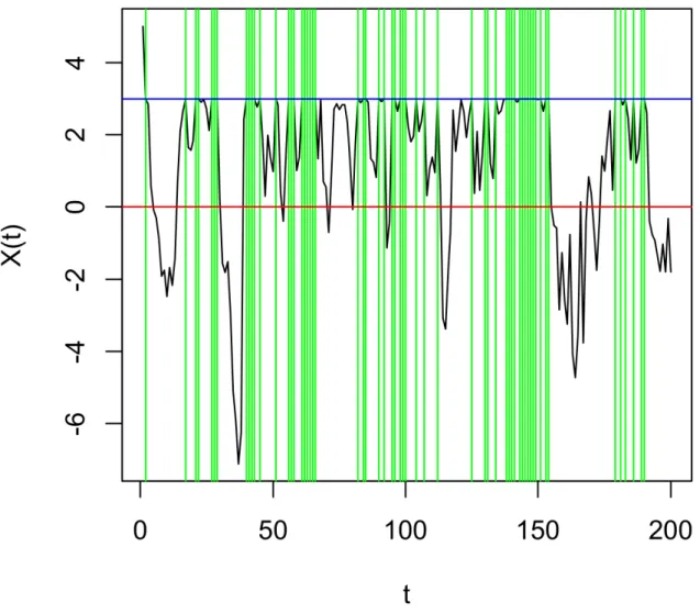
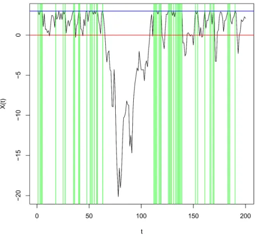
Figure 1.1: Regeneration block construction for AR(1) model.

As shown in [106] one can write the AR(p) process

Xn= ρ1Xn−1+ ρ2Xn−2+ · · · + ρkXn−k+ θn

in a Markovian form by constructing the multivariate sequence Yn = (Xn, · · · , Xn−k+1)�

and considering the process Y = {Yn, n ≥ 0}. Indeed, Y is a Markov chain whose ﬁrst

component has exactly the sample paths of the autoregressive process (see [106] for more details) and by Theorem 2.1 in [6] is a Harris recurrent Markov chain (see Example 2.6 in [6] for more details). Figure 2 illustrates the splitting technique for a trajectory of AR(1) process.

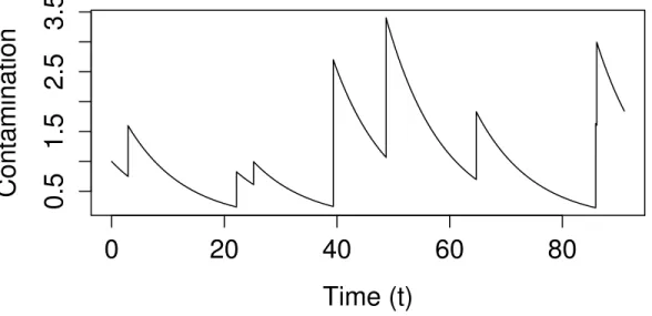
As the last example we present the Kinetic Exposure Model introduced in [31]. This process is an example of a piecewise deterministic Markov process (PDMP) (see also [25] for other examples how to relate the properties of the PDMPs (stationary distribution) with the properties of embedded chains possesing regenerative structure.

Example 3 (Kinetic Dietary Exposure Model). The Kinetic Dietary Exposure Model (KDEM) is a stochastic process that expresses the evolution of a contaminant in the human body along time. Let

(28)

0

20

40

60

80

0.5

1.5

2.5

3.5 Time (t)

Contamination

Figure 1.2: Kinetic Dietary Exposure Model which describes evolution of a contaminant in the human body.

• T1, · · · , Tn be the contaminant’s intake times

• ΔTn+1= Tn+1− Tn be the inter-intake time

• U1, · · · , Un be the contaminant’s intakes time at T1, · · · , Tn

The counting process {(N (t)}_t≥0 is deﬁned as

N (t) := #{i_{∈ N}∗ : Ti ≤ t}

for t≥ 0 is a renewal process and

A(t) = t_{− T}N (t)

is the backward recurrence time. We consider exposure process X(t) which dynamics is given by the ﬁrst order ordinary diﬀerential equation

dX(t) =−ωX(t)dt (1.3)

and ω > 0 is a ﬁxed parameter called elimination rate and corresponds to body’s metabolism dealing with the chemical elimination of contaminants. The total body burden of a given

(29)

dietary contaminant at time t is : X(t) = X(0) + N (t) � n=1 Un− N (t)+1 � n=1 � Tn∧t Tn−1 ωX(s)ds.

By solving (1.3), the exposure process is given by

X(t) = XTN(t)e

−ωA(t)

for any t_{≥ 0. The process {X(t)}}_t≥0(that is Xn= X(Tn)) is a PDMP. Let �X = (Xn)n∈N, be

an embedded chain of X. The evolution of the process �X is given by the following stochastic recurrence equation

Xn+1 = Xn× e−ω∆Tn+1+ Un+1, n ≥ 0

which is an autoregressive process with a random coeﬃcient.

Process �X plays an important role in the analysis of X, i.e. it describes the exposure process immediately after each intake (refer to [31] for details). Under some additional assumptions (speciﬁed for instance in [31]) it is possible to relate the continuous-time process X with the embedded chain �X. Figure 3 shows the trajectory of evolution of the contaminant in a human body along time.

3 A preview of contributions and future perspectives

As indicated in Section 1, this thesis focuses on developments in the ﬁeld of bootstrap and statistical learning when the data are Markovian. We start with uniform bootstrap central limit theorems for Harris recurrent Markov chains. Next, we generalize the wild and residual bootstrap procedures for autoregressive processes of order p to periodically autoregressive processes (PAR). PAR sequences can be written in a Markovian form and are an example of Harris recurrent Markov chains. The second part of the thesis focuses on applications of empirical processes theory to statistical learning. We derive exponential and polynomial type maximal inequalities in order to control the supremum distance between stationary distribution µ of the chain X and its empirical counterpart. Concentration inequalities of this type are crucial tool when proving the generalization bounds for statistical learning algorithms via empirical risk minimization approach (we encourage to look into [142], [144] and [38] for detailed treatment). In this thesis, we use this strategy in order to obtain generalization bounds for minimum volume set estimation problem.

Having given a very general outline of the thesis, we proceed with more detailed preview of contributions.

(30)

1. Uniform bootstrap central limit theorems for Harris recurrent Markov chains The ﬁrst contribution involves asymptotic results for Harris recurrent Markov chains and was published in [44], [45] and [25]. We extend the bootstrap central limit the-orem for the mean established in [26]. We show that uniform bootstrap CLT holds over uniformly bounded classes of functions F as well as in unbounded case when we only require second order moment conditions imposed on the envelope F of F. In this framework we measure the complexity of F by its covering number Np(�, Q, F) which

is interpreted as the minimal number of balls with radius � needed to cover F in the norm Lp(Q) and Q is a measure on E with ﬁnite support. In what follows, we impose

the ﬁniteness of the uniform entropy integral of F, namely � ∞

0

�

log N2(�, F)d� <∞, where N2(�, F) = sup Q

N2(�, Q, F).

More speciﬁcally, we show that under some technical conditions (speciﬁed in [44] and the second chapter of this thesis) imposed on X, f, class F and small set S and under the assumption _� ∞ 0 � log N2(�, F)d� <∞ we obtain that Z∗_n= n∗1/2_A_M   1 n∗ AM l∗ n−1 � i=1 f (B_i∗)− 1 �nAM �l�n−1 i=1 f ( �Bi)   (1.4)

converges in probability under Pν to a Gaussian process G indexed by F whose sample

paths are bounded and uniformly continuous with respect to the metric L2(µ). To

un-derstand Equation 1.4 we brieﬂy mention that n∗

AM and l

∗

n are bootstrap equivalents

of the quantities nAM and ln introduced in Subsection 2 and B∗i are bootstrap blocks

that is a sequence of i.i.d. blocks drawn with replacement from empirical distribu-tion funcdistribu-tion based on the regenerative blocks or the approximate ones (see page 19, Algorithm 2).

Our theorems are bootstrap versions of uniform central limit theorems for Harris chains for bounded classes of functions presented in [98] and in unbounded case (see [137]). Moreover, our proof techniques allow to apply our reasoning into regenerative case that enables simpliﬁcation of the proof of the uniform bootstrap central limit theorem for regenerative Markov chains established in [122]. Uniform central limit theorems (and their bootstrap versions) are an useful tool in non-parametric maximum likelihood estimation, kernel density estimation or wavelet density estimation (refer for instance to [110], [68] and [69] for details).

(31)

We are using the aforementioned results to establish bootstrap uniform central limit theorems for Fréchet differentiable functionals of Harris Markov chains. Under some technical conditions (uniform entropy condition, assumptions on a small set S, etc.) we have for a Fréchet differentiable functional at µ (with respect to a metric indexed by a class of functions, see [17] and Chapter 2 for details) that the bootstrap is asymp-totically valid. We have chosen to work with Fréchet differentiable functionals since it guarantees the existence of influence function useful when detecting the outliers in the data (see [140] for details).

2. Robust estimation for Markov chains with applications to PDMPs In our next contribution we propose a method to construct robust estimators for atomic regenerat-ive and Harris recurrent Markov chains with a special focus on Piecewise-Deterministic Markov Processes (PDMPs). In this framework we rely on a renewal theory for Markov chains and further developments of the approximate regenerative block bootstrap method. The main idea is to eliminate blocks having either too much contribution to the statistics of interest, or having a too large length.

It is known (see [29]) that some classical concepts of robust statistics can be naturally extended to a Markovian framework. For instance, one can deﬁne an inﬂuence function on the torus T =_∪∞

k=1Ek. Indeed, let PT denote the set of all probability measures on

the torus T and for any b_{∈ T, set}

L(b) = k if b_{∈ E}k, k _{≥ 1.}

Then the inﬂuence function on the torus can be deﬁned as follows.

Deﬁnition . (Inﬂuence function on the torus) Let (V,� · �) be a separable Banach space. Let T : PT → V be a functional on PT. If, for some L in PT,

t−1(T ((1_{− t)L + tδ}b)− T (L))

has a ﬁnite limit as t → 0 for any b ∈ T, the inﬂuence function T(1) _{: P}

T → V of the

functional T at L is then said to be well-deﬁned, and, by deﬁnition, one set for all b in T,

T(1)(b, L) = lim

t→0

T ((1_{− t)L + tδ}b)− T (L)

t . (1.5)

Now it is straightforward to define Fréchet differentiability of functionals of Markov chains.

(32)

Definition . (Fréchet differentiability of functionals of Markov chains) The functional T : PT → R is Fréchet differentiable at LA ∈ PT for a metric d, if there exists

a continuous linear operator DTLA (from the set of signed measures of the form L−LA

in (R,_{� · �)) and a function}

�(1)(·, LA) : R→ (R, � · �),

which is continuous at 0 and �(1)_{(0, L}

A) = 0 such that ∀ L ∈ PT, T (L)− T (LA) = DTLA(L− LA) + R (1)_{(L, L} A), where R(1)(L, LA) = d(LA, L)�(1)(d(LA, L), LA).

Furthermore, assume that T admits the following representation,

∀ LA∈ PT, DTLA(L− LA) =

�

T(1)(b, LA)L(db),

where T(1)_{(b, L}

A) is the inﬂuence function at LA.

Fréchet differentiability is a standard tool for obtaining central limit theorems for plug-in estimators. Indeed, suppose that T : PT → R is a Fréchet differentiable functional

at LA for some metric dF (see Chapter 3 for details) , where F is a permissible class

of functions with an envelope F, satisfying the uniform entropy condition � ∞ 0 � sup Q log N2(�, Q, F)d� <∞.

Assume in addition, in the regenerative atomic case

EA � � 1≤j≤τA F (Xj) �2 <∞, Eν(τA) < ∞, EA(τA2) < ∞. Then, n1/2(T (Ln)− T (LA))→ N � 0,V ar(T (1)_(B i, LA)) EA(τA) � .

We establish similar results for Harris recurrent Markov chains.

In this framework, we consider in particular the construction of robust estimators for the embedded Markov chains associated to the PDMP (which is a process whose

(33)

behaviour is determined by random jumps at points in time and its evolution is de-terministically ruled by an ordinary diﬀerential equation between those times).

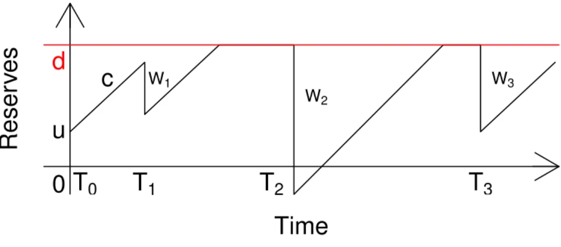
We consider robust estimators of several risk indicators such as the ruin probability, the expected shortfall and the extremal index of two PDMPs: the Cram´er-Lundberg with a dividend barrier and the Kinetic Dynamic Exposure Model (KDEM) used in modeling phamarcokinetics of contaminants (see [31] for instance).

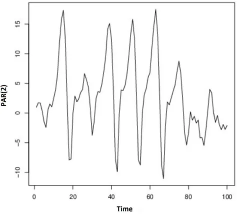
3. Wild and residual bootstrap methods for periodically autoregressive processes This contribution is published in [46]. We consider periodically autoregressive process (PAR) of the form

XnT +v = p � k=1 φk(v)XnT +v−k+ �nT +v, (1.6) where Φ� _{= [φ}₁_{(1), φ}₂_{(1), . . . , φ}_p_{(1), φ}₁_{(2), . . . , φ}_p_{(2), . . . , φ}₁_{(T ), . . . , φ}_p_{(T )]} designates the vector of parameters and�_{is a transpose. The {X}

nT +v} denotes the series

during the n-th cycle (0_{≤ n ≤ N − 1) during v-th season (1 ≤ v ≤ T ). The {�}nT +v}

is the mean zero white noise with variance of the form Var(�nT +v) = σv2 > 0 for all

seasons v. The process in (1.6) can be written in a Markovian form using analogous vectorization trick as in Example 2 since PAR process may be written as T -variate autoregressive model (AR), refer to [20] for details. We obtained the least squares estimators of model’s parameters

�

Φ� ₌�_φ�₁_{(1), �}_φ₂_{(1), . . . , �}_φ_p_{(1), �}_φ₁_{(2), . . . , �}_φ_p_{(2), . . . , �}_φ₁_{(T ), . . . , �}_φ_p_{(T )}� in order to generate their bootstrap equivalents.

We propose wild and residual bootstrap procedures which are data driven (since they do not require a choice of the length of bootstrap blocks), thus can be attractive for practical use. The residual bootstrap procedure for PAR processes consists of the following steps.

Residual bootstrap method for PAR processes Step 1 Compute the ordinary least squares estimator �Φ_{of Φ.} Step 2 Compute the residuals of the estimated model

��nT +v = XnT +v− p � k=1 � φk(v)XnT +v−k, where 1_{≤ v ≤ T, 0 ≤ n ≤ N − 1.}

(34)

Step 3 Compute the centred residuals ¯ ηnT +v = ��nT +v σv − 1 N T N −1_� n=0 T � v=1 ��nT +v σv ,

where N T is the number of all observations in the model. Step 4 Generate bootstrap variables η∗

nT +v by drawing randomly with replacement from

{¯η1, . . . , ¯ηN T}.

Step 5 Generate the bootstrap version of the model (1.6)

X_{nT +v}∗ = p � k=1 � φk(v)XnT +v−k+ σvη∗nT +v, 1≤ v ≤ T.

Step 6 Calculate the bootstrap estimators of parameters for each season v, 1 _{≤ v ≤ T} �

Φ∗_{(v), where}

z∗(v) =�X_v∗, . . . , X_{(N −1)T +v}∗ ��, 1_{≤ v ≤ T.}

The second method we propose is wild bootstrap procedure for PAR processes. Wild bootstrap method for PAR processes

Step 1 Compute the ordinary least squares estimator �Φ_{of Φ.} Step 2 Compute the residuals of the estimated model

��nT +v = XnT +v− p � k=1 � φk(v)XnT +v−k, where 1_{≤ v ≤ T, 0 ≤ n ≤ N − 1.}

Step 3 Generate the bootstrap process X_{nT +v}† for each season v, 1_{≤ v ≤ T} X_{nT +v}† = p � k=1 � φk(v)XnT +v−k+ �†nT +v and �†_{nT +v} _{= ��}nT +vηnT +v† ,

where η_{nT +v}† _{∼ N (0, 1) and (η}_{nT +v}† )_{nT +v∈R} _{is independent of ��}nT +v.

Step 4 Calculate the bootstrap estimator of parameters, namely �Φ†_{(v) for each season} v, 1_{≤ v ≤ T, where}

z†(v) = �Xv†, . . . , X_{(N −1)T +v}†

��

(35)

Next, we proved weak consistency for both methods. More specifically, we showed for a causal periodic autoregressive series XnT +vdefined in (1.6) with finite fourth moment

that, the residual bootstrap procedure we proposed is weakly consistent, i.e. √ N�Φ�∗_{− �}Φ�_{−→ N}P∗ �_{0, R}−1�_, where � Φ∗� ₌�_φ�∗ 1(1), �φ∗2(1), . . . , �φ∗p(1), �φ∗1(2), . . . , �φ∗p(2), . . . , �φ∗1(T ), . . . , �φ∗p(T ) �

is a vector of bootstrap estimators of parameters for each season v obtained from residual bootstrap algorithm and R is speciﬁed in Chapter 4. Similar consistency results are obtained for wild bootstrap procedure (see Chapter 4). Finally, we illustrate our theoretical considerations by simulations.

4. Exponential and polynomial type maximal inequalities for Harris Markov chains Motivated by applications in statistical learning we establish bounds for the tail probab-ility for suprema of empirical processes in a Markovian framework. These contributions are presented in [22], [23] and [24].

Let f : E _{→ R be a measurable function. Since our inequalities are maximal type,} we control the class of functions via uniform entropy number. Under exponential moments imposed on τAand f (Bj) we establish Bernstein and Hoeﬀding type maximal

inequalities as a function of uniform entropy number and moments of time returns and blocks. One of main diﬃculties when deriving such bounds is that even if we assume that f is bounded, f (Bj) may be unbounded over a whole block of observations. In

order to derive the inequalities we rely heavily on Montgomery-Smith’s inequality from [108] and symmetrization techniques from [119].

We also show that under weaker conditions imposed on time returns and f (Bj)�s,

the polynomial bounds can be established. Interestingly, the conditions imposed on a Markov chain X are satisﬁed by sub-geometrically ergodic Markov chains, to which our polynomial tail inequality can be applied.

Furthermore, we establish bounds for the expectation of the supremum of empirical process in a Markovian setting since they occur to be particularly useful when one wants to select a model via some penalization criterion with penalty term depending on a complexity of the whole collection of models.

We present the aforementioned results in a detailed form in the subsequent sections. However, to give a reader a general overview of obtained results we provide the bounds

(36)

in a general (and somewhat simpliﬁed) form below. The detailed conditions imposed on chain X are omitted here and stated in further sections. For the sake of simplicity we provide the results solely in the atomic regenerative case (we formulate the inequalities for Harris recurrent Markov chains in further sections). Let

σ_m2 = max

f ∈F σ

2_{(f ) > η > 0.}

• Bernstein type maximal inequality Assume that N1(�, F) <∞. Then, under

exponential block moment conditions and exponential moments of return times to set A, we have for any x > 0, 0 < � < x/2 and for all n_{≥ 1}

Pν � sup f ∈F � � � � � 1 n n � i=1 f (Xi)− µ(f) � � � � �≥ x � ≤ N1(�, F) K1 � exp � −n(x − 2�)2 K2(σ2m+ K3(x− 2�)) �� ,

where K1, K2 and K3 are positive parameters speciﬁed in Chapter 5.

• Hoeﬀding type maximal inequality Assume that N1(�, F) <∞. Suppose

fur-ther that the class of functions F is uniformly bounded. Then, under exponential block moment conditions and exponential moments of return times to set A, we have for any x > 0, 0 < � < x/2 and for all n_{≥ 1}

Pν � sup f ∈F � � � � � 1 n n � i=1 f (Xi)− µ(f) � � � � �≥ x � ≤ N1(�, F) L1 � exp � −n(x− 2�) 2 L2D2 �� ,

where D is a constant such that _{∀f ∈ F |f| < D and L}1 and L2 are positive

parameters speciﬁed later in Chapter 5.

• Polynomial tail maximal inequality Assume that N1(�, F) < ∞. Suppose

further that the p−th block moment and p-th moment of return times to the atom A are ﬁnite. Then, we have for any x > 0, 0 < � < x/2 and for all n≥ 1

Pν � sup f ∈F � � � � � 1 n n � i=1 f (Xi)− µ(f) � � � � �≥ x � ≤ C1 N1(�, F) (x_{− 2�)}p_np/2

and C1 is a positive parameter speciﬁed in Chapter 5.

• Bound for expectation of supremum of empirical processes Assume that

(37)

where F is an envelope for F. Moreover, suppose that uniform entropy number N1 � � R1, F �

<_{∞. Then, for any � > 0 we have} E_A � sup f ∈F � � � � � 1 n ln � i=1 (f (Bi)− µ(f(B1))) � � � � � � ≤ R2    �+ N � � R1 , F � × EA[F (B1)2]1/2 � � � �2logN1 � � R1, F � n     , where R1 and R2 are positive constants that can be explicitly computed.

The above results may be easily generalized to a Harris recurrent case.

5. Generalization bounds for minimum volume set estimation problem The last contributions presented in this thesis are generalization bounds for minimum volume set (MV-set) for regenerative and Harris recurrent Markov chains. The results have been presented in [23] and [24]. The MV-set estimation problem was ﬁrstly proposed in [120] in the i.i.d. setting.

Let µ be a probability distribution on a measurable space (E, E). Let α_{∈ (0, 1) and λ} be a σ-ﬁnite measure of reference on (E, E), any solution of the minimization problem (1.7)

min

Ω∈E λ(Ω) subject to µ(Ω)≥ α (1.7)

is called a M V -set of level α. The distribution µ is assumed to be absolutely continuous w.r.t. λ and denote by

f (x) = (dµ/dλ)(x) the related density.

Under some technical assumptions on f , for any α∈ (0, 1), [120] showed that the set Ω∗

α = {x∈ E : f(x) > γα},

where γα is the unique number such that

�

f (x)>γα

f (x)dλ(x) = α

is the unique solution of the MV-set estimation problem (1.7). Minimum volume sets can be interpreted as follows, for small values of the mass level α, M V -sets enable to

(38)

recover the modes of the distribution, while their complementary sets correspond to

rare observations when α is large.

In practice, distribution µ is unknown and is replaced by its empirical counterpart µn. Then ﬁnding ﬁnding a minimum volume set of level α boils down to solving the

following minimization problem min

Ω∈E λ(Ω) subject to �µn(Ω)≥ α − ψn (1.8)

with ψn being a tolerance parameter (see Chapter 6 for more details).

The minimum volume set estimation technique can be used as an unsupervised anomaly detection algorithm since when dealing with unlabelled data we consider anomaly as a rare event.

Scott and Nowak [126] established generalization bounds for MV-set estimation prob-lem in the i.i.d. setting. In order to establish generalization bounds in a Markovian setting we retract to the framework of empirical risk minimization and thus, heavily rely on concentration inequalities which allows us to control the suprema of empirical processes involved. Our approach boils down to decomposition of empirical distribution function of interest into: ∀ Ω ∈ E,

� µn(Ω) = 1 n τA � i=1 I{Xi ∈ Ω}+ ln− 1 n � 1 ln− 1 l�n−1 j=1 Sj(Ω) � +1 n n � i=1+τA(ln) I{Xi ∈ Ω}, (1.9)

where ln = �n_i=1I{Xi ∈ A} denotes the number of visits to set A (regenerations),

the occupation time of the set Ω between the j-th and (j + 1)-th regeneration times is denoted by Sj(Ω) = �τA(j)<i≤τA(j+1)I{Xi ∈ Ω}. Decomposition (1.9) along with

application of polynomial tail maximal inequality for Markov chains allows us to extend the result in [126] to the atomic regenerative and Harris recurrent case.

Let p_{≥ 2. In order to establish generalization bounds for minimum volume set} estim-ation problem we assume that

E_A[τ_Ap] <_{∞ and E}ν[τ_Ap] <∞.

Let r _{≥ 1. The collection of indicator functions on E,} F = {I{x ∈ Ω} : Ω ∈ G}

is a uniform Donsker class (relative to L1) with polynomial uniform covering numbers,

i.e. there exists a constant c > 0 s.t. _{∀ζ > 0,}

N1(ζ, F) def

= sup

Q

Bootstrap and uniform bounds for Harris Markov chains

HAL Id: tel-01988595

https://pastel.archives-ouvertes.fr/tel-01988595

Bootstrap and uniform bounds for Harris Markov chains

Gabriela Ciolek

To cite this version:

TH`

ESE DE DOCTORAT

l’Universit´

e Paris-Saclay

Math´ematiques appliqu´ees

Gabriela CIO�LEK

Bootstrap and uniform bounds for Harris Markov chains

Acknowledgements

List of publications

Published articles, chapters and conference papers

Articles in revision

Contents

Chapter 1

Introduction

1

Motivation

2

Basic properties of regenerative and Harris recurrent

Markov chains

2.1

Regenerative Markov chains

2.2

General Harris Markov chains and the splitting technique

2.3

Regenerative blocks for dominated families

2.4

A few examples of regenerative and Harris recurrent Markov

chains

0

20

40

60

80

0.5

1.5

2.5

3.5

Time (t)

Contamination

3

A preview of contributions and future perspectives