Partial Move A*
Tristan Cazenave
LAMSADE Universit´e Paris-Dauphine
Paris, France
Abstract—Some shortest path problems that can be solved using the A* algorithm have a large branching factor due to the combination of multiple choices at each move. Multiple sequence alignment and multi-agent pathfinding are examples of such problems. If the search can be stopped after each choice instead of being stopped at each combination of choices, it takes much less memory and much less time. The goal of the paper is to show that Partial Move A* is much better than A* for these problems when the branching factor is large due to a large combination of choices at each move. When there is such a large combination of choices at each move, Partial Move A* can yield large memory gains and speedups over regular A*.
I. INTRODUCTION
When the moves of a problem contain multiple choices, the evaluation of each choice separately can be interesting instead of evaluating all the possible combinations of choices. When each choice is evaluated separately the search can be stopped at a partial move instead of being stopped at each combination that contains this partial move. Partial Move A* (PMA*) is an iterative deepening A* algorithm [1] that stops search inside a move. It can yield large memory gains and speedups on difficult problems. The algorithm can be applied to multiple sequence alignment and to multi-agent pathfinding. We show in this paper that it enables large memory gains and large speedup on these two problems when the branching factor is large.
Multiple sequence alignment is an NP-hard problem that can be addressed with the A* algorithm [2]. It is commonly believed that iterative deepening A* is not appropriate for mul-tiple sequence alignment since there are many paths passing through the same nodes, with the exception of the work on iterative deepening dynamic programming [3]. We show that PMA* is appropriate for multiple sequence alignment even if it is an iterative deepening A* algorithm.
The multi-agent pathfinding problem is PSPACE-hard [4]. Existing literature on the multi-agent pathfinding problem mainly deals with inexact algorithm as the problem is con-sidered intractable. An example of an algorithm combining individual paths is cooperative pathfinding [5]. We are inter-ested in exact algorithms for this problem. The standard exact algorithm is A*. PMA* improves much on A* search for this problem. PMA* is complete and optimal for the multi-agent pathfinding problem. There are good approximation algorithms for this problem such as [6], however these algorithm are not complete nor optimal.
An algorithm related to PMA* is Partial Expansion A* [7]. Partial Expansion A* uses less memory than A* but uses more
time, whereas PMA* uses less memory than A* and less time on difficult problems. PMA* also uses less memory and less time than Partial Expansion A*.
The idea underlying PMA* is that it is very beneficial both for memory consumption and for speed to be able stop search at each move component. For example in multiple sequence alignment it is important to be able to stop search after each choice of either aligning a letter in a sequence or inserting a gap in the same sequence. Concerning multi-agent pathfinding it is important to be able to stop search after the move of each agent and not only after all the agents have moved.
The outline of this paper is as follows: section 2 compares A*, Partial Expansion A* and Partial Move A*. Section 3 presents the application of PMA* to multiple sequence alignment and section 4 presents its application to multi-agent pathfinding.
II. COMPARISON OF ALGORITHMS FORA*
In this section the differences between A*, Partial Expan-sion A* and PMA* are outlined.
A. A*
In A*, all the children of a node are added to the Open structure, and the node is placed in the closed structure after expansion.
B. Partial Expansion A*
Partial expansion A* does not expand all the children of a node. It selects the children that have a F value smaller than the F value of the node plus a constant C.
It defines two sets :
𝑆𝑈𝐶𝐶≤𝐶 ← {𝑛𝑗∣𝑛𝑗∈ 𝑠𝑢𝑐𝑐(𝑛), 𝑓(𝑛𝑗) ≤ 𝐹 (𝑛) + 𝐶} 𝑆𝑈𝐶𝐶>𝐶 ← {𝑛𝑘∣𝑛𝑘∈ 𝑠𝑢𝑐𝑐(𝑛), 𝑓(𝑛𝑘) > 𝐹 (𝑛) + 𝐶} It only expands the children in𝑆𝑈𝐶𝐶≤𝐶and puts the node n in the closed nodes only if 𝑆𝑈𝐶𝐶>𝐶 = ∅.
Each time the algorithm comes again on an already partially expanded node, it has to develop again the node in order to build the SUCC sets of nodes. When there are many sequences, the computing time of the algorithm is dominated by the computation of the SUCC sets.
C. Partial Move A*
When running Partial Expansion A* on problems with a large number of children for each node, most of the time of the algorithm is consumed in finding all the possible children of a node and computing the sets𝑆𝑈𝐶𝐶≤𝐶 and𝑆𝑈𝐶𝐶>𝐶. For
example when aligning nineteen protein sequences the number of children of a node is219− 1 and almost all the computing time of the algorithm is taken in finding the relevant children in𝑆𝑈𝐶𝐶≤𝐶. Partial Move A* uses iterative deepening to find all the children, therefore it stops its search well before the expansion of all the children and uses much less time.
Moreover, due to the C constant, Partial Expansion A* will maintain nodes in the Open structure that have a F greater than the minimal F of the Open structure. In contrast Partial Move A* will never have nodes in its structures that have a F greater than the F under consideration. Therefore Partial Move A* uses less memory than Partial Expansion A*.
Algorithm 1 Pseudo-code for Partial Move A*.
PMA (int g, int index, position previous, position current) f = g + h (index, previous, current)
if f > f of current iteration then
return false;
end if
if index = number of steps in a move then if h (current) = 0 then
return true;
end if
if currentPosition already visited with a smaller g then
return false;
end if
add current to already visited index ← 0
previous ← current
end if
for all possible partial moves do
compute 𝛿𝑔 the increase in g due to the partial move update current with the partial move
if PMA(g +𝛿𝑔, index + 1, previous, current) then
return true;
end if end for
return false
Partial nodes are the states of the search that corresponds to incomplete moves, nodes are the states that correspond to complete moves. In multi-agent pathfinding for example a partial move is moving one agent to one of its neighbor locations whereas a complete move is moving all the agents to one of their neighbor locations. In multiple sequence alignment a partial move consists in choosing to insert a gap or not in the current location of a DNA string, whereas a complete move consists in choosing to inster a gap or not for all the DNA strings.
At the beginning of algorithm 1 the value of 𝑓 for the current partial node is computed. If this value is greater than the f of the current iteration the algorithm is stopped since the path has a greater cost than the bound on f.
If the state corresponds to a node (i.e. the move is complete and𝑖𝑛𝑑𝑒𝑥 = number of steps of a move), then it returns true if the goal is achieved , else it stops search if a transposition
10+6 11+5 12+4 13+3 15+3 14+4 17+3 13+5 14+4 16+4 15+3 17+3 17+3 19+3 15+3
Fig. 1. The expansion behavior of A*.
occurs, or it update the hash table and starts a new move. Then comes the recursive call for all possible choices of a partial move. The recursive call has an updated position in the state space and an updated𝑔 as parameters.
As Partial Move A* is an iterative deepening algorithm, algorithm 1 is iteratively called with algorithm 2.
Algorithm 2 Pseudo-code for iterative deepening Partial Move
A*.
iterativePMA ()
f of current iteration = h (root)
while true do
init hash table
add root to already visited
if PMA (0, 0, root, root) then
return f of current iteration;
end if
f of current iteration = f of current iteration + 1
end while
D. Comparison on a simple example
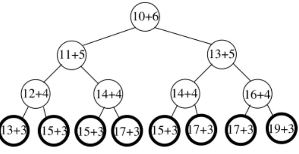
Suppose that a move is composed of three steps and that at each step there is a choice between two partial moves: a move on the left that costs 1 and a move on the right that costs 3. The admissible heuristic is the number of partial move before the goal.
A* will create the 23 = 8 children, insert them in the Open structure and remove the developed node from the Open structure. The tree developed by A* and the created nodes are given in figure 1. Each partial node contains its g value plus its h value. All the leaves are in bold meaning they are inserted in the Open structure. The root of the tree of figure 1 is a complete node as well as the leaves, the other nodes are partial nodes.
Partial Expansion A* will create the 23 = 8 children, if the constant 𝐶 = 2 it will only keep the children that have a 𝐹 ≤ 18 and insert them in the Open structure. The tree developed by Partial Expansion A* is given in figure 2 and the new open nodes are in bold.
Partial Move A* with the threshold for f of current iteration = 17 will only develop one node as in figure 3. We see in this example that Partial Move A* develops less nodes than A* and Partial Expansion A* and uses less memory.
10+6 11+5 12+4 13+3 15+3 14+4 17+3 13+5 14+4 16+4 15+3 17+3 17+3 19+3 15+3
Fig. 2. The expansion behavior of Partial Expansion A*.
10+6 11+5 12+4 13+3 15+3 14+4 13+5
Fig. 3. The expansion behavior of Partial Move A*.
III. MULTIPLESEQUENCEALIGNMENT
The first subsection presents the multiple sequence align-ment problem and the related algorithms, the second sub-section details the PMA* algorithm for multiple sequence alignment, the third subsection gives experimental results comparing A* and PMA* on the alignment of real sequences.
A. The problem
Multiple sequence alignment is one of the most important problem in computational biology. The multiple sequence alignment problem can be considered as a shortest path problem in a s-dimensional lattice [8]. When aligning two sequences, we can construct a matrix and write the letters of the first sequence on the horizontal axis above the matrix, and the letters of the second sequence on the vertical axis at the left of the matrix. Each possible alignment starts at the upper left element of the matrix. For each element of the matrix there are three possible moves: the diagonal, the horizontal, and the vertical moves. A diagonal move is equivalent to aligning two characters of the sequences, an horizontal move is equivalent to aligning a character of the horizontal sequence with a gap in the second sequence, a vertical move aligns a character of the vertical sequence with a gap in the horizontal sequence. All alignments stop at the bottom right of the matrix after the last two characters of both sequences have been aligned.
The simple model to evaluate the cost of a move is: 0 for a match (aligning the two same characters), 1 for a mismatch, and 2 for a gap (a gap is represented with a -). The cost of a path is the sum of the costs of its moves.
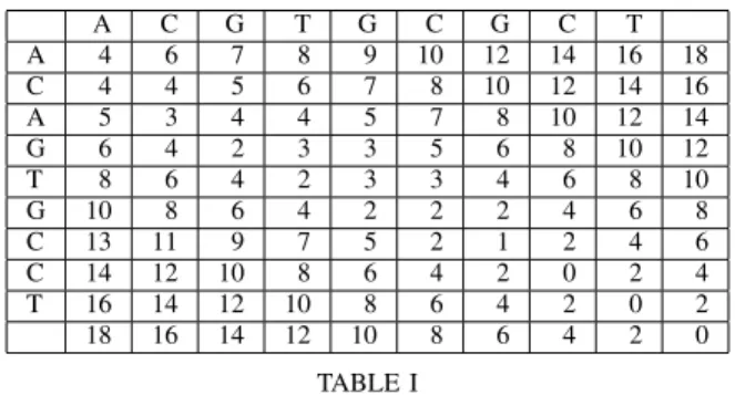
For example, if the first sequence is ACGTGCGCT and the second sequence is ACAGTGCCT the best alignment is:
A C G T G C G C T A 4 6 7 8 9 10 12 14 16 18 C 4 4 5 6 7 8 10 12 14 16 A 5 3 4 4 5 7 8 10 12 14 G 6 4 2 3 3 5 6 8 10 12 T 8 6 4 2 3 3 4 6 8 10 G 10 8 6 4 2 2 2 4 6 8 C 13 11 9 7 5 2 1 2 4 6 C 14 12 10 8 6 4 2 0 2 4 T 16 14 12 10 8 6 4 2 0 2 18 16 14 12 10 8 6 4 2 0 TABLE I
EXAMPLE OF A DYNAMIC PROGRAMMING TABLE.
AC-GTGCGCT ACAGTGC-CT and it has a cost of four.
When aligning s sequences, the path goes through a s-dimensional lattice, the branching factor is 2𝑠− 1, and the cost of a move is the sum of the costs of the moves for each pair of sequences.
Much more elaborate models of the cost of a mismatch such as the PAM matrices [9] have been developed and have been widely used. In order to keep things simple and as our interest is the search behavior of the alignment algorithms, we have restricted ourselves to the simple model.
Dynamic programming can be used to find exact alignments. However if the average length of the sequences to align is
𝑙𝑒𝑛𝑔𝑡ℎ, and the number of sequences is 𝑠, dynamic
program-ming needs O(𝑙𝑒𝑛𝑔𝑡ℎ𝑠) memory and time.
Table I gives the dynamic programming table corresponding to the previous two sequences. For each pair of index in the two sequences, the table gives the cost of the optimal alignment starting at the corresponding position. Each entry is computed as the minimum among the entry to the left plus 2, the entry below plus 2 and the entry to the lower left diagonal plus the cost of aligning the two corresponding letters. The table is computed starting at the lower right and going from the right to the left and then bottom-up. The upper left cell contains four which is the cost of the optimal alignment.
A* can be used for the optimal alignment of multiple sequences [2]. The admissible heuristic is computed using the dynamic programming tables for the pairwise alignments. Despite being more memory efficient than dynamic program-ming, A* is still limited by memory. In order to reduce the memory requirements, A* with partial expansion was proposed [7]. It consists in not memorizing in the open list, child nodes that have a𝑓 value greater than the addition of the
𝑓 value of their parent and of a threshold. Experimental results
show that Partial Expansion A* can align seven sequences using fewer stored nodes than A* (approximately 20 times less nodes), and can align some eight sequences problems that A* cannot align. However the gain in memory is acquired at the cost of a greater search time.
The admissible heuristic (the ℎ value) we have used for A* is the sum of the pairwise alignments given by the
2-dimensional dynamic programming tables.
B. The algorithm
As many paths go through the same nodes, it is important to detect a node that has the same position as another previous node and that has a greater or equal g. In that case the node has to be cut. It would be time consuming to go through all previous nodes, so we use a hash table with 65,535 entries in order to speedup the recognition of already developed nodes. The same hash table is used for A* and PMA*.
The four parameters of PMA* are:
∙ 𝑔 an integer containing the cost of the path up to the current position,
∙ 𝑖𝑛𝑑𝑒𝑥 an integer representing the sequence where the move is (there are two possible choices: inserting a gap or going forward in the sequence),
∙ 𝑝𝑟𝑒𝑣𝑖𝑜𝑢𝑠 a structure representing the previous position in the state space. The structure contains an array of integers, each integer contains the position in the cor-responding sequence,
∙ 𝑐𝑢𝑟𝑟𝑒𝑛𝑡 a structure representing the current position of the algorithm in the state space.
PMA* starts with the computation of the admissible heuris-tic. If the choice of the move is already made in the two sequences to evaluate, or if the move is not chosen in any of the two sequences then the contribution of the two sequences to the admissible heuristic is the usual score of the dynamic programming table, as in usual A*. However if the move is known in one sequence and not in the other, the contribution to the admissible heuristic is the minimum of the score if the move to play is a gap and of the score if the move to play is a forward move.
Once the admissible heuristic is computed, the 𝑓 value can be computed, and if it is greater than the current threshold f
of current iteration the node can be cut.
Otherwise, PMA* tests if all the sequences have been moved (in this case 𝑖𝑛𝑑𝑒𝑥 equals 𝑛𝑏𝑆𝑒𝑞𝑢𝑒𝑛𝑐𝑒𝑠). If ℎ equals 0 then the alignment is completed and the search stops. If the state has already been visited with a smaller or equal 𝑔, it can be detected by looking up in the hash table, in this case the node is cut. Otherwise the state is added to the hash table, the new partial move starts with the first sequence (𝑖𝑛𝑑𝑒𝑥 is set to 0), and the previous state is set to the current state.
Then comes the choice of the move in sequence𝑖𝑛𝑑𝑒𝑥. If a gap is chosen, then g is augmented of 2 for each previous sequence that has moved forward. If a move forward is chosen, then g is augmented of 2 for each previous sequence that has chosen a gap, and augmented of 1 for each sequence that has moved forward with a different letter. In each case, a recursive call with the updated g and the next sequence is performed.
Special care has to be taken for the admissible heuristic of PMA* since the usual admissible heuristic for multiple sequence alignment has to be extended to partial nodes. The usual heuristic for A* is the sum of the pairwise alignments computed with two dimensional dynamic programming tables. When extending it to partial nodes, we must take into account
that a partial move has been made in the sequences before
𝑖𝑛𝑑𝑒𝑥 and not in the sequences after 𝑖𝑛𝑑𝑒𝑥. In this case, in
order to be admissible, the heuristic must retain the less favor-able scenario between the insertion of a gap in the sequence after the 𝑖𝑛𝑑𝑒𝑥 and a move forward in the same sequence. The extended admissible heuristic is given in algorithm 3.
Algorithm 3 Pseudo-code for computing the admissible
heuristic at a partial move.
h (int index, position previous, position current) h = 0
for i from 0 to nbSequences - 1 do for j from i + 1 to nbSequences - 1 do
if ((i< index) and (j ≥ index)) then
increase h by the minimum cost between inserting a gap in sequence j and moving forward in sequence j plus the pairwise heuristic
else
increase h by the pairwise heuristic
end if end for end for
return h
C. Example of a search
In order to explain how PMA* behaves for multiple se-quence alignment we compare it to A* for the alignment of the three following DNA strings:
ACGTGCGCT ACAGTGCCT ATGCAACCT
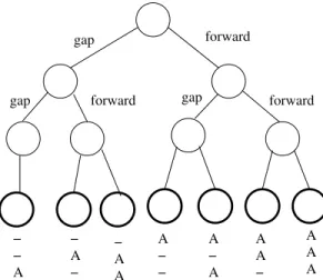
The behavior of A* for the aligning the first three letters is given in figure 4. A* inserts all possible alignments of the three letters in the open list. The behavior of PMA* for aligning the same three letters with a f limited to 0 is given in figure 5. Here we can see that PMA* is much more selective about the nodes to develop. The behavior of PMA* for a threshold of 2 is given in figure 6. We see here that four moves out of six are played (the bold circles). However these examples only involve three DNA strings. When aligning 20 DNA strings (this example cannot easily be given in a figure), a PMA* with a threshold of 2 will only play one move whereas A* and Partial Expansion A* will try220 different moves. Playing as many moves is much more slower and is much more memory consuming.
D. Results for real sequences
PMA* and A* were compared on real sequences from Balibase [10]. The memory limit for both algorithms was set to 10,000,000 nodes. Both algorithms use a hashtable of 65,535 entries. The open nodes of A* are stored in an array of stacks and therefore finding the best open node takes a very small constant time. All nodes are pre-allocated, therefore no time is spent in memory allocation.
forward gap
gap forward gap forward
− − A − A − − A A A − − A − A A A − A A A Fig. 4. Behavior of A* for the first move of the sequence.
forward
forward
A A A
Fig. 5. Behavior of PMA* for a𝑓 threshlod of 0.
forward gap
forward gap forward
− A A A − A A A − A A A
Fig. 6. Behavior of PMA* for a𝑓 threshold of 2.
𝑛𝑎𝑚𝑒 𝑠 𝑎𝑙𝑔𝑜. 𝑡𝑖𝑚𝑒 𝑛𝑜𝑑𝑒𝑠 2trx-ref2 20 PMA* 19,043.88 2,021,479 2trx-ref2 19 PMA* 500.66 95,732 2trx-ref2 18 PMA* 9.95 3,718 2trx-ref2 17 PMA* 1.18 769 2trx-ref2 16 PMA* 0.44 452 2trx-ref2 16 A* 138.03 9,244,517 1tvxA-ref2 15 PMA* 15.08 15,779 1tvxA-ref2 15 A* >242.42 >10,000,000 1tvxA-ref2 14 PMA* 0.99 1,587 1tvxA-ref2 14 A* 147.73 7,490,488 1tvxA-ref2 13 PMA* 0.44 908 1tvxA-ref2 13 A* 13.28 2,127,596 1tvxA-ref2 12 PMA* 0.09 309 1tvxA-ref2 12 A* 0.93 509,547 1tvxA-ref2 11 PMA* 0.03 178 1tvxA-ref2 11 A* 0.22 202,299 1aboA-ref1 5 PMA* 8.21 414,817 1aboA-ref1 5 A* 2.23 475,654 TABLE II
RESULTS FOR SEQUENCES FROMBALIBASE.
𝑛𝑎𝑚𝑒 𝑠 𝑠𝑝𝑒𝑒𝑑𝑢𝑝 𝑔𝑎𝑖𝑛 2trx-ref2 16 313.70 20,452.47 1tvxA-ref2 14 149.22 4,719.90 1tvxA-ref2 13 30.18 2,343.17 1tvxA-ref2 12 10.33 1,649.02 1tvxA-ref2 11 7.33 1,136.51 1aboA-ref1 5 0.27 1.15 TABLE III
SPEEDUP AND GAIN FOR SEQUENCES FROMBALIBASE.
Table II gives the time and nodes used by PMA* and A* on some real sequences. The first line of the table shows that PMA* is able to align optimally the first 20 sequences of 2trx-ref2. On the same set of sequences, A* can only align the first 16 sequences in 9,244,517 nodes and 138.03 seconds as can be seen from line 6 of the table, whereas PMA* can align the same 16 sequences in 452 nodes and 0.44 seconds. A* cannot align the first 15 sequences of 1tvxA-ref2 when PMA* can align them in 15,779 nodes. The last result shows that for a small number of sequences (in this case the 5 sequences of 1aboA-ref1), PMA* still uses a little less memory than A* but takes more time.
Table III gives the speedup and memory gain of PMA* over A*. They increase with the number of sequences to align.
IV. MULTI-AGENT PATHFINDING
The first subsection presents the multi-agent pathfinding problem, the second subsection details the application of PMA* to the problem, the third subsection experimentally compares A* and PMA* for the exchanging places problem, the fourth subsection compares them for the random locations problem.
A. The problem
The multi-agent pathfinding problem consists in finding a minimal path for multiple agents that move on the same
map. Agents cannot occupy the same location so they have to cooperate to find a path that is globally minimal.
A* can be used to find an optimal path. The natural admissible heuristic is to sum the Manhattan distances of the agents to their goal locations. At each step of the algorithm, each agent has five choices (left, right, up, down and stay idle), therefore the branching factor is5𝑛𝑏𝐴𝑔𝑒𝑛𝑡𝑠.
When an agent decides not to move, the contribution of the agent to the global cost is 0 if the agent is on its goal location, otherwise it is 1. It means the𝑔 value contains the number of times the agents were not on their goal locations.
In multi-agent pathfinding, the same admissible heuristic is used both for A* and PMA*. It consists in the sum of the Manhattan distances to the goal locations.
B. The algorithm
As for multiple sequence alignment, we use a hash table with 65,535 entries in order to speedup the recognition of already developed nodes. The same hash table is used for A* and PMA*. A* nodes are also pre-allocated and no time is used in memory allocation, the best open node is retrieved in a small constant time by A* using an array of stacks.
As in multiple sequence alignment, PMA* takes four pa-rameters, the 𝑔 value, the agent to move, the previous state and the current state. The admissible heuristic of PMA* for multi-agent pathfinding is the same as the admissible heuristic of A*. It consists in computing the sum of the Manhattan distances of all the agents to their goal locations. If ℎ equals 0 the problem is solved, if𝑓 is greater than the f of the current
iteration threshold the node is cut.
If all agents have chosen their moves (in this case 𝑖𝑛𝑑𝑒𝑥 equals 𝑛𝑏𝐴𝑔𝑒𝑛𝑡𝑠), the node is inserted in the hash table if it is not already present with a smaller or equal 𝑔, and another move starts with 𝑖𝑛𝑑𝑒𝑥 set to 0 and the previous state set to the current state.
Then comes the choice of the move for the𝑖𝑛𝑑𝑒𝑥 agent, for each neighbor if the move to the neighbor is possible (it is not occupied, there is no other agent on it at next turn and there is no swap between two agents), the recursive call is performed with𝑔 and 𝑖𝑛𝑑𝑒𝑥 increased by one.
The other possibility for an agent is to stay at the same location, it is possible only if another agent has not chosen to move to this location. If the location is the goal location, the cost of staying on it is 0, otherwise it is 1. The recursive call is performed with an updated 𝑔 and the next agent (𝑖𝑛𝑑𝑒𝑥 + 1).
C. The exchanging places problem
The problem of exchanging places involves an even number of agents. Each agent faces another agent on an empty map and they have to exchange places. Partial Move A* solves the problem of exchanging places depicted in table IV in 2.46 seconds and 79,631 nodes, whereas A* does not solve the problem in 8,599 seconds and 40,000,000 nodes. Table V compares A* and Partial Move A* on instances of the problem going from 2 agents to 8 agents. The gain and the speedup
𝑎1 𝑎2 𝑎3 𝑎4
𝑎5 𝑎6 𝑎7 𝑎8
TABLE IV
EXCHANGING PLACES FOR8AGENTS.
Agents A* nodes PMA* nodes gain
2 216 11 19.64
4 30,713 181 169.69
6 5,233,301 3,671 1425.58
8 >40,000,000 79,631 >502.32 A* time PMA* time speedup 2 0.003281 s. 0.000793 s. 4.14 4 0.011146 s. 0.001565 s. 7.12 6 236.91 s. 0.038093 s. 6,219.25 8 >8,599 s. 2.46 s. >3,495.53
TABLE V
OPTIMAL EXCHANGING PLACES FOR DIFFERENT NUMBERS OF AGENTS.
increase with the number of agents, we could not complete the A* search for 8 agents since it exhausted memory.
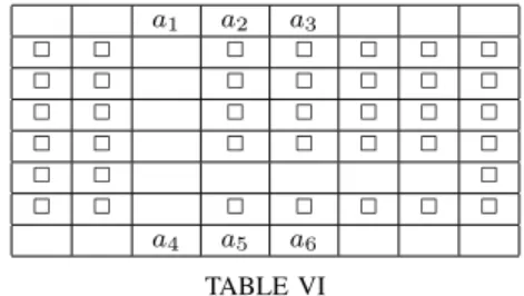
Since exchanging places on an empty map can be solved by cooperative pathfinding algorithms, we also tested PMA* and A* on problems that are more difficult to solve by algorithms that combine individual paths. Table VI gives an example of the problem of exchanging places in a corridor for 6 agents,
𝑎1has to go where𝑎6is and𝑎6has to go where𝑎3is,𝑎2 has to exchange place with𝑎5 and𝑎3 has to go to𝑎4whereas𝑎4 has to go to𝑎1.
Table VII compares A* and PMA* on the problem of exchanging places in a corridor for up to 7 agents. As in this problem the branching factor is small due to the configuration of the map, the speedups and gains are smaller than in problems with a larger branching factor.
D. The random locations problem
In order to see the evolution of the gains and speedups of Partial Move A* over A*, an experiment involving random problems was conducted. All the problems involve an 8 × 8 empty map. The initial locations of the agents as well as their
𝑎1 𝑎2 𝑎3 □ □ □ □ □ □ □ □ □ □ □ □ □ □ □ □ □ □ □ □ □ □ □ □ □ □ □ □ □ □ □ □ □ □ □ □ □ □ 𝑎4 𝑎5 𝑎6 TABLE VI
Agents A* nodes PMA* nodes gain 2 142 43 3.30 3 732 131 5.59 4 14,615 4,648 3.14 5 99,930 19,026 5.25 6 1,968,778 436,038 4.52 7 12,746,247 1,752,622 7.27
A* time PMA* time speedup 2 0.002742 s. 0.001031 s. 2.66 3 0.002863 s. 0.001433 s. 1.87 4 0.019157 s. 0.041990 s. 0.46 5 0.242978 s. 0.296548 s. 0.82 6 108.260582 s. 29.794621 s. 3.63 7 10,122.378906 s. 268.604767 s. 37.69 TABLE VII
OPTIMAL EXCHANGING PLACES IN A CORRIDOR FOR DIFFERENT NUMBERS OF AGENTS.
Agents mean gain median gain max gain
2 18.53 19.29 46.00 3 86.39 94.50 193.00 4 364.93 415.62 1,248.50 5 1,586.63 1,827.88 8,339.25 6 3,325.39 7,608.50 89,977.16 7 14,438.44 23,743.57 602,400.31 8 >26,698.17 122,229.20 4,125,671.00 TABLE VIII
MEMORY GAINS FOR UP TO8AGENTS.
goal locations are chosen at random on the map. Problems for 1 to 8 agents were randomly generated. For each possible number of agents, Partial Move A* and A* were compared on 100 problems. Table VIII gives the mean, median and maximum memory gains over the 100 problems for each number of agents. Table IX gives similar information for the speedups. Multiple problems involving 8 agents could not be solved by A* within the 40,000,000 nodes limit. Therefore the mean values for 8 agents are lower bounds.
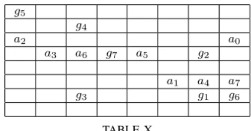
Table X gives the problem that has the maximal speedup of 4,049,291.25 and the maximal memory gain of 2,222,222.25. The agents are noted𝑎0to𝑎7and their respective goal location
𝑔0 to 𝑔7, 𝑔0 is under 𝑎6. This problem is solved in 9 nodes and 0.000264 seconds by Partial Move A*, whereas A* solves it in 37,131,039 nodes and 3,019.64 seconds.
Agents mean speedup median sp. max sp.
2 14.73 18.84 33.74 3 11.20 16.84 24.66 4 17.10 19.22 24.12 5 28.07 26.28 132.87 6 1,672.62 59.72 20,109.39 7 94,771.70 697.16 288,140.06 8 >184,804.06 18,519.66 11,438,055.00 TABLE IX
SPEEDUPS FOR UP TO8AGENTS.
𝑔5 𝑔4 𝑎2 𝑎0 𝑎3 𝑎6 𝑔7 𝑎5 𝑔2 𝑎1 𝑎4 𝑎7 𝑔3 𝑔1 𝑔6 TABLE X
THE PROBLEM WITH MAXIMAL SPEEDUP AND GAIN.
V. CONCLUSION
Partial Move A* is an iterative deepening A* algorithm that stops search at partial moves instead of stopping it at complete moves. It is simple to program and it uses less memory than A* and partial expansion A*, for difficult problems (i.e. problems with many sequences to align or problems with many agents to move) it also uses less time. The speedups and gains over A* are greater for more difficult problems (i.e. problems where moves are composed of a relatively large number of choices). The algorithm was successfully applied to optimal multiple sequence alignment and to optimal multi-agent pathfinding. For these two problems is is much better than regular A*.
REFERENCES
[1] R. E. Korf, “Depth-first iterative-deepening: an optimal admissible tree search,” Artificial Intelligence, vol. 27, no. 1, pp. 97–109, 1985. [2] T. Ikeda and T. Imai, “Fast A* algorithms for multiple sequence
alignment,” in Genome Informatics Workshop 94, 1994, pp. 90–99. [3] S. Schroedl, “An improved search algorithm for optimal
multiple-sequence alignment,” JAIR, vol. 23, pp. 587–623, May 2005. [4] J. Hopcroft, J. Schwartz, and M. Sharir, “On the complexity of
mo-tion planning for multiple independent objects: Pspace-hardness of the warehouseman’s problem,” International Journal of Robotics Research, vol. 3, no. 4, 1984.
[5] D. Silver, “Cooperative pathfinding,” in AIIDE, 2005, pp. 117–122. [6] K.-H. C. Wang and A. Botea, “Tractable multi-agent path planning on
grid maps,” in IJCAI, 2009, pp. 1870–1875.
[7] T. Yoshizumi, T. Miura, and T. Ishida, “A* with partial expansion for large branching factor problems,” in AAAI/IAAI, 2000, pp. 923–929. [8] H. Carrillo and D. Lipman, “The multiple sequence alignment problem
in biology,” SIAM Journal Applied Mathematics, vol. 48, pp. 1073–1082, 1988.
[9] M. O. Dayhoff, R. Schwartz, and B. C. Orcutt, “A model of evolutionary change in proteins,” Atlas of protein sequence and structure, vol. 5, pp. 345–358, 1978.
[10] J. Thompson, F. Plewniak, and O. Poch, “BaliBase: a benchmark alignment database for the evaluation of multiple sequence alignment programs,” Bioinformatics, vol. 15, pp. 87–88, 1999.