Livrable D3.3 of the PERSEE project : 2D coding tools

(1)

HAL Id: hal-00773176

https://hal.archives-ouvertes.fr/hal-00773176

Submitted on 11 Jan 2013

HAL is a multi-disciplinary open access

archive for the deposit and dissemination of

sci-entific research documents, whether they are

pub-L’archive ouverte pluridisciplinaire HAL, est

destinée au dépôt et à la diffusion de documents

scientifiques de niveau recherche, publiés ou non,

Vincent Ricordel, Christine Guillemot, Laurent Guillo, Olivier Le Meur,

Marco Cagnazzo, Béatrice Pesquet-Popescu

To cite this version:

Vincent Ricordel, Christine Guillemot, Laurent Guillo, Olivier Le Meur, Marco Cagnazzo, et al..

Livrable D3.3 of the PERSEE project : 2D coding tools. 2011, pp.49. �hal-00773176�

(2)

Vincent RICORDEL IRCYNN

Christine GUILLEMOT IRISA

Laurent GUILLO IRISA

Olivier LE MEUR IRISA

Marco CAGNAZZO LTCI

(3)

As a consequence, most of the material of this report is identical to the previous version (D3.2). We decided to keep them in order to make it easier to understand the new material by placing it in its context. The new sections are highlighted by a star (*) in the title. At the same time, some section of the previous version are dropped since not necessary for the description of the new tools.

The structure of the document is the follwing. • Dense motion estimation, section 2.1

• Intra prediction based on generalized template matching, section 2.2 • Adaptive and directional transforms, section 2.4

• Exemplar-based inpainting, section 2.5 • Visual attention modeling, section 2.6

Finally, in section 2.7 we present a new idea about how taking into account the per-ceptual impact of geometric distortion due to the compressed representation of motion vectors. Section 3 shows the experimental results obtained for the proposed methods. As far as the software platform is concerned, we refer the reader to the delivrable D3.2.

(5)

2 Proposed tools

2.1 Pel-recursive motion estimation

The most common algorithms for motion estimation (ME) in the context of video compression are based on the matching of blocks of pixels (block matching algorithms, BMA). However, this is not the only solution: gradient and pel-recursive (PR) tech-niques, have been developed for video analysis and they solve the optical flow problem using a differential approach [14]. These methods produce a dense motion vector field (MVF), which does not fit into the classical video coding paradigm, since it would demand an extremely high coding rate. On the contrary, it is quite well suited to the distributed video coding (DVC) paradigm, where the dense MVF is estimated only at the decoder side, and it has been proved that the pel-recursive method for motion estimation introduced by Cafforio and Rocca [4–6] improve the estimation quality of missing frames (Wyner-Ziv frames in the context of DVC) [7, 8].

Starting from this observation, we have developed a way to introduce the Cafforio-Rocca algorithm (CRA) within the H.264 encoder, and in general in a hybrid video encoder. We can therefore provide an alternative coding mode for Inter macroblocks (MB). In particular we used the JM V.11 KTA1.9 implementation, but the produced software is readily usable in newer version of the software. The new mode is encoded exactly as a classical Inter-mode MB, but the decoder is able to use a modified version of the CRA and then to compute a motion vector per each pixel of the MB. The motion-compensated prediction is then more accurate, and there is room for RD-performance improvement.

In the following we describe the original version of the CRA, the modification needed to use it into an hybrid encoder, the practical issues related to H.264 implementation, and finally we show the obtained performances.

2.1.1 The original algorithm

The CR algorithm is a dense pel-recursive motion estimation algorithm: this means that it produces a motion vector (MV) for each pixel, and that previously computed vectors can be used for the initialization of the next pixel to be processed. When applying the original CRA, we suppose that we have the current image, indicated as Ik, and a reference one, indicated as Ih. This reference can be the previous (h = k − 1)

or any other image in the sequence.

More precisely, once a proper scanning order has been defined, the CRA consists in applying for each pixel p = (n, m) three steps, producing the output vectorv(p).!

1. A priori estimation. The motion vector is initialized with a function of the vectors which have been computed for the previous pixels. For example, one can use the average of neighboring vectors. However, a different initialization is needed for the first pixel: it can be for example a motion vector computed with a block matching algorithm (BMA). The result of this step is called a priori vector, and it is indicated as v0_.

(6)

a priori is retained as validated vector: v = v ; otherwise, the null vector is retained, that is v1_{= 0.}

3. Refinement. The vector retained from the validation step, v1, is refined by adding to it a correction δv. This correction is obtained by minimizing the energy of first-order approximate prediction error, under a constraint on the norm of the correction. A few calculations show that this correction is given by:

δv(n, m) = −en,m λ + "ϕn,m"2

ϕn,m (1)

where λ is the Lagrangian parameter of the constrained problem; en,m is the

prediction error associated to the MV v1_{, and ϕ is the spatial gradient of the}

reference image motion-compensated with v1_.

In conclusion, for each pixel p, the output vector isv(p) = v! 1_{+ δv.}

2.1.2 Adapting the Cafforio-Rocca algorithm in a hybrid coder

The basic idea is to use the CRA to refine the MV produced by the classical BMA into an H.264 coder. This should be done by using only data available at the decoder as well, so that no new information has to be sent, apart from some signalling bits to indicate that this new coding mode is used. In other words, the new mode (denoted as CR mode) is encoded exactly like a standard Inter mode, but with a flag telling the decoder that the CRA should be used to decode the data. The operation of the new mode is the following.

At the encoder side, first a classical Inter coding for the given partition is performed, be it for example a 16×16 partition. The encoded information (motion vector and quantized transform coefficient of the residual) is decoded as a classical Inter16×16 MB, and the corresponding cost function JInter= DInter+ λInterR is evaluated. Then,

the same encoded information (namely the same residual) is decoded using the CR mode. The details about the CR mode decoding are provided later on; for the moment we remark that we need to compute the cost function JCR associated to the mode,

and that when all the allowed coding modes have been tested, the encoder chooses the one with the smallest cost function. In particular, if the CR mode is chosen, the sent information is the same it would transmit for the Inter mode, but with a flag signalling the decoder to used the CRA for decoding.

Now we explain how the information in a Inter MB can be decoded using the CRA. When we receive the Inter MB, we can decode the motion vector and the residual, and

(7)

we can compute a (quantized) version of the current MB. Moreover, in the codec frame buffer, we have a quantized version of the reference image. We use this information (the Inter MV, the decoded current MB and the decoded reference image) to perform the modified CRA. This is done as follows1

:

A priori estimation. If the current pixel is the first one in the scan order, we use the Inter motion vector, v0_{(p) = v}

Inter(p). Otherwise we can initialize the

vector using a function of the already computed neighboring vectors, that is v0(p) = f#{!v_(q)}q∈N (p)

$

. We could also initialize all the pixels of the block with the Inter vector, but this results less efficient.

Validation. We compare three prediction errors and we choose the vector associated to the best one. This is another change with respect to the original CRA, where only 2 vectors are compared. First, we dispose of the quantized version of the motion compensated error obtained by first step. Second, we compute the error associ-ated to a prediction with the null vector. This prediction can be computed since we dispose of the (quantized) reference frame, and of the (quantized) current block, decoded using the Inter16 mode. This quantity is possibly incremented by a positive quantity γ, in order to avoid unnecessary reset of the motion vector. Finally, we can use again the Inter vector. This is useless only for the first pixel, but can turn out important if two objects are present in the block. In conclusion, the validated vector is one among v0_{(p), 0 and v}

Inter(p); we keep as validated

vector the one associated to the least error.

Refinement. The refinement formula in Eq. (1) can be used with the following modifi-cation. The error en,mis the quantized MCed error; the gradient ϕ is computed

on the motion-compensated reference image.

Now we discuss the modification made on the CRA, and how the impact on the algorithm’s effectiveness. First, we dispose only of the quantized version of the motion-compensation error, not of the actual one. This affects both the refinement and the validation steps. Moreover, this makes impossible to use the algorithm for the Skip mode, which is almost equivalent to code the MC error with zero bits. The second problem is that we can compute the gradient only on the decoded reference image. This affects the refinement step. These remarks suggest that the CRA should be used carefully when the quantization is heavy. Finally, we observe that the residual decoded in the CR mode, is the one computed with the single motion vector computed by the BMA. On the other hand, the CRA provides other, possible improved vectors, which are not perfectly fit with the sent residual. However, the improvement in vector accurateness leaves room for possible performance gain, as shown in the next section. Because of the complexity of the H.264 encoder, we have take into account some other specific problems, such as the management of CBP bits, the MB partition, the multiple frame reference, the mode competition and the bitstream format. Most of the solutions adopted are quite straightforward, so we do not described them here for

1

We should first define a scanning order of pixels; we have considered a raster scan order, a forward-backward scan, and a spiral scan.

(8)

them.

CBP bits. In H.264 there can exists Inter MBs with no bit for the residual. This happens when all coefficients are quantized to zero or when very few coefficients survive the quantization and so the decoder decides that it is not worth to code any of them. This is signaled very efficiently by using a few bits in the so-called CBP field. A zero in the CBP bits means that the corresponding MB has a residual quantized to zero. This allows an early termination of the MB bitstream. As for the Skip mode, a null residual makes useless the CRA. Therefore, when the Intra mode provides a null CBP, the CRA is not used. Since this situation occurs mainly at very-low bit-rates, it is understood that in this case the CRA is often not applicable.

Partition. In H.264 each MB can undergo to a different partition. So for each pixel, the initialization must care about the partition and its border, in order to not use vectors from another partition to initialize to MV of the current pixel. Multiple frame reference. Each subblock in a MB can be compensated using any

block in a set of reference frame. This means that the initialization vector must be properly used; moreover, the gradient for this subblock must be computed on the correct reference frame. In conclusion the gradient is not computed on the same image for each pixel, but it can vary from subbblock to subblock.

Interpolation H.264 has its own interpolation technique for the half-pixel precision; however we used a bilinear interpolation for the arbitrary-precision motion com-pensation, for the sake of simplicity.

Mode competition. The new coding mode is implemented in the framework of a RD-optimized coding mode selection. So we computed the cost function J = D + λR for the new mode as well. The new mode is used only if it has the least cost function value.

Bitstream format. In the case that no new residual is computed (A coder), the H.264 bitstream is almost unchanged: only a bit is added in order to discriminate between Inter and CR modes. On the other hand, when the B coder is used, besides the CR flag, when the CR mode is selected, we have to introduce the second residual in the bitstream.

(9)

B-frames The generalized B-frames requires a non trivial modification of the JM code in order to manage a CR-like mode; for the moment this possibility has not been considered (i.e. the CR mode is not used in B-frames).

8x8 Transform The software JM v11 kta1.9 allows two spatial transforms, of sizes 4x4 and 8x8. The management of two transforms is not easy in the case of CRA; since the 8x8 transform is non-normative, (it is a tool among the Fidelity Range Extensions), in this first implementation we do not consider it.

Color For the sake of simplicity we did not implement the CR coding on the Chroma. 2.1.4 Vector refinement using the Nagel-Eckelmann constraint*

In the refinement step, we refine the validated MV v(2)_{(p) by adding a correction δv,}

as shown in Eq. (1).This is the result of a constraint on the correction norm. Here we want to use a stronger constraint, in order to better match the object shapes with the motion vector field sharp transitions. Namely, we consider the diffusion matrix D_(∇I): D_{(∇I) =} 1 |∇I|2+ 2σ2 %& ∂I ∂y −∂I ∂x ' & ∂I ∂y −∂I ∂x 'T + σ2I2 (

When the regularization constraint takes into account the diffusion matrix, one is able to inhibit blurring of MVF across object boundaries [1,21]. This kind of constraint is well known in the literature about optical flow motion estimation and is called Nagel-Enkelmann constraint [21]. We first proposed this kind of approach in the context of the distributed video coding problem [8]. We adapt here cost function to the hybrid coding case:

J(δv) = [Ik(p) − Ik−1(p + v(2)+ δv)]2+ λδvTDδv (2)

where we used the shorthand notation D = D (∇Ik−1). We notice that, in the

ho-mogeneous regions where σ2_{% |∇I}

k−1|2, the cost function becomes equivalent to the

one used in the original algorithm, see Eq. (1).

Here we show that even with the new cost function, a closed form of the optimal vector refinement exists, and we give it at the end of this section. This demonstration is very similar to the one we first showed in [8].

Like in the original algorithm, the first step is a first order expansion of the cost function: J ≈!Ik(p) − Ik −1(p + v (2)_{) − ∇I} k −1(p + v (2)₎T δv"2+ − λδvTDδv=##+ ϕT δv$2+ λδvT Dδv

where we defined the motion compensation error % = Ik(p) − Ik−1(p + v(2)(p)) and

(10)

of D . The last equation is equivalent to: δv∗ = −#ϕϕT+ λD$−1%ϕ

Using the matrix inversion lemma, we find the optimal refinement: δv∗ ₌ −%D−1ϕ

λ + ϕT_D−1_ϕ (4)

It is interesting to observe the similitude between the final formula and the original one in Eq. (1). Actually, Eq. (4) reduces to Eq. (1) in homogeneous regions or for very high values of the parameter σ.

2.1.5 Residual coding usign CR mode*

The mode introduced in the previous section has the advantage that the encoded stream is almost unchanged with respect to the original H.264 stream. We only add a bit to Inter MBs, telling whether the motion vectors are to be decoded the or-dinary Inter mode, or rather if they are to be inferred pixel-by-pixel using the CR algorithm. In this case we improve the motion description, therefore we expect a motion-compensated prediction with an improved quality with respect to the ordinary Inter prediction. Moreover, the RD-optimized mode selection assures that when the CR mode is chosen, this is because it presents the best RD performances.

However, the CR mode as described in the previous section has a major limitation: the residual sent to the decoder is the one related to the inter prediction not to the (better) CR prediction. This residual mismatch can affect the performance of the CR mode. A straightforward solution consists in sending to the receiver some more information, in order to provide it with the actual residual related to the CR prediction. Of course this solution has two effects. On one hand we increase the coding rate, since we send the original residual (computed with respect to the intra prediction and necessary to compute the CR pixel-by-pixel vectors), and the new residual, related to the CR vectors. On the other hand, we expect an improvement of the decoded MB quality.

Since we cannot tell in advance whether the losses (rate increase) surpass the gains (quality increase) or not, we must to put this mode in competition with others. The new mode will be selected only when (and if) it provides better performances than the others.

(11)

In order to establish the terminolgy, we call CR+Res this new mode where the new residual is sent to the decode. The “original” Cafforio-Rocca mode is called CR mode, as in the previous sections.

In order to completely define the CR+Res mode, we still have to choose how to encode the new residual. A straightforward solution consists in simply using the same coding tools used for the first residual (H.264 integer DCT, quantization, entropy coding), since we expect that this new residual is similar to the ordinary residual obtained in an hybrid video codec.

However, another solution is possible. We observed that the original residual and the CR residual are quite similar. Therefore we can implement a residual prediction, similar in the concept to the inter-layer prediction tools used in H.264/SVC [27]. In other words, we compute the motion-compensated prediction error using the CR vectors, and we subtract from it the original prediction error, which is already avaible to the decoder (it has been used to compute the CR prediction). This difference (that we call RRE, refined residual error) is transformed using the H.264 integer DCT, quantized and entropy-encoded.

At this respect, a possible issue is the following: should we use the same contexts and the same probabilities for the ordinary residual and for the RRE? A priori we should not, since nothing assures that the RRE has the same statistics that the ordinary residual has. However, introducing a new syntax element in CABAC or in CAVLC requires a major change in the implementation, which does not seem justified by the expected improvements. For this reason, we decided to encode the RRE just as it was another residual. This also means that the statistics of the RRE affect the CABAC (or CAVLC) adaptivity, with a possible (but, we believe, small) loss of performance. 2.1.6 Using the CR+Res mode for scalabilty*

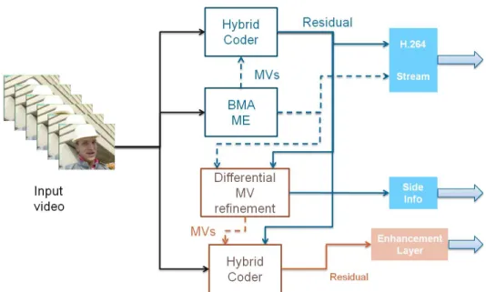
The CR+Res coding mode can be used to introduce quality scalability in a hybrid encoder. The concept is shown in Fig. 1. When a block is to be coded in Inter mode, the motion vector and the residual are produced and they constitute the regular stream. If the CR mode is used, the differential refinement of motion vector is performed. The encoder can compute the RD performance of the CR mode, and possibly it can choose to encode the macroblock as CR. In any case, it should send a further bit of side information, in order to signal to the decoder wheter the regular Inter mode or the CR mode have been used.

The regular residual, the Inter motion vector, and the side information contistute the base layer of this scalable encoder.

If the CR+Res mode is enabled, a further piece of information is generated by the encoder, that is the new residual related to the CR prediction. This residual (encoded as it is or as differnce with respect to the ordinary residual) constitutes the enhancement layer of the scalable codec.

One problem of this scalable codec is related to rate-distortion optimization. If the RD-optimization is activated, we do not know how many (if any) macroblocks will actually be encoded in CR mode (base layer) or in CR+Res mode. Therefore, we are

(12)

Figure 1: Scheme of a scalable video coder using the CR+Res mode in order to achieve quality scalability

not able to control the rate or the quality of the two layers. As a consequence, we need to impose stronger constraints on the two layers.

One possible solution is the following. We enforce all the macroblocks in a Inter layer to be coded with a temporal prediction mode. In other words we prevent Intra blocks in a P (or B) slice. Then, for all the macroblocks encoded in CR mode, we build an enhancement layer using the CR+Res mode. In this way the base layer is optimized, but this is no longer true for the enhancement layer. We call this solution base-optmized (BO) CR scalability A second possible solution is to keep the same base layer of the BO solution, and to encode all the enhancement macroblocks as CR+Res. We observe that it is always possible to add a CR+Res layer to a macroblock encoded with an Inter prediction mode. We call this solution all-CR enhancement (AE). A third possible solution is to perform the RD optimization using the λ value for the enhancement layer. In this optimization only Inter and CR+Res mode are in compe-tition (with all the possible parcompe-titions). In this way we build the enhancement layer. Then we discard the RRE information from the macroblocks encoded in CR+Res, thus generating the base layer. We call this solution enhancement-optimized CR scalability (EO).

We observe that, with these solutions, we still risk to have only a few blocks encoded in a CR mode (which is necessary to achieve scalability). Therefore we modify them in order to increase the number of macroblocks encoded with the CR mode.

A first modification consist in penalizing the non-CR modes in the mode selection procedure. This can be achieved by adding a constant Jpen(mode) to the cost function

(13)

of a generic mode. We set:

Jpen(Inter) = a (5)

Jpen(CR) = 0 (6)

Jpen(CR + Res) = 0 (7)

The value of a manages the trade-off betwee RD optimization and scalabiltiy. If a = 0 the mode selection is performed in the usual RD-optimized fashion, with the risk of having a few blocks (or no block) encoded in CR, with the consequence that the base and the enhancement layers are identical. On the other extreme, if a = +∞, all the macroblocks will be coded in a CR mode, allowing a scalable coding for each of them. However, preventing the inter mode for any MB could impair global RD performance. Intermediate values of a should allow a good degree of scalablity without affecting too much the RD performances. In other words, we will choose the CR mode a bit more often than in the regular case, but only if this does not increase too much the value of the cost function.

2.2 Intra prediction based on generalized template matching

Closed-loop intra prediction plays an important role in minimizing the encoded in-formation of an image or an intra frame in a video sequence. E.g., in H.264/AVC, there are two intra prediction types called Intra-16x16 and Intra-4x4 respectively [43]. The Intra-16x16 type supports four intra prediction modes while the Intra-4x4 type supports nine modes. Each 4x4 block is predicted from prior encoded samples from spatially neighboring blocks. In addition to the so-called “DC” mode which consists in predicting the entire 4x4 block from the mean of neighboring pixels, eight directional prediction modes are specified. The prediction is done by simply “propagating” the pixel values along the specified direction. This approach is suitable in presence of con-tours, when the directional mode chosen corresponds to the orientation of the contour. However, it fails in more complex textured areas.

An alternative spatial prediction algorithm based on template matching has been described in [31]. In this method, the block to be predicted of size 4x4 is further divided into four 2x2 sub-blocks. Template matching based prediction is conducted for each sub-block accordingly. The best candidate sub-block of size 2x2 is determined by minimizing the sum of absolute distance (SAD) between template and candidate neighborhood. The four best match candidate sub-blocks constitute the prediction of the block to be predicted. This approach has later been improved in [32] by averaging the multiple template matching predictors, including larger and directional templates, as a result of more than 15% coding efficiency in H.264/AVC. Any extensions and variations of this method are straightforward. In the experiments reported in this paper, 8x8 block size has been used without further dividing the block into sub-blocks. Here, a spatial prediction method based on sparse signal approximation (such as matching pursuits (MP) [19], orthogonal matching pursuits (OMP) [24], etc.) has been considered and assessed comparatively to the template matching based spatial prediction technique. The principle of the approach, as initially proposed in [36], is

(14)

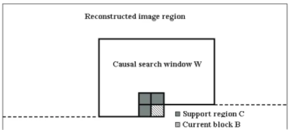
Figure 2: C is the approximation support (template), B is the current block to be predicted and W is the window from which texture patches are taken to construct the dictionary to be used for the prediction of B.

to first search for the linear combination of basis functions which best approximates known sample values in a causal neighborhood (template), and keep the same linear combination of basis functions to approximate the unknown sample values in the block to be predicted. Since a good representation of the template does not necessarily lead to a good approximation of the block to be predicted, the iteration number, which minimizes a chosen criterion, needs to be transmitted to the decoder. The considered criteria are the mean square error (MSE) of the predicted signal and a rate-distortion (RD) cost function when the prediction is used in a coding scheme.

Note that, this approach can be seen as an extension of the template matching based prediction (which keeps one basis function with a weighting coefficient equal to 1). In order to have a fair comparison with template matching, the sparse prediction algo-rithm is iterated only once. In the experiments reported here, the OMP algoalgo-rithm has been used by considering a locally adaptive dictionary as defined in [36]. In addition, both a static and MSE/RD optimized dynamic templates are used. The best approx-imation support (or template) among a set of seven pre-defined templates is selected according to the corresponding criterion, that is minimizing either the residual MSE or the RD cost function on the predicted block.

The proposed spatial prediction method has been assessed in a coding scheme in which the residue blocks are encoded with an algorithm similar to JPEG. The ap-proximation support type (if dynamic templates are used) is Huffman encoded. The prediction and coding PSNR/bit-rate performance curves show a gain up to 3 dB when compared with the conventional template matching based prediction.

2.2.1 Template matching and sparse prediction

Let S denote a region in the image containing a block B of n × n pixels and its causal neighborhood C used as approximation support (template) as shown in Fig. 2. The region S contains 4 blocks, hence of size N = 2n ×2n pixels, for running the prediction algorithm. In the region S, there are known values (the template C) and unknowns (the values of the pixels of the block B to be predicted). The principle of the prediction approach is to first search for the best approximation for the known values in C, and keep the same procedure to approximate the unknown pixel values in B.

(15)

Figure 3: Seven possible modes for approximation support (dynamic template) selec-tion. Mode 1 corresponds to the conventional static template.

The N sample values of the area S are stacked in a vector b. Let A be the corre-sponding dictionary for the prediction algorithm represented by a matrix of dimension N × M, where M ≥ N. The dictionary A is constructed by stacking the luminance values of all patches in a given causal search window W in the reconstructed image region as shown in Fig. 2. The use of a causal window guarantees that the decoder can construct the same dictionary.

2.2.2 Template matching (TM) based spatial prediction

Given A ∈ RN ×M and b ∈ RN, the template matching algorithm searches the best match between template and candidate sample values. The vector b is known as the template (also referred as the filter mask), and the matrix A is referred as the dictionary where its columns aj are the candidates. The candidates correspond to the

luminance values of texture patches extracted from the search window W .

The problem of template matching seeks a solution to minimization of a distance d as

arg min

j∈{1...M}{d

j: dj = DIST (b, aj)} .

Here, the operator DIST denotes a simple distance metric such as sum of squared distance (SSD), SAD, MSE, etc. The best match (minimum distance) candidate is assigned as the predictor of the template b.

Static template prediction

A static template is referred as the commonly used conventional template, i.e., mode 1 in Fig. 3. Let us suppose that the static template (mode 1) is used for prediction. For the first step, that is search for the best approximation of the known pixel values, the matrix A is modified by masking its rows corresponding to the spatial location of the pixels of the area B (the unknown pixel values). A compacted matrix Acof size 3n2× M is obtained. The known input image is compacted in the vector bc

(16)

Optimized dynamic templates

The optimum dynamic template is selected among seven pre-defined modes as shown in Fig. 3. The optimization is conducted according to two different criteria: 1. min-imization of the prediction residue MSE; 2. minmin-imization of the RD cost function J = D + λR, where D is the reconstructed block MSE (after adding the quantized residue when used in the coding scheme), and R is the residue coding cost estimated as R = γ0M& [18] with M& being defined as the number of non-zero quantized DCT

coefficients and γ0= 6.5.

2.2.3 Sparse approximation based spatial prediction

Given A ∈ RN ×M and b ∈ RN with N << M and A is of full rank, the problem of sparse approximation consists in seeking the solution of

min{"x"0 : Ax = b},

where "x"0 denotes the L0 norm of x, i.e., the number of non-zero components in x.

A is known as the dictionary, its columns aj are the atoms, they are assumed to be

normalized in Euclidean norm. There are many solutions x to Ax = b and the problem is to find the sparsest, i.e., the one for which x has the fewest non-zero components.

In practice, one actually seeks an approximate solution which satisfies: min{"x"0 : "Ax − b"p≤ ρ},

for some ρ ≥ 0, characterizing an admissible reconstruction error. The norm p is usually 2. Except for the exhaustive combinatorial approach, there is no known method to find the exact solution under general conditions on the dictionary A. Searching for this sparsest representation is hence computationally intractable. MP algorithms have been introduced as heuristic methods which aim at finding approximate solutions to the above problem with tractable complexity.

In the project, the OMP algorithm which offers an iterative optimal solution to the above problem is considered. It generates a sequence of M dimensional vectors xk

having an increasing number of non-zero components in the following way. At the first iteration x0 = 0 and an initial residual vector r0 = b − Ax0 = b is computed.

At iteration k, the algorithm identifies the atom ajk having the maximum correlation

(17)

selected in the previous iterations. One then projects b onto the subspace spanned by the columns of Ak, i.e., one solves

min

x "Ak

x_{− b"}2, and the coefficient vector at the kth iteration is given as

xk = (ATkAk)−1ATkb= A + kb,

where A+_k is the pseudo-inverse of Ak. Notice that here xkis a vector of coefficients. All

the coefficients assigned to the selected atoms are recomputed at each step. However, in the experiments reported here, only one iteration has been considered for the sake of comparison with template matching.

The principle of the prediction based on sparse approximation is to first search for a best basis function (atom) which best approximates the known values in C, and keep the same basis function and weighting coefficient to approximate the unknown pixel values in B.

Let the quantity x denote a vector which will contain the result of the sparse ap-proximation, i.e., the coefficient of the expansion of the vector b on only one atom. The sparse representation algorithm then proceeds by solving the approximate mini-mization

xopt= min

x "bc− Ac

x_"2₂ _{subject to "x"}0= 1.

To recover the extrapolated signal ˆb, the full matrix A is multiplied by xopt as ˆb=

Axopt.

Here, the columns (atoms) acj of the compacted dictionary Ac correspond to the

normalized luminance values of texture patches extracted from the search window W . 2.2.4 Linear combination of Template Matching predictors

In this variant of the prediction based on sparse approximation, in the search for the best approximation of the template, one searches for the K most correlated atoms and of their corresponding weight, each time with one iteration. One then computes an averable of the three resulting predictions.

2.3 Advances in intra-prediction coding based on texture

synthesis*

Some new ideas for improving the intra prediction methods were developed recently. They are desribed in details in the delivrable D2.2.

2.4 Adaptive WT and perceptual impact in image coding

Wavelet transform (WT) is a very useful tool for image processing and compression. In particular, the lifting scheme (LS) implementation of WT was originally introduced

(18)

Dynamic template OMP (26.48 dB/0.75 bpp)

Dynamic template TM (25.69 dB/0.85 bpp)

Static template OMP (24.23 dB/0.84 bpp)

Static template TM (23.97 dB/0.88 bpp) Figure 4: Prediction results of Foreman image.

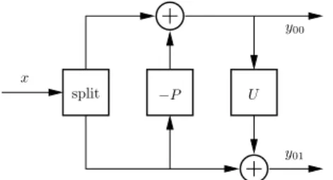
by Sweldens [30] to design wavelets on complex geometrical surfaces, but at the same time it offers a simple way to build up both classic wavelet transforms and new ones. The elements composing the lifting scheme are shown in Fig. 5. We call x the input signal, and yij the wavelet subbands. In particular, the first index determines the

decomposition level (i = 0 being the first one), and the second index discriminates the channel (j = 0 for the low-pass or approximation signal, j = 1 for the high pass or detail signal). The input signal x is split into its even and odd samples, respectively called the approximation and the detail signal. Then, a prediction operator P is used in order to predict the odd samples of x from a linear combination of even samples. The prediction is removed from the odd samples in order to reduce their correlation with the even ones. Finally for the third block, the update operator U is chosen in such a way that the approximation signal y00satisfies certain constraints, such as preserving

the average of the input or reducing aliasing. It is interesting to notice that, with a proper combination of lifting steps (prediction and update) it is possible to enhance a given transform by imposing new properties on the resulting decomposition (for example, more vanishing moments).

LS are very flexible while preserving the perfect reconstruction property, and this allows to replace linear filters by nonlinear ones. For example, LS with adaptive update [25] or adaptive prediction [10,20] have been proposed in the literature, with the

(19)

x

y00

y01

−P U

split

Figure 5: Lifting scheme with a single lifting stage

target of avoiding oversmoothing of object contours, and at the same time of exploiting the correlation of homogeneous regions by using long filters on them. The adaptivity makes it possible to use different filters over different parts of image. As a consequence, the resulting transform can be strongly non-isometric. This is a major problem for compression, since all most successful techniques rely on the distortion estimation in the transform domain, either explicitly like in EBCOT [33], or implicitly, like in the zero-tree based algorithms (EZW, SPIHT [26, 28]. Therefore, in order to efficiently use the adaptive lifting scheme for image compression, we need to estimate correctly the distortion from the transform coefficients. Usevitch showed that the energy of an uncorrelated signal (such as the quantization noise is supposed to be) can be estimated for generic linear wavelet filter banks [37]. We extended this approach to adaptive update LS (AULS) [22], and to adaptive prediction LS (APLS) [23] (in particular those inspired by the paper by Claypoole et al. [10]), obtaining satisfying results in term of distortion estimation and of rate-distortion (RD) performance improvement.

When non-isometric linear analysis is used, Usevitch [37] showed that the MSE in the original domain D is related to the MSE’s Dij of the wavelet subbands yij by

the linear relation D = )_ijwijDij. The weight wij is computed as norm of the

reconstruction polyphase matrix columns for subband yij.

However APLSs (as well as AULSs) are nonlinear systems, therefore no polyphase representation of them exist. Our contribution in previous papers [22, 23] was to extended this approach to adaptive LS, and to show how to compute the weights wij. The error D is still obtained as a weighted sum of the subband errors, but now

the weights depend on the input image, since the transform itself depends on it. In conclusion the proposed approach shows how to compute, in the transform domain, a metric which estimates the quantization noise MSE. This objective, non-perceptual distortion metric is then expressed as:

D1=

*

ij

wijdij (8)

where dij is the MSE in the subband ij:

dij =

*

n,m

(20)

compressed with an adaptive LS (with particular focus on APLS since they have by far the best performance). We make use of saliency maps in order to evaluate the different contributions of wavelet coefficients affecting different areas of the image; moreover we use the weights proposed in our previous works [23] in order to correctly compare different subbands.

We take inspiration from the quality metrics based on the saliency of specific areas in an image or a video. Let x be the original image, ˆx the distorted (or compressed) one, and n, m the spatial coordinates for pixels. The perceptual distortion is a weigthed sum of errors:

D2=

*

n,m

µ(n, m) [x(n, m) − ˆx(n, m)]p (10) where µ is a suitable saliency map. For example, in [9], it is proposed to take into account three phenomena: the image contrast (on a frame-by-frame basis), the global activity and the local activity (on a temporal basis). The image contrast mask, inspired on the work by Kutter and Winkler [16] uses a non-decimated WT of the image. Let WLL _{be the LL band of undecimated wavelet transform of x. The contrast saliency}

map is defined as:

α(n, m) = T [C0(n, m)] · WLL(n, m) (11) where T [C0] = + CT if C0< CM CT , C0 CM -" otherwise C0(n, m) = √ 2· · . |WHH_{(n, m)|}2_{+ |W}HL_{(n, m)|}2_{+ |W}LH_{(n, m)|}2 WLL_{(n, m)}

The parameters CT, CM, % can be assigned according to the observations made in

the paper [16]. This map does not take into account temporal effects in a video, and could be used if only fixed images are to be considered. However, one can make up for it by adding a further contribution accounting for global activity and based on motion vector norms.

In conclusion, we end up with a single masking function α which is higher where the observer is less sensible to errors, such that we can use µ = 1/α in Eq. (10).

The problem is that this distortion metric should be computed in the spatial domain, which is a quite large impairment for compression algorithms, as already noted in the first section.

(21)

2.4.2 Proposed metric

Based on the previous work [22, 23] and inspired on the perceptual metrics used in [9, 16], we propose a new metric which would allow to evaluate the perceptual effect of quantization (and actually of any other degradation) performed in the transformed domain. In other words, we want to make it possible to evaluate the perceptual quality of a compressed image directly from its transformed coefficients, when adaptive and highly non-linear transforms are used.

The proposed metric is based on subband energy weighting (to make it possible to use adaptive filters) and on the perceptual saliency described in the previous section. The weighting allows to compare wavelet subbands having different orientations and resolutions; the spatial masking allows to evaluate the impact of each WT coefficient according to the spatial region it will affect in the reconstructed image. However, since the different subbands have different resolutions, the mask α must be adapted to it. To this end, we define the mask value αi(n, m) at resolution level i as the average of

mask values in the positions associated to the coefficient (n, m):

αi(n, m) = 1 4i 2i_n+2i₋₁ * k=2i_n 2i_m+2i₋₁ * #=2im α(k, )) (12)

Now we can define the distortion evaluation in the transform domain. The new metric is similar to the one in Eq. (8):

D3=

*

ij

wijd&ij (13)

since the weights (computed as defined in [22,23]) are necessary to compare the distor-tion in different subbands. The innovadistor-tion stands in the term d&

ij, defined as follows: d& ij= * n,m µi(n, m) [yij(n, m) − ˆyij(n, m)]2 (14)

This equation is similar to the perceptual metric in Eq. (10); however here we use µi = 1/αi. In its turn, αi is defined in Eq. (12), and any saliency mask can be used in

principle, even though in a first moment we propose the one suggested in [9].

2.5 Examplar-based inpainting based on local geometry

2.5.1 Introduction

Inpainting methods play an important role in a wide range of applications. Removing text and advertisements (such as logos), removing undesired objects, noise reduc-tion [40] and image reconstrucreduc-tion from incomplete data are the key applicareduc-tions of inpainting methods. There are two algorithm categories: PDE (Partial Derivative Equation)-based schemes [35] and examplar-based schemes [11]. The former uses dif-fusion schemes in order to propagate structure in a given direction. The drawback is

(22)

order instead of field gradients. Second is to use a hierarchical approach to be less dependent on the singularities of local orientation. Third is related to constraining the template matching to search for best candidates in the isophote directions. Fourth is a K-nearest neighbor approach to compute the final candidate. The number K depends on the local context centered on the patch to be filled in.

This part is organized as follows. Section 2 describes the proposed method. Section 3 presents the performance of the method and a comparison with existing approaches. Some conclusions are dranw in this subsection.

2.5.2 Algorithm description

The goal of the proposed approach is to fill in the unknown areas of a picture I by using a patch-based method. As in [11], the inpainting is carried out in two steps: (i) determining the filling order; (ii) propagating the texture. We use almost the same notations as in [11]. They are briefly summarized below:

• the input picture noted I. Let I : Ω → Rn _{be a vector-valued data set and I} i

represents its i-th component;

• the source region noted ϕ, (ϕ = I − Ω); • the region to be filled noted Ω;

• a square block noted ψp, centered at the point p located near the front line.

The differences between the approach in [11] and the proposed one are on the one hand the use of structure tensors and in the other hand the use of a hierarchical approach. In the following, we first describe the algorithm for a unique level of the hierarchical decomposition and then we describe how the hierarchical approach is used.

For one level of the hierarchical decomposition

As previously mentioned, the proposed approach follows the approach in [11] int the way that the inpainting is made in two steps. In a first step, a filling priority is computed for each patch to be filled. The second step consists in looking for the best candidate to fill in the unknown areas in decreasing order of priority. These two steps are described in the following.

Computing patch priorities

Given a patch ψp centered at the point p (unknown pixel) located near the front

(23)

P (p) = C(p)D(p).

The first term, called the confidence, is the same as in [11]. It is given by: C(p) =

)

q∈ψp∩(I−Ω)C(q)

|ψp|

(15) where |ψp| is the area of ψp. This term is used to favor patches having the highest

number of known pixels (At the first iteration, C(p) = 1 ∀p ∈ Ω and C(p) = 0 ∀p ∈ I − Ω).

The second term, called the data term, is different from [11]. The definition of this term is inspired by PDE regularization methods acting on multivalued images [34]. The most efficient PDE-based schemes rely on the use of a structure tensor from which the local geometry can be computed. As the input is a multivalued image, the structure tensor, also called Di Zenzo matrix [13], is given by:

J=

n

*

i=1

∇Ii∇IiT (16)

J_{is the sum of the scalar structure tensors ∇I}i∇IiT of each image channel Ii(R,G,B).

The structure tensor gives information on orientation and magnitudes of structures of the image, as the gradient would do. However, as stated by Brox et al. [3], there are several advantages to use a structure tensor field rather than a gradient field. The tensor can be smoothed without cancellation effects : Jσ = J ∗ Gσ where

Gσ= _2πσ12exp(−

x2

+y2

2σ2 ), with standard deviation σ. In this paper, the standard

devi-ation of the Gaussian distribution is equal to 1.0.

The Gaussian convolution of the structure tensor provides more coherent local vec-tor geometry. This smoothing improves the robustness to noise and local orientation singularities. Another benefit of using a structure tensor is that a structure coher-ence indicator can be deduced from its eigenvalues. Based on the discrepancy of the eigenvalues, this kind of measure indicates the degree of anisotropy of a local region. The local vector geometry is computed from the structure tensor Jσ. Its eigenvectors

v1,2 (vi ∈ Rn) define an oriented orthogonal basis and its eigenvalues λ1,2 define the

amount of structure variation. v1 is the orientation with the highest fluctuations

(or-thogonal to the image contours), and v2 gives the preferred local orientation. This

eigenvector (having the smallest eigenvalue) indicates the isophote orientation. A data term D is then defined as [39]:

D(p) = α + (1 − α)exp(−_(λ C

1− λ2)2) (17)

where C is a positive value and α ∈ [0, 1] (C = 8 and α = 0.01). On flat regions (λ1 ≈ λ2), any direction is favored for the propagation (isotropic filling order). The

data term is important in presence of edges (λ1>> λ2).

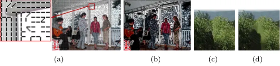
Figure 6 shows the isophote directions (a) and the value of the coherence norm (λ1−λ2

λ1+λ2)

2

(24)

Figure 6: (a) direction of the isophotes;(b) coherence norm: black areas correspond to areas for which there is no dominant direction; (c) Filling with the best candidate (K=1); (d) Filling with the best 10 candidates.

Propagating texture and structure information

Once the priority P has been computed for all unknown pixels p located near the front line, pixels are processed in decreasing order of priority. This filling order is called percentile priority-based concentric filling (PPCF). PPCF order is different from Criminisi’s approach. Criminisi et al. [11] updated the priority term after filling a patch and systematically used the pixel having the highest priority. The advantage is to propagate the structure throughout the hole to fill. However, this advantage is in a number of cases a weakness. Indeed, the risk, especially when the hole to fill is rather big, is to propagate too much the image structures. The PPCF approach allows us to start filling by the L% pixels having the highest priority. The propagation of image structures in the isophote direction is still preserved but to a lesser extent than in [11]. Once the pixel having the highest priority is found, a template matching based on the sum of squared differences (SSD) is applied to find a plausible candidate. SSD is computed between this candidate (entirely contained in ϕ) and the already filled or known pixels of ψp. Finally, the best candidate is chosen by the following formula:

ψq!= arg min ψq∈W

d(ψ!p, ψq) (18)

where d(., .) is the SSD. Note that a search window W centered on p is used to perform the matching.

Finding the best candidate is fundamental for different reasons. The filling process must ensure that there is a good matching between the known parts of ψpand a similar

patch in ϕ in order to fill the unknown parts of ψp. The metric used to evaluate the

similarity between patches is then important to propagate the texture and the structure in a coherent manner. Moreover, as the algorithm is iterative, the chosen candidate will influence significantly the result that will be obtained at the next iteration. An error leading to the apparition of a new structure can be propagated throughout the image. In order to improve the search for the best candidate, the previous strategy is modified as follows: ψq!= arg min ψq∈ϕ d(ψp!, ψq) + ( λ1− λ2 λ1+ λ2) 2 × f(p, q) (19)

(25)

where the first term d(., .) is still the SSD and the second term is used to favor candi-dates in the isophote direction, if any. Indeed, the term (λ1−λ2

λ1+λ2)

2 _{is a measure of the}

anisotropy at a given position (as explained in section 2.5.2). On flat areas, this term tends to 0. The function f (p, q) is given by:

f (p, q) = 1 % +|v2·vpq|

(vpq(

(20) where vpq is the vector between the centre p of patch ψp and the centre q of a

can-didate patch ψq. % is a small constant value, set to 0.001. If the vector vpq is not

collinear to the isophote direction (assessed by computing the scalar product v2· vpq),

this candidate is penalized. In the worst case (the two vectors are orthogonal), the penalization is equal to 1/%. When the two directions are collinear, the function f (p, q) tends to one.

A K nearest neighbour search algorithm is also used to compute the final candidate to improve the robustness. We follow Wexler et al.’s proposition [41] by taking into account that all candidate patches are not equally reliable (see equation 3 of [41]). An inpainting pixel !c is given by (ci are the pixels of the selected candidates):

!c = ) isici ) isi (21) where si is the similarity measure deduced from the distance (see equation 2 of [41]).

Most of the time, the number of candidates K is fixed. This solution is not well adapted. Indeed, on stochastic or fine textured regions, as soon as K is greater than one, the linear combination systematically induces blur. One solution to deal with that is to locally adapt the value K. In this approach we compute the variance σ2

W

on the window search. K is given by the function a +_1+σb2

W/T (in our implementation

we use a = 1, b = 9 and T = 100. It means that we can use up to 10 candidates to fill in the holes). Figure 6 (c) and (b) shows the rendering of a fine texture with the best and the best ten candidates. For this example, good rendering quality is achieved by taking into account only the best candidate.

Hierarchical decomposition

Previous sections described the proposed approach for a given pyramid level. One limitation concerns the computation of the gradient ∇I used to define the structure tensor. Indeed, as the pixels belonging to the hole to fill are initialized to a given value (0 for instance), it is required to compute the gradient only on the known part of the patch ψp. This constraint can undermine the final quality. To overcome this

limitation, a hierarchical decomposition is used in order to propagate throughout the pyramid levels an approximation of the structure tensor. A Gaussian pyramid is then built with successive low-pass filtering and downsampling by 2 in each dimension leading to nL levels. At the coarsest level L0, the algorithm described in the previous

section is applied. For a next pyramid level Ln, a linear combination between the

structure tensors of level Ln and Ln−1(after upsampling) is performed:

JLn

h = ν × J

(26)

salience and visual importance

We have already explained in the Chapter 4 of the D3.1 deliverable, how saliency maps can be used to drive decisions when coding images. This new study [38] aims at comparing two types of maps, obtained through psychophysical experiments.

Exactly two mechanisms of visual attention are at work when humans look at an image: bottom-up and top-down. Bottom-up refers to a mechanism driven by only low level features, such as color, luminance, contrast. Top-down refers to a mechanism which is more about to the meaning of the scene. According to these two mechanisms, the research about (bottom-up) visual saliency and (top-down) visual importance, which is also called ROI, can provide important insights into how biological visual systems address the image-analysis problem. However, despite the difference in the way visual salience and visual importance are determined in terms of visual process-ing, both salience and importance have traditionally been considered synonymous in the signal-processing community: They are both believed to denote the most visually "relevant" parts of the scene. In the study, we present the result of two psychophys-ical experiments and an associated computational analysis designed to quantify the relationship between visual salience and visual importance. In the first experiment, importance maps were collected by asking human subjects to rate the relative visual importance of each object within a database of hand-segmented images. In the sec-ond experiment, experimental saliency maps were computed from visual gaze pattern measured for these same images by using an eye-tracker and task-free viewing. The results of the experiment revealed that the relationship between visual salience and visual importance is strongest in the first two second of the 15-second observation in-terval, which implies that top-down mechanisms dominate eye movements during this period.From the psychophysical point of view, these results suggest a possible strategy for human visual coding. If the human visual system can so rapidly identify the main subject(s) in a scene, such information can be used to prime lower-level neurons to better encode the visual-level tasks such as scene categorization. Several researchers have suggested that rapid visual priming might be achieved via feedback and/or lat-eral interactions between groups of neurons after the "gist" of the scene is determined. The results of the study provide psychophysical evidence that lends support to a gist-based strategy and a possible role for the feedback connections that are so prevalent in mammalian visual systemsIn the study, we have attempted to quantify the similarities and differences between bottom-up visual salience and top-down visual importance. The implications of these initial findings for image processing are quite important. As we know, several algorithms have been published which can successfully predict gaze

(27)

patterns [17]. Our results suggest that these predicted patterns can be used to predict importance maps when coupled with a segmentation scheme. In turn, the importance maps can then be used to perform importance-based processing such as compression, auto-cropping, enhancement, unequal error protection, and quality assessment.

2.7 Taking into account the geometric distortion

An efficient estimation and encoding of motion/disparity information is a crucial step in 2D and 3D video codecs. In particular, the displacement information can be at the origin very rich, and therefore very costly to represent. For this reason, displacement information is always in some way degraded in order to be efficiently sent. In order to justify these affirmation one can think to the “original” or “actual” motion vector field2

as to a dense (i.e. one vector per pixel), infinite-precision (i.e. not limited to integer, half or quarter pixel) field. When we encode this field we degradate it:

• Using only one vector per block of pixel,

• Reducing the precision to integer, half or quarter pixel precision

Usually, this information degradation is performed in such a way to optimize a rate-distortion cost function. This is for example when the best macroblock partition is selected in H.264 with a RD-optimization approach [29,42]. In this traditional context, the mode selection procedure can be interpreted as an implicit segmentation of the motion vector field in which the shape of the objects is constrained by the partitions of the encoder (e.g. the 7 partition modes of H.264, [44]).

This operation can be seen in the following way. We are corrupting an “optimal” MVF in order to reduce the coding cost. The representation of this “corrupted” MVF is driven by a rate-distortion cost function: the mode which minimize the functional J = D + λR is choosen, where R is the coding rate and D is usually a quanity related to the MSE.

We notice that in this operation there is no consideration for the perceptual impact of corrupting motion vectors. The basic idea proposed here stems from the consideration that we should take into account what is the effect of changing motion vectors on the perceived quality of the reconstructed image.

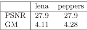
lena peppers PSNR 27.9 27.9

GM 4.11 4.28

Table 1: Geometrical distortion measure

At this end, we borrow the framework of geometric distortion estimation recently proposed by D’Angelo et al. [12]. In that paper, the authors introduced an objective perceptual and full-reference metric which allows to estimate the perceived quality of

2

For simplicity, we refer in the following to motion vectors, but all these considerations hold for disparity vectors as well

(28)

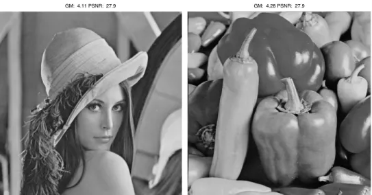
Figure 7: “Lena” and “peppers” after the same geometrical distortion. The left image is visibly corrupted (look at the vertical structure on the left), while the right one looks perfect. The PSNR is not able to catch the perceptual quality difference of these images, while the GM is, as shown in Table 1

an image affected by geometric distortion. The geometric distortion is represented as a MVF v applied to the original image X to give the distorted image Y

Y (p) = X(p + v)

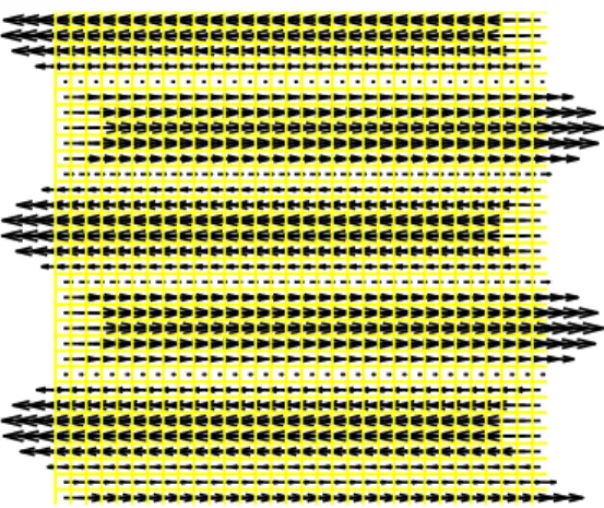
A couple of examples is shown in Fig. 7. The motion vector field is shown in Fig. 8. It amounts to only horizontal displacements, with a displacement amplitude varying along the vertical direction. We can argue that, even though the amplitude of the displacement field is exactly the same for the two images, the perceived quality is dif-ferent, since “lena” has much more vertical contours and structures that are disrupted by the horizontal shift of pixels. PSNR is unfit to catch the effect of geometrical dis-tortion. The metric proposed by D’Angelo et al. [12] seems better adapted to this end, as shown in Tab 1.

2.7.1 The original distortion measure

This metric (for short, GM, as for geometry-based metric) is based on computing the geometric features of the image directed along a given direction θ. Then, for each motion vector, authods consider its component along direction θ, be it vθ, and finally

the gradient of vθ in the direction orthogonal to θ. This gradient gives the amount

of degradation with respect to the structures alligned with θ; a Gabor filtering of the image allows to find the amount of energy of the structures having the same orientation θ for the considered pixel. Then, the degradation estimation takes into account both

(29)

Figure 8: The motion vector field used for generating the geometrical distortion

the displacement (gradient of vθin the direction orthogonal to θ) and the importance

of the structures (Gabor filter). A product of suitable real powers of these contribution assesses the geometrical estimation for a pixel and for a given direction. The global geometrical distortion measure is given by averaging over all directions and all pixels. Tests show that considering two directions, horizontal and vertical, is already sufficient for collecting the most of the relevant information.

2.7.2 Proposed methodology

The proposed methodology is based on the following assumption: there is some optimal dense motion vector field, and we are able to estimate it3

. Let v∗ _{be this MVF. Every}

time we do not use this MVf it is like we are imposing a geometrical distortion through an error field δv:

δv = v∗_{− v,}

where v is the MVF we are actually using. Therefore we can change the cost function of v, from

J(v) = D(v) + λR(v) to

J(v) = GM (δv) + λR(v)

. Finally we can try to use this new cost function whenever the old one was used: • Motion estimation

• Motion vector encoding • Mode selection

3

(30)

We observe that the proposed metric lends itself well to the considered framework. In particular, it suggests the use of a closed-loop, two-passes encoder.

• This metric is a full reference one, which perfectly matches the closed-loop video encoding paradigm.

• It demands a pre-analysis of images, then providing a map of relevant struc-tures (according to some orientation). This also fit well with a two-passes video encoder, which in a first pass produce the information of all relevant oriented structures, and then, using these maps, can estimate the perceptual impact of motion/disparity information encoding.

In conclusion, the methodology proposed in this report is promising since it goes in the direction of assessing the perceptual effect of information degradation due to motion information compression. A perceptual encoder must take this phenomenon into account in order to perform an optimal rate-quality trade-off.

(31)

3 Performance evaluation

3.1 Dense motion vector estimation with Cafforio-Rocca

Algorithm

We considered several video sequences with different motion content, (from low motion content to irregular, high motion sequences) and we performed two kind of experiments on them. In a first set of experiments, described in section 3.1.1, we only considered the effectiveness of CR motion vector improvement in the framework of the H.264 codec. In the second set of experiments, described in section 3.1.4, we considered the introduction of the CRA within the H.264 codec, and we evaluated the RD performances with respect to the variations of all relevant parameters.

3.1.1 Tests on Motion Estimation

In this section we consider tests made with the goal of validating the CR ME. We will not consider the impact over the global RD performances of the encoder.

3.1.2 Comparison with a Block Matching Algorithm

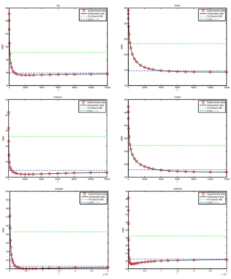
In a first set of experiments we compared the CR MVs with a MVF obtained by classical block-matching algorithms. We considered several input video sequences, and for each of them several pairs of current-reference frames (not necessarily consecutive images). For each pair of current-reference images, we computed the prediction error energy with respect to the full-search BMA MVF, and the prediction error energy in the case of CR ME. In this case we use the original (i.e. not quantized images), and the computation has been repeated for several values of the Lagrangian parameter λ.

The results are shown in Fig. 9. For all the test sequences we find a similar behavior: but for very small values of λ, the CR vectors guarantee a better prediction with respect of the BMA (green dashed line). For increasing values of λ the MSE decreases quickly, reaches a minimum and then increases very slowly towards a limit value, corresponding to λ = ∞. The latter case corresponds to a null refinement: all the improvement is due to the validation test, and corresponds with difference between the green and blue dashed lines in Fig. 9. The minimum value of the MSE is obtained when besides the validation test, the vectors are modified by the refinement step. We also remark that the CRA is quite robust wrt the choice of λ; the difference between the minimum and the asymptotical value of the black curve is the contribution of the refinement step. 3.1.3 Motion estimation with quantized images

The first experiment shows us that the CRA has the potential to improve the BMA motion vectors. However comparing only the prediction MSE is not fair since the cost of encoding the vectors is not taken into account. Of course, in this case, it would be extremely costly to encode the CR vectors, since there is a vector per pixel. The RD comparison would be definitely favorable to the classical ME algorithm. This is however why the CRA is not used in hybrid video coders at least in its classical form.

(32)

0 2000 4000 6000 8000 10000 12000 40 60 80 100 120 λ MSE 0 2000 4000 6000 8000 10000 12000 100 150 200 250 λ MSE 0 2000 4000 6000 8000 10000 12000 30 35 40 45 50 55 λ MSE foreman Experimental data Interpolated data Full Search ME Limit λ → ∞ 0 2000 4000 6000 8000 10000 12000 150 200 250 300 350 400 450 λ MSE mobile Experimental data Interpolated data Full Search ME Limit λ → ∞ 0 0.5 1 1.5 2 2.5 3 x 104 110 120 130 140 150 160 170 180 190 200 λ MSE tempete Experimental data Interpolated data Full Search ME Limit λ → ∞ 0 0.5 1 1.5 2 2.5 3 x 104 20 22 24 26 28 30 32 34 36 38 40 λ MSE waterfall Experimental data Interpolated data Full Search ME Limit λ → ∞

(33)

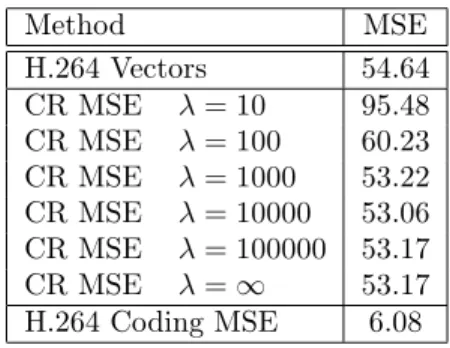
Method MSE H.264 Vectors 54.64 CR MSE λ = 10 95.48 CR MSE λ = 100 60.23 CR MSE λ = 1000 53.22 CR MSE λ = 10000 53.06 CR MSE λ = 100000 53.17 CR MSE λ = ∞ 53.17 H.264 Coding MSE 6.08

Table 2: Prediction error energy, “foreman” sequence.

Method MSE H.264 vectors 90.79 CR λ = 10 571.02 CR λ = 100 237.34 CR λ = 1000 92.09 CR λ = 10000 72.86 CR λ = 100000 71.68 CR λ = ∞ 71.69 H.264 MSE 3.49

Table 3: Prediction error energy, “mobile” sequence.

On the contrary, the in the modified CRA the cost of MV coding is zero, but this is obtained by sacrificing the accuracy of validation and refinement, which must be performed using quantized data.

We designed the a second kind of tests in order to evaluate the potential gains of the CRA in the framework of a H.264-like coder. Unlike the previous case, we did not used the original images to perform the CRA, but we used those available to a H.264 decoder. More precisely, we first used H.264 to produce: the MVF between two images in a video sequence (indicated by v, and the decoded current and reference image, indicated as ˆIk and ˆIh (e.g. h = k − 1).

Then the following quantities were computed:

H.264 Vectors MSE : The prediction error mean squared value for the H.264 vectors. vCR : The CR motion vectors, obtained by using ˆIk and ˆIh and v.

CR MSE : The prediction error mean squared value for the CR vectors.

Some results are summarized in table 2 and 3. We performed the same test over many other sequences, and we obtained similar results.

We observe that in this case as well, the CR method is able to potentially improve the performance: the prediction produced with the CR vectors has (but for small λ

(34)

tempete 0.01 -0.13%

Table 4: Rate distortion performances improvement when introducing the new coding mode into H.264.

values) a smaller error than the original H.264 vectors, even if the CRA is run over quantized images. Moreover in this case the comparison is fair in the sense that the CR vectors do not cost any bit more than the original ones.

The last line of the table reports the MSE of the decoded macroblock in H.264. Of course it is much smaller of the prediction error energy, since it benefits from the encoded residual information. As a conclusion, it is critical to keep an efficient residual coding, since it is responsible for a large amount of the distortion reduction.

3.1.4 RD performances

In this section we comment about the performance of the modified H.264 coder. In order to assess the effectiveness of the proposed method, we have implemented it within the JM H.264 codec. We considered several design choice: the effects of the Lagrangian parameter, of the threshold and of the initialization method. Finally we compare the RD comparison to the original H.264 coder.

The proposed method seems not to be too affected by the value of the threshold γ provided that it is not too small (usually γ > 10 works well). For the sake of brevity we do not report here all the experimental results. Likewise, we found that setting λ = 104_{works fairly well in all the test sequences. In the following, these values of the}

parameters are kept.

A larger impact on the performance is due to the validation step. Introducing a third candidate vector for validation allows a fast motion vector recover when passing from one object to another within the same block.

Finally we compared an H.264 coder where the new coding mode was implemented with the original one. The results are shown in table 4, where we report, for each test sequence, the improvement in PSNR and the bit-rate reduction computed with the Bjöntegard metric [2] over four QP values. We observe that the improvement are quite small, in part because the CR mode is rarely selected rarely (usually only for 10% of the blocks).

It is worth noting that the coding time with the modified coder are very close to those of the original one: we usually observed an increase less than 2%.