Optimal Yaw Rate Control for Over-Actuated Vehicles

(1)

HAL Id: hal-02525997

https://hal.archives-ouvertes.fr/hal-02525997

Submitted on 2 Apr 2020

HAL is a multi-disciplinary open access

archive for the deposit and dissemination of

sci-entific research documents, whether they are

pub-lished or not. The documents may come from

teaching and research institutions in France or

abroad, or from public or private research centers.

L’archive ouverte pluridisciplinaire HAL, est

destinée au dépôt et à la diffusion de documents

scientifiques de niveau recherche, publiés ou non,

émanant des établissements d’enseignement et de

recherche français ou étrangers, des laboratoires

publics ou privés.

Optimal Yaw Rate Control for Over-Actuated Vehicles

Moad Kissai, Bruno Monsuez, Adriana Tapus, Xavier Mouton, Didier

Martinez

To cite this version:

Moad Kissai, Bruno Monsuez, Adriana Tapus, Xavier Mouton, Didier Martinez. Optimal Yaw Rate

Control for Over-Actuated Vehicles. WCX SAE World Congress Experience, Apr 2020, Detroit,

United States. �hal-02525997�

(2)

Page 1 of 10

2020-01-1002

Optimal Yaw Rate Control for Over-Actuated Vehicles

Moad Kissai, Bruno Monsuez, Adriana Tapus

ENSTA Paris

Xavier Mouton, Didier Martinez

Group Renault

Abstract

As we are heading towards autonomous vehicles, additional driver assistance systems are being added. The vehicle motion is automated step by step to ensure passengers’ safety and comfort, while still preserving vehicle performance. However, simultaneous activations of concurrent systems may conflict, and non-suitable behavior may emerge. Our research work consists in proving that with the right coordination approach, simultaneous operation of different systems improve the vehicle’s performance and avoid the emergence of unwanted conflicts. To prove this, we gathered different control architectures implemented in commercial passenger cars, and we compared them with our control architecture using a unified reference vehicle model. The high-fidelity vehicle model is developed in Simcenter Amesim in a modular and extensible manner. This enables adding systems in a plug-and-play way. Not only different control architectures can be tested on the same vehicle, but also different systems combinations can be evaluated. In this research, the vehicle can steer at the front and at the rear, and each wheel can be braked independently. Each of the actuators concerned can influence the vehicle’s yaw rate leading in some cases in system conflicts. More complex control strategies are then implemented in Matlab/Simulink, and co-simulations are carried between both softwares in order to provide realistic results. It has been shown that optimal control allocation algorithms are more suitable to coordinate systems in an over-actuated vehicle. Moreover, if the optimization objectives are well formalized, performance, safety and comfort can be improved since the vehicle can benefit from the systems’ synergies.

Introduction

Future vehicles will probably be autonomous, or at least highly automated. Most of car manufacturers and equipment suppliers are investigating autonomous technologies in order to make the vehicles safer, more comfortable and more performant. An autonomous vehicle should be able to operate without or with a minimal supervision of a human. This particular aspect would induce huge changes in the automotive sector, especially from a control engineering perspective. Up to now, the human driver is the “controller” that closes the control loop to cope with any external disturbance. Not only that, the human is capable of learning and adapting his/her driving style especially in simultaneous operations. For example, thanks to a Lane Keeping Assistance (LKA) system [1], the vehicle can be enforced to stay within the limits of the road lanes.

However, the system does not manage the interactions between lateral and longitudinal dynamics at the entry, within and at the exit of a cornering. A supervisory strategy should be ensured when two or more systems have to be activated since longitudinal and lateral dynamics are coupled [2]. Today, this supervisor is the human driver. For autonomous vehicles, not only the control loop should be closed in order to cope with external disturbances, but also an optimal distribution strategy should be ensured to supervise the coupled systems. Taking away the human driver from the steering wheel and the acceleration/braking pedals, adds various complexities to the control algorithms. Today’s vehicles are over-actuated where each system is developed for a specific feature. This over-actuation is expected to grow going towards autonomous vehicles. Without any coordination strategy or a human supervisor, conflicts may be induced between the interactive systems, particularly when these systems are acting on the same physical variable. For example, the Renault Talisman is equipped with both a 4-Wheel Steering (4WS) system [3] and a braking-based Vehicle Dynamics Control (VDC) system [4]. The 4WS system generates a rear steering angle which creates a rear lateral tire force. This creates a yaw moment and therefore act on the yaw rate of the vehicle. But even if the VDC system is a braking-based one, this system is able to generate braking forces at only the right or the left wheels of the vehicle. This also can create a yaw moment and act on the yaw rate of the vehicle. In today’s automotive industry, when a similar situation is encountered, downstream coordination strategies are adopted [5],[6]. Since each system is developed independently by a different supplier, and provided most of the time in a black-box, the car manufacturer use only a prioritization strategy to avoid any conflict. One system is then activated at a time, and the couplings are managed by the human driver. Nowadays, we can find two types of assistance systems: systems in an open-loop control strategy only, and systems in a closed one. Assistance systems as the 4WS system are actually implemented by car manufacturers in an open-loop using feedforward controllers [7], [8]. Even though, several efforts have been deployed to close the loop [9]-[11], to the best of our knowledge, few technological issues, particularly regarding communication delays and sensors noises, still inhibit car manufacturers to adopt a closed loop architecture. Whether the control system is in an open-loop or in a closed one, we have noticed that prioritization strategy is still adopted to coordinate several systems in an over-actuated passenger cars.

The prioritization strategies not only limit the real potential of the car by activating one system at a time, but they are especially not suitable for autonomous vehicles. If we take again the case of the LKA in a

(3)

Page 2 of 10

cornering maneuver, the autonomous vehicle should be able to stay within the limits of the lane and at the same time decelerate at the entry of the cornering and accelerate at its exit. Activating one system at a time would no longer be sufficient, and systems’ interactions should be taken into account. Vehicle dynamics couplings, especially at the tire level have been most of the time neglected [5]. As the human is the high-level supervisor, assistance systems use to focus on controlling only one specific dynamic. This is about to change with the emergence of autonomous vehicles. Vehicle dynamics couplings and systems interactions can no longer be neglected, and smarter coordination strategies should be adopted. Through several previous works [12],[13], it was shown that optimization-based control allocation algorithms are most likely to solve this problem. These algorithms take into account the effectiveness of each effector in real-time to generate the best effort distribution depending on the chosen objectives: usually the safety objective is given a higher weight than a comfort objective. In the control allocation framework, systems interactions are expressly formulated. For good measure, a high-level controller takes into account the vehicle dynamics couplings, and the couplings of tire dynamics through the friction ellipse [13] are taken into account as constraints in the optimal distribution problem. In this way, several systems can be activated at the same time and ensure an optimal global vehicle motion control. The purpose of this paper is to provide to the industry practioners a clear roadmap for future global chassis control systems. We will start by a real passenger car control strategy in an open loop to show that this will not be sufficient for future autonomous cars. We will then show the purpose of closing the loop. And finally we will demonstrate the need of optimal control allocation strategy to improve the vehicle’s performance and the passengers’ safety and comfort. A co-simulation procedure is adopted to provide realistic results. All the control strategies are implement in Matlab/Simulink®_,

while a common high-fidelity modular vehicle model is developed in Simcenter Amesim®_{to serve as a comparison platform for the}

different strategies. Future industrial challenges are also discussed and conclusions are outlined.

High-Fidelity Vehicle Model Description

We first start by describing the common vehicle model used for comparing the different control strategies. The vehicle model represents the new Renault Talisman equipped with a 4WS system and a braking-based VDC system. These two systems serve as an assistance system to control the vehicle’s yaw rate and manage the lateral dynamics. The vehicle’s chassis is exploded to make it modular and extensible. Not only different control strategies can be tested, but also additional chassis systems and Advanced Driver Assistance Systems (ADAS) can be added to evaluate the benefits of each system.

Simcenter Amesim

®

Amesim stands for Advanced Modeling Environment for

performing Simulations of engineering systems. It is based on an intuitive graphical interface in which the system is displayed throughout the simulation process. This interface provides several automotive components that can be tuned both analytically and empirically to make the model as close as possible to the real vehicle dynamics. For example, Pacejka equations [13] can be adopted to model the tire dynamics, but empirical tables are adopted to model the elastokinematic model that computes the elastic displacement of the wheel (elastic displacement of wheel center and elastic angular

displacement of the rim plane) under axle system constraint forces. In this way, the vehicle model is made as close as possible from the real vehicle without any control strategy.

Renault Talisman

Model

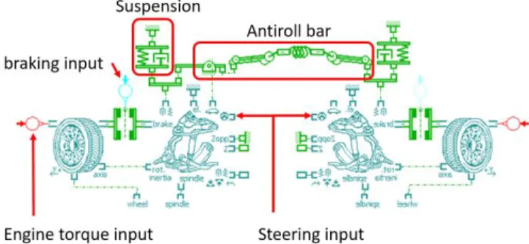
A 4-wheel steering chassis is modeled in our case. Each axle is modeled as Figure 1 shows.

Figure 1. Front axle modeling in Amesim with engine and braking torques inputs, steering input, suspensions and antiroll bar.

In our case, the same engine torque is applied to both front wheels as the Talisman by one conventional engine. However, torque vectoring systems can be easily implemented in this modular chassis. Here, no engine torques inputs are applied to the rear axle. Braking inputs differ from right to left wheels in order to apply VDC control strategy. The steering input corresponds to the front steering wheel angle. The 4WS system acts on the rear axle. Finally, a suspended mass is added above the chassis and linked through the suspensions.

Inputs/Outputs

The inputs to the vehicle model are: front steering wheel angle (provided by a human driver or computed by an autopilot system (Figure 2)), speed profile target, rear steering angle request, front-left braking torque request, front-right braking torque request, rear-left braking torque request, rear-right braking torque request. These requests come from the different control strategies implemented in Matlab/Simulink®_.

Figure 2. Front steering system modeling in Amesim.

The outputs are the different measurable dynamics of the vehicle: the vehicle’s yaw rate that can be measured by a gyroscope, the longitudinal and the lateral accelerations that can be measured by an Inertial Measurement Unit (IMU), and the effective rear steering angle provided by the 4WS system. These signals are then fed to Matlab in case of a closed-loop control in the co-simulation process.

(4)

Page 3 of 10

The VDC System

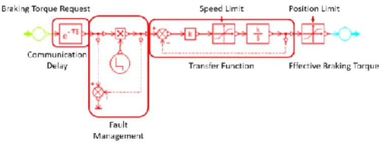
The braking torque can be applied thanks to a rotary friction torque generator as shown in Figure 1. Nevertheless, an additional transfer function is added between the braking request and the effective braking torque to better represent the dynamics of the braking actuator.

Figure 3. Modeling of braking dynamics in Amesim.

A similar transfer function is implement for the 4WS system. The braking torque distribution is managed by the corresponding control strategy.

The 4WS System

The rear steering angle is generated through a pneumatic system. The request is provided electronically to the 4WS system. The pneumatic system moves then a piston to move both rear wheels (Figure 4).

Figure 4. Rear steering system modeling in Amesim. The validation of the model is detailed in [9].

Today’s Open Loop Strategies

As long as a human driver still supervises the vehicle, external disturbances can be managed by him/her. With the technological complexity that the a closed-loop brings in terms of communication delays and noises propagation, car manufacturers still favor simpler strategies by tuning open-loop strategies. The strategy consists on following a desired reference vehicle model. In the case of the Renault Talisman, the reference model consists of a tuned yaw rate

reference generator. A reference model is tuned, and the rear steering angle is computed to add the additional yaw moment needed to reach the desired behavior. The VDC system is activated if a fault is detected in the 4WS system, or if this latter get saturated. The braking torques are also generated in order to add the additional yaw moment needed to reach the desired dynamics.

Yaw Rate Reference

As in our case, only the lateral dynamics need to be controlled, a bicycle model is usually adopted [16] as shown in Figure 5. The bicycle model can be considered as an ideal behavior to follow when it is well tuned: a neutral behavior should be ensured rather than an oversteering or understeering one. Indeed, the vehicle’s behavior should be predictable. If a human driver is controlling the vehicle, a slightly understeering behavior can be allowed, since drivers can recover the vehicle in this case. Whether the vehicle is autonomous or not, an oversteering behavior should definitely be avoided, because a counter-steering maneuver may easily lead to the loss of

controllability of the vehicle. This yaw rate reference can be further tuned to generate different motion feelings, e.g. sportive mode, comfort mode and so on.

Figure 5. The bicycle model.

As Figure 5 shows, the bicycle consists of considering one equivalent wheel at each axle since only one steering angle is generated by axle. Only the linear behavior of the tire is considered which gives the following equations: {𝐹𝑦𝑓= 𝐶𝛼𝑓𝛼𝑓 𝐹𝑦𝑟= 𝐶𝛼𝑟𝛼𝑟 (1) (2) With:

 𝐹𝑦𝑖 : equivalent lateral tire force at the i

th_{axle, with i=f for}

front or r for rear,

 𝐶𝛼𝑖 : equivalent cornering stiffness of the i

th_axle,

 𝛼𝑖 : equivalent side-slip of the ith axle.

The side-slips are expressed as follows:

{ 𝛼_𝑓= 𝛿𝑓− 𝑉𝑦+ 𝜓̇𝑙𝑓 𝑉𝑥 𝛼𝑟= 𝛿𝑟− 𝑉𝑦− 𝜓̇𝑙𝑟 𝑉𝑥

(5)

Page 4 of 10

(3) (4) With:

 𝛿𝑓 : the front steering angle,

 𝛿𝑟 : the rear steering angle,

 𝑙𝑓 : distance between the front axle and the vehicle’s Center of

Gravity (CoG),

 𝑙𝑟 : distance between the rear axle and the vehicle’s CoG,

 𝑉𝑥 : the vehicle’s longitudinal speed,

 𝑉𝑦 : the vehicle’s lateral speed,

 𝜓̇ : the vehicle’s yaw rate.

The equations of motion are determined by using Newton’s second law of motion: {𝑀(𝑉̇𝑦+ 𝜓̇𝑉𝑥) = 𝐹𝑦𝑓+ 𝐹𝑦𝑟 𝐼𝑧𝜓̈ = 𝐹𝑦𝑓𝑙𝑓− 𝐹𝑦𝑟𝑙𝑟 (5) (6) With:

 𝑀 : the vehicle’s global mass,  𝐼𝑧 : the vehicle’s yaw inertia moment.

The vehicle is usually designed to exhibit a neutral behavior. However, due to parameters and dynamics uncertainties, automotive engineers tend to adopt few safety margins, and design an

understeering vehicle. Indeed, an understeering vehicle is still better than an oversteering one, since this latter scares easily the driver, and may induce some unexpected maneuvers and destabilize the vehicle. The role of a 4WS steering system is then to help the driver achieve a neutral behavior, or if the driver wishes, a more sportive behavior. The reference model is then a transfer function between 𝛿𝑓 and 𝜓̇ in

case of a neutral behavior. If the real parameters of the vehicle do not exhibit a neutral behavior, a 𝛿𝑟 is added to achieve this behavior.

This is generally designed through several experimentations. From equations (1)-(6) we can deduce the static transfer function between 𝛿𝑓 and 𝜓̇: 𝜓̇𝑟𝑒𝑓= 𝑇𝛿𝑓→𝜓̇(0)𝛿𝑓= 𝑉𝑥 𝐿 + (_𝐶𝑙𝑟 𝛼𝑓 −_𝐶𝑙𝑓 𝛼𝑟 )𝑀𝑉𝑥2 𝐿 𝛿𝑓 (7) A saturation should be also added to this reference, as the steady-state yaw rate response cannot exceed a maximum achievable value of [17]:

𝜓̇𝑚𝑎𝑥≈ 𝜇

𝑔 𝑉𝑥

(8) With 𝑔 is the standard acceleration due to gravity and 𝜇 is the friction coefficient that expresses the quality of the contact between the tire and the road.

The 4WS Control Strategy

The control strategy is based on Ackermann steering geometry [18]. At a low speed, the Figure 6 is considered.

Figure 6. Steering geometry at a low speed. In this case, we can write:

tan 𝛿𝑓=

𝐿 𝑅

(9) Where 𝐿 = 𝑙𝑓+ 𝑙𝑟 is the vehicle’s wheelbase, and 𝑅 the radius of the

trajectory’s curvature. In contrast, at high velocities, the Figure 7 should be rather considered.

Figure 6. Steering geometry at a high speed. In this case:

tan(𝛿) =𝐿

𝑅+ 𝛼𝑓− 𝛼𝑟

(10) By considering also a stationary cornering, we can write:

𝑀𝑉

2

𝑅 = 𝐹𝑦𝑓+ 𝐹𝑦𝑟

(11) This gives:

(6)

Page 5 of 10 𝛿 =𝐿 𝑅+ ( 𝑀𝑙𝑟 𝐶𝛼𝑓𝐿 −𝑀𝑙𝑓 𝐶𝛼𝑟𝐿 )𝑉 2 𝑅 = 𝐿 𝑅+ 𝐾𝑢𝑔 𝑉2 𝑅 (12) 𝐾𝑢𝑔= 𝑀𝑙𝑟 𝐶_𝛼𝑓𝐿− 𝑀𝑙𝑓

𝐶𝛼𝑟𝐿 is defined as the understeer gradient [19]:

 If 𝐾𝑢𝑔= 0 ⇒ 𝐶𝛼𝑓𝑙𝑓= 𝐶𝛼𝑟𝑙𝑟 : both axles have the same guiding

potential, and we recover the neutral behavior where 𝛿 =𝐿

𝑅.

 If 𝐾𝑢𝑔> 0 ⇒ 𝐶𝛼𝑓𝑙𝑓< 𝐶𝛼𝑟𝑙𝑟 : the rear axle has a bigger guiding

potential, and the vehicle understeers.

 If 𝐾𝑢𝑔< 0 ⇒ 𝐶𝛼𝑓𝑙𝑓> 𝐶𝛼𝑟𝑙𝑟 : the front axle has a bigger guiding

potential, and the vehicle oversteers.

The same parameter can be found in the yaw rate reference:

𝜓̇𝑟𝑒𝑓= 𝑉𝑥 𝐿 + (𝑙𝑟 𝐶𝛼𝑓 −_𝐶𝑙𝑓 𝛼𝑟 )𝑀𝑉𝑥2 𝐿 𝛿𝑓= 𝑉𝑥 𝐿 + 𝐾𝑢𝑔𝑉𝑥2 𝛿𝑓 (13) Therefore, by tuning 𝐾𝑢𝑔, we can impose a neutral, understeering or

oversteering behavior. Let us consider for example a desired neutral behavior, and let us consider that the vehicle does not exhibit a neutral behavior. We have in this case:

{ 𝜓̇𝑟𝑒𝑓= 𝑉𝑥 𝐿𝛿𝑓 𝜓̇𝑟𝑒𝑎𝑙= 𝑉𝑥 𝐿 + (_𝐶𝑙𝑟 𝛼𝑓 −_𝐶𝑙𝑓 𝛼𝑟 )𝑀𝑉𝑥2 𝐿 𝛿𝑓− 𝑉𝑥 𝐿 + (_𝐶𝑙𝑟 𝛼𝑓 −_𝐶𝑙𝑓 𝛼𝑟 )𝑀𝑉𝑥2 𝐿 𝛿𝑟 (14) (15) Therefore, in order to impose a neutral behavior, we should get

𝑉𝑥 𝐿𝛿𝑓= 𝑉𝑥 𝐿 + (_𝐶𝑙𝑟 𝛼𝑓 −_𝐶𝑙𝑓 𝛼𝑟 )𝑀𝑉𝑥2 𝐿 𝛿𝑓− 𝑉𝑥 𝐿 + (_𝐶𝑙𝑟 𝛼𝑓 −_𝐶𝑙𝑓 𝛼𝑟 )𝑀𝑉𝑥2 𝐿 𝛿𝑟 ⇒ 1 1 + (𝑙𝑟 𝐶𝛼𝑓 −_𝐶𝑙𝑓 𝛼𝑟 )𝑀𝑉𝑥2 𝐿2 𝛿𝑟= 1 1 + (𝑙𝑟 𝐶𝛼𝑓 −_𝐶𝑙𝑓 𝛼𝑟 )𝑀𝑉𝑥2 𝐿2 𝛿𝑓− 𝛿𝑓 ⇒ 𝛿𝑟= 𝛿𝑓− (1 + ( 𝑙𝑟 𝐶𝛼𝑓 − 𝑙𝑓 𝐶𝛼𝑟 )𝑀𝑉𝑥 2 𝐿2 ) 𝛿𝑓 ⇒ 𝛿𝑟= − ( 𝑙𝑟 𝐶𝛼𝑓 − 𝑙𝑓 𝐶𝛼𝑟 )𝑀𝑉𝑥 2 𝐿2 𝛿𝑓 (16) Equation (16) represents then the open-loop control strategy in the case of a neutral desired behavior. The strategy consists on considering the front steering angle and the speed as inputs and generating a rear steering angle according to equation (16). The same

methodology is used to generate a comfortable mode by choosing a 𝐾𝑢𝑔> 0, or a sportive mode by choosing 𝐾𝑢𝑔< 0. The different

behaviors can be robustly exhibited if the vehicle’s parameters are well identified and do not vary.

The VDC Control Strategy

The same methodology can be adopted in the case of the VDC by considering the corresponding transfer function. In this case, when the VDC is activated, the 4WS does not, so we have :

𝜓̇𝑟𝑒𝑎𝑙= 𝑉𝑥 𝐿 + (𝑙𝑟 𝐶𝛼𝑓 −_𝐶𝑙𝑓 𝛼𝑟 )𝑀𝑉𝑥2 𝐿 𝛿𝑓+ 𝑉𝑥(𝐶𝛼𝑓+ 𝐶𝛼𝑟) 𝐿𝐶𝛼𝑓𝐶𝛼𝑟 𝐿 + (𝑙𝑟 𝐶𝛼𝑓 −_𝐶𝑙𝑓 𝛼𝑟 )𝑀𝑉𝑥2 𝐿 𝑀𝑉𝐷𝐶 (17) With 𝑀𝑉𝐷𝐶 is the required additional yaw moment provided by the

VDC in order to reach the desired vehicle behavior. For a neutral behavior for example, the open-loop control law should be:

𝑀𝑉𝐷𝐶= (𝑙𝑟 𝐶𝛼𝑓 −_𝐶𝑙𝑓 𝛼𝑟 )𝑀𝑉𝑥2 𝐿2 (𝐶𝛼𝑓+ 𝐶𝛼𝑟) 𝐿𝐶𝛼𝑓𝐶𝛼𝑟 𝛿𝑓 (18) If 𝑀𝑉𝐷𝐶> 0, we activate only the left braking torques, and

vice-versa. The distribution between front and rear torques depend on the vertical load distribution [20]. For example, in case of 𝑀𝑉𝐷𝐶> 0:

{ 𝐶𝑏𝑓𝑙= 𝑅𝑑𝑦𝑛𝐹𝑥𝑓𝑙= 𝑅𝑑𝑦𝑛( 𝑙𝑟 𝐿− 𝑎𝑥 𝑔 ℎ 𝐿) 𝑀𝑉𝐷𝐶 𝑡 2 𝐶𝑏𝑟𝑙= 𝑅𝑑𝑦𝑛𝐹𝑥𝑟𝑙= 𝑅𝑑𝑦𝑛( 𝑙𝑓 𝐿+ 𝑎𝑥 𝑔 ℎ 𝐿) 𝑀𝑉𝐷𝐶 𝑡 2 (19) (20) With:

 𝐶𝑏𝑖𝑗 : braking torque of the wheel (𝑖𝑗) with 𝑗 = 𝑙 for

left of 𝑟 for right,

 𝑅𝑑𝑦𝑛 : dynamic radius of the tire,

 𝑎𝑥 : longitudinal acceleration,

 ℎ : height of the CoG,  𝑡 : track of the vehicle.

(7)

Page 6 of 10

Figure 7. Open-loop architecture for a 4WS vehicle with VDC.

Co-Simulations Results

The different control functions of each system, with the downstream coordination are implemented in Matlab. A co-simulation procedure is then carried between Matlab (for the control strategies) and Amesim (for the vehicle model) to get realistic results.

Regarding the maneuver, an obstacle avoidance with double lane change is carried to test the stability of the vehicle. At a speed of 100km/h, we get the results in Figure 8.

Figure 8. The vehicle’s yaw rate in case of an open-loop control – double lane change maneuver.

Here only the 4WS system has been activated since there is no saturation or fault in this latter.

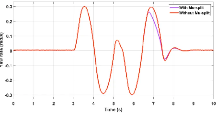
For a second maneuver, let us imagine that one side of the road gets wet. This is a frequent situation called the µ-split. We keep the same input of the driver as in the normal situation to see if the driver should have change its inputs. Results are shown in Figure 9.

Figure 9. The vehicle’s yaw rate in case of an open-loop control – double lane change maneuver with/without µ-split.

As Figure 9 shows, the vehicle starts losing its effectiveness when a µ-split occurs. Drivers have to adapt their inputs when an external disturbance appears. A closed-loop is definitely essential in case of autonomous driving.

To summarize, the concept of robustness is not defined when it comes to open-loop control. The human driver is therefore essential to face any external disturbance.

Ongoing Work on Closed Loop Strategies

As we have mentioned, open-loop strategies are accepted today since the human driver is the high-level controller that closes the loop. Therefore, for an autonomous vehicle, closing the loop is mandatory. In the following, we will carry the same maneuver using the same Renault Talisman to show the benefit of a closed-loop strategy with respect to an open one.

Control Architecture

The control strategy depends now on the yaw rate error since we can feed back the real yaw rate of the vehicle. The same yaw rate target as in (7) can be adopted to be followed by the closed-loop strategy. The distribution strategy remains the same. The control architecture now becomes as depicted in Figure 10.

Figure 10. Closed-loop architecture for a 4WS vehicle with VDC. The autopilot commands can be generated by a Model Predictive Controller (MPC) as in [12]. In addition, the objective of closing the loop is to add robustness to the control strategy. The motivation is to be independent from a human driver. Therefore, robust high-level controllers should be synthesized. To do so, we use ℋ∞ control

synthesis.

Controllers Synthesis

Thanks to ℋ∞ synthesis, we can take into account parameters and

dynamics uncertainties explicitly [21]. Not only the external disturbances are dealt with thanks to a closed loop architecture, but also the control strategy is robust with respect to the vehicle and actuators’ modeling uncertainties. However, this does not include the tire-road friction change, or the severe longitudinal and cornering stiffness change when the tires are replaced by the driver using completely different tires. An adaptive control should be privileged over a robust control, since this latter can be too conservative. This though goes beyond the scope of this paper.

In the following, we present only the synthesis for the 4WS robust controller, but it should be known that the same methodology is adopted for the VDC controller. ℋ∞ synthesis is a Model Based

Design (MBD) technique. For the 4WS controller, we need then the transfer function from the rear steering angle to the yaw rate:

𝑇_𝛿_𝑟_→𝜓̇(𝑠) = 𝐾_𝛿 𝑟(𝑉𝑥) 1 − 𝑠 𝑍𝛿𝑟(𝑉𝑥) 𝑠2 𝜔𝑛2(𝑉𝑥) + 2 𝜁(𝑉𝑥) 𝜔𝑛(𝑉𝑥)𝑠 + 1 (21)

(8)

Page 7 of 10 Where:

 𝐾𝛿𝑟(𝑉𝑥) : is the rear steering angle steady-state gain,

 𝑍𝛿𝑟(𝑉𝑥) : is the rear steering angle zero,

 𝜔𝑛(𝑉𝑥) : is the natural frequency of the vehicle,

 𝜁(𝑉𝑥) : is the damping ratio of the vehicle.

Next, the control specifications should be expressed in a ℋ∞ norm

that can be defined for a plan 𝐺 as:

‖𝐺‖_∞= sup𝜔≥0|𝐺(𝑗𝜔)|

(22) To do so, 𝑇_𝛿

𝑟→𝜓̇(𝑠) is augmented by weighting functions that specify

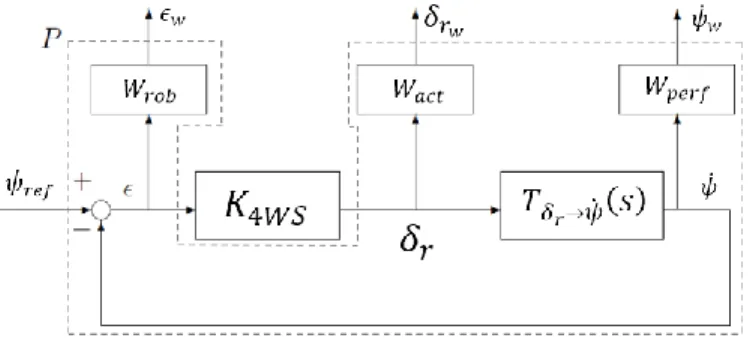
the desired control objectives [21]. Three objectives are selected: yaw rate tracking, commands moderation to respect the actuators and vehicle’s limits, and tracking robustness. Figure 11 describes this control problem.

Figure 11. Triple-criteria ℋ∞ problem for 4WS control synthesis.

The signals with the subscript “𝑤” are the weighted signals. 𝑊𝑝𝑒𝑟𝑓 is

the tracking performance weighting function, 𝑊𝑎𝑐𝑡 is the commands

moderation weighting function and 𝑊𝑟𝑜𝑏 is the tracking robustness

weighting function. To solve this problem, we use simply Matlab Robust Control Toolbox®_{. Moreover, as the transfer function depends}

on the vehicle’s speed, gain-scheduling is adopted to adapt the control strategy. The value of the speed is fed to the different robust controllers also. Additional details can be found in [2].

Co-Simulations Results

The same co-simulation methodology is adopted here again. Since we want to prove the robustness of the control strategy, we start with the double lane change with the µ-split. Results are shown in Figure 12.

Figure 12. The vehicle’s yaw rate in case of a closed-loop control – double lane change maneuver with µ-split.

As Figure 12 shows, in the second lane, as soon as the vehicle starts losing its effectiveness, the yaw rate error is amplified, the controller generates higher commands, and the vehicle recover its nominal behavior to follow the yaw rate target.

Now let us imagine a more severe maneuver with higher speed, for example 130 km/h in a highway, and higher steering input. Results are shown in Figure 13.

Figure 13. The vehicle’s yaw rate in case of a closed-loop control – severe double lane change maneuver with µ-split.

Since the 4WS system has not been saturated, the VDC remained deactivated. A clear loss of stability is observed at the end of the maneuver. We think that with a better coordination when activating both systems can solve this problem.

In other words, the robustness problem can be solved simply by closing the loop. However, using one system at a time, can be too conservative which limits the real potential of the car. Simultaneous operation of systems should privileged to face more severe situations.

Need for Optimal Control Allocation Strategies

The human driver does not only manage the disturbance rejection, but also the coordination of maneuvers. In case of autonomous vehicles, prioritization solutions will not be sufficient. Optimal Control Allocation (CA) strategies should be adopted [5]. In this case, we need a high-level controller that specifies the motion of the vehicle independently from the systems implemented, then a control allocation strategy to distribute optimally the control request. The control architecture should be transformed into the one described in Figure 14.

Figure 14. Closed-loop architecture with Optimal Control Allocation strategy for a 4WS vehicle with VDC.

Here, both 4WS and VDC systems can be activated in order to expand the vehicle’s potential. However, the tires could be solicited

(9)

Page 8 of 10

both longitudinally and laterally. Due to the friction ellipse concept [13], longitudinal tire forces and lateral tire forces are coupled. This should be taken into account before distributing any request. This is why the control allocation is done at the mid-level, between the vehicle physical variables and the actuator commands, namely, at the tire level. A simple, yet a combined tire model should be used. We use the linear tire model with varying parameters developed in [22]. Regarding the high-level and low-level controllers, ℋ∞ synthesis is

adopted. In the following, only the control allocation is described since it is the main added value of this control strategy.

Control Allocation Algorithm

The high-level controller computes a total yaw moment 𝑀𝑧𝑡𝑜𝑡 to be

distributed. The optimal distribution problem, in case of the 4WS and the VDC systems, can be formulated as follows: Find the control

vector 𝑢⃗ = [𝐹𝑥𝑓𝑙 𝐹𝑥𝑓𝑟 𝐹𝑥𝑟𝑙 𝐹𝑥𝑟𝑟 𝐹𝑦𝑟_𝑐]𝑡 such that:

[−𝑡 2 𝑡 2 −𝑡 2 𝑡 2 −𝑙𝑟] 𝑢⃗ = 𝑀𝑧𝑡𝑜𝑡 (23) Subject to − [ √(𝜇𝑓𝑙𝐹𝑧𝑓𝑙) 2 − 𝐹_𝑦2_𝑓𝑙 √(𝜇_𝑓𝑟𝐹𝑧𝑓𝑟) 2 − 𝐹𝑦𝑓𝑟 2 √(𝜇𝑟𝑙𝐹𝑧𝑟𝑙) 2 − 𝐹𝑦𝑟𝑙 2 √(𝜇_𝑟𝑟𝐹𝑧𝑟𝑟) 2 − 𝐹𝑦𝑟𝑟 2 √(𝜇𝑟𝐹𝑧𝑟) 2 − 𝐹𝑥𝑟 2 ] ≤ [ 𝐹𝑥𝑓𝑙 𝐹𝑥𝑓𝑟 𝐹𝑥𝑟𝑙 𝐹𝑥𝑟𝑟 𝐹𝑦𝑟] ≤ [ √(𝜇𝑓𝑙𝐹𝑧𝑓𝑙) 2 − 𝐹_𝑦2_𝑓𝑙 √(𝜇_𝑓𝑟𝐹𝑧𝑓𝑟) 2 − 𝐹𝑦𝑓𝑟 2 √(𝜇𝑟𝑙𝐹𝑧𝑟𝑙) 2 − 𝐹𝑦𝑟𝑙 2 √(𝜇_𝑟𝑟𝐹𝑧𝑟𝑟) 2 − 𝐹𝑦𝑟𝑟 2 √(𝜇𝑟𝐹𝑧𝑟) 2 − 𝐹𝑥𝑟 2 ] (24) With the superscript 𝑡 means the transpose, and 𝐹𝑧𝑖𝑗 is the vertical

load at the tire (𝑖𝑗). This CA problem is solved online at each sampling time step. Various algorithms have been tested in [13] and [14]. The Weighted Least Squares (WLS) formulation using a one stage Active Set Algorithm (ASA) to solve the problem has proven its efficiency and relative rapidity with respect to the other methods. The optimal solution can be formulated as follows:

𝑢 ⃗ 𝑜𝑝𝑡= 𝑎𝑟𝑔 {min𝑢⃗⃗ 𝑚𝑖𝑛≤𝑢⃗⃗ ≤𝑢⃗⃗ 𝑚𝑎𝑥(∑ 𝛾𝑖‖𝑾𝒊(𝑩𝒊𝑢⃗ − 𝑣 𝑖)‖ 2 𝑙 )} (25) Where:

 𝑙 : is the number of objectives,  𝛾𝑖 : is the weight of the 𝑖𝑡ℎ objective,

 𝑾𝒊 : is the non-singular weighting matrix of the 𝑖𝑡ℎ objective,

 𝑩𝒊 : is the effectiveness matrix relating the control vector to

the desired 𝑖𝑡ℎ_objective,

 𝑣 𝑖 : is the desired vector of the 𝑖𝑡ℎ objective,

Multiple objectives can be taken into account depending on the car manufacturer desire. Once all the objectives formulated, the problem should be reformulated as an ASA one as follows:

𝑢⃗ 𝑜𝑝𝑡= 𝑎𝑟𝑔{min𝑢⃗⃗ 𝑚𝑖𝑛≤𝑢⃗⃗ ≤𝑢⃗⃗ 𝑚𝑎𝑥(‖𝑨𝑢⃗ − 𝑏‖)}

(26) The ASA solver can be then directly applied.

Co-Simulations Results

The remaining problem that we have observed in the closed-loop strategy is the loss of effectiveness in case of severe double lane change, since only one system is activated at a time. We redo the same maneuver with an optimal CA strategy. Figure 15 shows the results.

Figure 15. The vehicle’s yaw rate in case of a closed-loop control with CA – severe double lane change maneuver with µ-split.

In contrast of the classic closed-loop without optimal coordination, the vehicle remained stable even at the second lane. This mainly due to the fact that both systems have activated without any conflicts as Figure 16 shows.

Figure 16. The 4WS and VDC systems commands in case of a closed-loop control with CA – severe double lane change maneuver with µ-split. The left brakes have been activated in the first change of lanes. But higher brake commands have been requested at the second lane with the µ-split. This gave the vehicle the supplementary yaw moment needed to stabilize the vehicle. When several systems are activated, the potential of an autonomous vehicle can be expanded to cope with more severe situations.

(10)

Page 9 of 10

Future Work: Model Predictive Control

Allocation Strategies

In the previous results, communication delays were neglected. Through our experimentations, we found out that the 4WS system presents a delay of 50ms while the VDC presents a delay of 180ms. This adds an additional challenge to the distribution problem. In particular, if the 4WS system is saturated, the VDC system cannot instantly takeover the maneuver due to the communication delays. Two different solutions are being tested in the industry: the adoption of Ethernet cables to accelerate the communication response, or a Model Predictive Control Allocation (MPCA) to distribute the commands while taking into account the communication delays. The first solution goes beyond the scope of our research. In the following, we will discuss only the MPCA solution.

The MPCA technique is inspired ,as its name reveals, from the MPC. The MPC is an online optimization-based control technique that aims to solve a finite-horizon optimization problem at each sampling time. An internal discretized dynamic model is used to predict the behavior of the system, and the optimizer generates the required control inputs in order to satisfy the desired performances along a chosen prediction horizon. The MPC objective cost function is usually taken as follows [23]:

𝐽(𝑘) = ∑ 𝑄(𝑖)(𝑥̂(𝑘 + 𝑖|𝑘) − 𝑟(𝑘 + 𝑖|𝑘))2+ 𝑅(𝑖)(𝑢̂(𝑘 + 𝑖|𝑘))2

𝑇

𝑖=1

(27) Where 𝑘 is the current time step, 𝑥̂ is the estimated state, 𝑟 is the reference trajectory, 𝑢̂ is the optimal control sequence, and 𝑇 is the prediction horizon length. The first term in 𝐽(𝑘) represents the reference tracking performance, and the second one represents the control effort mitigation. The weights 𝑄(𝑖) and 𝑅(𝑖) enable favoring one objective over another. In addition, as far as an optimization problem is concerned, the MPC is capable of handling constraints at both the control input level and the state level.

For the MPCA, the same idea can be adapted to the optimal distribution problem. In this case, the cost function becomes [24]:

𝐽(𝑘) = ∑ (∑ 𝐵𝑗𝑢𝑗(𝑘 + 𝑖) − 𝑣(𝑘 + 𝑖) 5 𝑗=1 ) 2 + 𝛾𝑊𝑢(𝑗) (𝛿𝑗(𝑘 + 𝑖)) 2 𝑇 𝑖=1 (28) With here 𝛿𝑗 corresponds to the actuators commands. The mid-level

and low-level layers of the Figure 14 are now merged, since the allocation strategy takes into account both the tire couplings and actuators real dynamics with the communication delays. The prediction horizon in this case should be at least superior to the bigger time-delay. For example, we have identified a time-delay of almost 180ms regarding the VDC system. 𝑇 should be then at least equal to 200ms. For a sampling time of 10ms, this means that we have to solve 20 optimization problem at each time step. More efficient Electronic Control Units (ECU) would be required. Currently, we first focus our efforts in validating the classic control allocation in real-time. The communication delays are approximated by Padé approximations and taken into account in rather the

high-level controller. This controller becomes too conservative in this case. The performance of the overall strategy is then penalized. The MPCA, which is expected to improve the overall vehicle motion strategy, constitutes our future work.

Co-Simulations Results

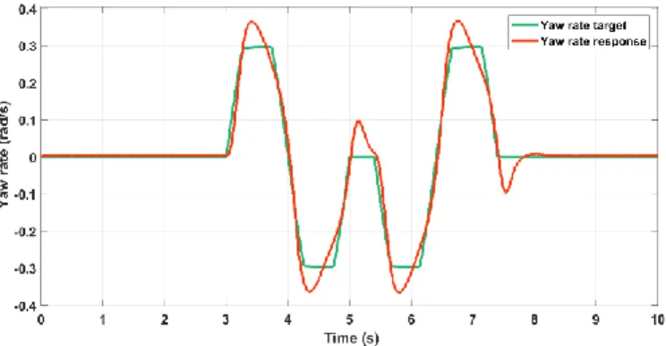
In this case, we take into account the global time-delay of the different systems. We first apply the classic CA method, and then the MPCA. Fig. 17 shows the results.

Figure 17. Comparison of the classic CA and the MPCA in case of severe yaw rate request ([24]).

The MPCA makes the vehicle more reactive since it takes into account the time-delays of each system. In this way, when the saturation of one of the systems is predicted, the secondary system can be activated few steps before the effective saturation of the primary system.

Conclusions

In this paper, a roadmap for global chassis control has been presented. An example of a real passenger car is presented in case of open loop control. Since more robustness is expected from

autonomous vehicles, the closed loop strategy has been presented for the same example. Finally, an optimal control allocation strategy has been introduced to solve the coordination problem. The results prove the need of closing the loop especially when no human driver monitors the vehicle, and also the necessity of optimal control allocation when both systems should be simultaneously operated. This gives a clear roadmap on how global vehicle motion control strategies should evolve.

This paper lacks however some experimental results to validate our claims. The different strategies are actually being tested in different prototypes. Future research papers will focus on the experimental comparison of the different strategies along with the development of the MPCA strategy.

References

1. Nadkarni, I.T., "Parliament approves EU rules requiring life-saving technologies in vehicles," European Parliament Press

Releases. April 2019.

2. Kissai, M., Monsuez, B., Martinez, M., and Tapus, A., "Optimal Coordination of Chassis Systems in Simultaneous Operations,"

(11)

Page 10 of 10

SAE Int. J. of Connected and Automated Vehicles. Special Issue

on Revisiting Chassis and Powertrain Design for Automated Vehicles, 2019, JCAV-2019-0018, Accepted on August 2019. 3. Singh, A., Kumar, A., Chaudhary, R. and Singh, R., "Study of 4

Wheel Steering Systems to Reduce Turning Radius and Increase Stability," International Conference of Advance Research and Innovation, 2014.

4. Kissai, M., Monsuez, B., Tapus, A. and Martinez, D., "Control Allocation of Active Rear Steering and Vehicle Dynamics Control Using a New Tire Model," Int. J. Mech. Eng. Robot. Res., 7(6):608-616, 2018. doi: 10.18178/ijmerr.7.6.608-616. 5. Selby, M.A., "Intelligent Vehicle Motion Control," University of

Leeds, 2003.

6. Kissai, M., Monsuez, B. and Tapus, A., "Review of integrated vehicle dynamics control architectures," 2017 European Conference on Mobile Robots (ECMR), 2017, pp. 1-8, doi: 10.1109/ECMR.2017.8098687.

7. Besselink, I., Veldhuizen, T. and Nijmeijer, H., "Improving yaw dynamics by feedforward rear wheel steering," 2008 IEEE Intelligent Vehicles Symposium, 2008, pp. 246-250. doi: 10.1109/IVS.2008.4621314.

8. Allwright, J., "Four Wheel Steering (4WS) on a Formula Student Racing Car," SAE-A Vehicle Technology Engineer –

Journal, 1, 2015. doi: 10.7790/vte-j.v1i1.5.

9. Kissai, M., Monsuez, B., Tapus, A., Mouton, X. and Martinez, D., "Gain-Scheduled H∞ for Vehicle High-Level Motion Control," Proceedings of the 6th_{International Conference on}

Control, Mechatronics and Automation, 2018, pp. 97-104, doi: 101145/3284516.3284544.

10. Ivanov, V. and Savitski, D., "Systematization of Integrated Motion Control of Ground Vehicles," IEEE Access 3:2080- 2099, 2015, doi:10.1109/ACCESS.2015.2496108.

11. Kissai, M., Monsuez, B., Mouton, X., Martinez, D. and Tapus, A., "Adaptive Robust Vehicle Motion Control for Future Over-Actuated Vehicles," Machines, 7(2), 26, 2019. doi:

10.3390/machines7020026.

12. Kissai, M., Mouton, X., Monsuez, B., Martinez, D. and Tapus, A.,"Optimizing Vehicle Motion Control for Generating Multiple Sensations," 2018 IEEE Intelligent Vehicles Symposium (IV), 2018, pp. 928-935, doi: 10.1109/IVS.2018.8500563.

13. M. Kissai, X. Mouton, B. Monsuez, D. Martinez and A. Tapus, "Complementary Chassis Systems for Ground Vehicles Safety," 2018 IEEE Conference on Control Technology and Applications (CCTA), 2018, pp. 179-186, doi: 10.1109/CCTA.2018.8511622. 14. Bodson, M., "Evaluation of Optimization Methods for Control

Allocation," Journal of Guidance, Control, and Dynamics 25(4): 703-711, 2002, doi: 10.2514/2.4937.

15. Pacejka, H.B., "Tire and Vehicle Dynamics," SAE International and Butterworth Heinemann, 2012.

16. Soltani, A.M., "Low Cost Integration of Electric Power-Assisted Steering (EPAS) with Enhanced Stability Program (ESP)," Cranfield University, 2014.

17. Sehyun, C. and Gordon, T.J., "Model-based predictive control of vehicle dynamics," International Journal of Vehicle

Autonomous Systems 5(1-2): 3-27, 2007, doi:

10.1504/IJVAS.2007.014945.

18. Milliken, W.F. and Milliken, D.L., "Race Car Vehicle Dynamics," SAE International, Premiere Series, 1995, isbn: 9781560915263.

19. Vilela, D. and Barbosa, R., "Analytical Models Correlation for Vehicle Dynamic Handling Properties," Journal of the Brazilian

Society of Mechanical Sciences and Engineering, 33, 437-444,

2011, doi: 10.1590/S1678-58782011000400007.

20. Kissai, M., "Optimal Coordination of Chassis Systems for Vehicle Motion Control," ENSTA Paris, 2019.

21. Scorletti, G. and Fromion, V., "Automatique Fréquentielle Avancée," Ecole Centrale de Lyon, 2009.

22. Kissai, M., Monsuez, B., Tapus, A. and Martinez, D., "A new linear tire model with varying parameters," 2017 2nd IEEE International Conference on Intelligent Transportation Engineering (ICITE), Singapore, 2017, pp. 108-115, doi: 10.1109/ICITE.2017.8056891.

23. Hanger, M.B., "Model Predictive Control Allocation", Master thesis, Institutt for teknisk kybernetikk, Norwegian University of Science and Technology, 2011.

24. Kissai, M., Monsuez, B., Mouton, X., Martinez, D. and Tapus, A., "Model Predictive Control Allocation of Systems with Different Dynamics," 2019 IEEE Intelligent Transportation Systems Conference (ITSC), 2019, pp. 4170-4177, doi: 10.1109/ITSC.2019.8917438.