Experiments and Models of Active and Thermal Imaging Under Bad Weather Conditions

Any correspondence concerning this service should be sent to the repository

administrator:

[email protected]

O

pen

A

rchive

T

oulouse

A

rchive

O

uverte (

OATAO

)

OATAO is an open access repository that collects the work of Toulouse researchers and

makes it freely available over the web where possible.

This is an author-deposited version published in:

http://oatao.univ-toulouse.fr/

Eprints ID: 11730

To cite this version:

Bernard, Erwan and Rivière, Nicolas and Renaudat, Mathieu and

Guiset, Pierrick and Péalat, Michel and Zenou, Emmanuel Experiments and Models of

Active and Thermal Imaging Under Bad Weather Conditions. (2013) In: SPIE Defence

+ Security, 23 September 2013 - 26 September 2013 (Dresden, Germany).

Experiments and models of active and thermal imaging under bad

weather conditions

Erwan Bernard*

, Nicolas Riviere

, Mathieu Renaudat

, Pierrick Guiset

, Michel Pealat

,

Emmanuel Zenou

a

Sagem, 100 avenue de Paris 91300 Massy, France

b

ONERA, The French Aerospace Lab, 31055 Toulouse, France

c

ISAE DMIA, 10 Avenue Edouard Belin 31000 Toulouse, France

ABSTRACT

Thermal imaging cameras are widely used in military contexts for their night vision capabilities and their observation range; there are based on passive infrared sensors (e.g. MWIR or LWIR range). Under bad weather conditions or when the target is partially hidden (e.g. foliage, military camouflage) they are more and more complemented by active imaging systems, a key technology to perform target identification at long range. The 2D flash imaging technique is based on a high powered pulsed laser source that illuminates the entire scene and a fast gated camera as the imaging system. Both technologies are well experienced under clear meteorological conditions; models including atmospheric effects such as turbulence are able to predict accurately their performances. However, under bad weather conditions such as rain, haze or snow, these models are not relevant. This paper introduces new models to predict performances under bad weather conditions for both active and infrared imaging systems. We point out their effects on controlled physical parameters (extinction, transmission, spatial resolution, thermal background, speckle, turbulence). Then we develop physical models to describe their intrinsic characteristics and their impact on the imaging system performances. Finally, we approximate these models to have a “first order” model easy to deploy for industrial applications. This theoretical work will be validated on real active and infrared data.

Keywords: Active imaging, thermal imaging, adverse condition, rainfall, MILPAT, rainfall modeling

1. GENERAL CONTEXT

Thermal and active imageries are two complementary technologies which can be used for both day and night visions.

An active imaging system involves a light source to illuminate the object to be observed and a camera to collect the

reflected light. In most active imaging systems, the light source is a short-pulsed and directional laser and the camera is a gated one. When the camera and the laser pulse are both synchronized, one can image objects at a selected distance from the system. The light backscattered by the surrounding is eliminated from the final image and 3D or pseudo-3D imagery becomes possible. This technique is independent from natural illumination (e.g. sunlight) and can be used by day and night. Active imaging usually works in the near infrared (NIR) and short wave infrared (SWIR) wavelength ranges but SWIR is preferred for eyes safety issues. In this spectrum range, target characteristics are determined by their reflective properties.

A thermal imaging system involves an infrared (IR) camera to detect radiation from emissive targets in the IR range.

Thermal imaging does not need any external light source or gated camera to be operated but some sensors need to be cooled at low temperature. Thermal imaging works in mid-wave infrared (MWIR) and long-wave infrared (LWIR) spectral ranges. In these spectral ranges, the target characteristics are determined by their emissivity and temperature. Day and night visions are possible without external light source.

Active imaging systems use shorter wavelength than thermal imaging and achieve a better spatial resolution (the diffraction limit is reduced). Well-designed long range systems are limited by atmospheric turbulence effects which blur the images and impact the illumination homogeneity.

Active and thermal imaging techniques have different behaviours and bring together different characteristics such as temperatures or reflectance. While thermal imaging performances have been characterized by 30 years of experiments, active imaging needs to be evaluated in many scenarios especially under bad meteorological conditions (e.g. rain or haze).

In order to demonstrate the active imaging capabilities in surveillance applications, The French MoD (DGA) funded a prototype system named MILPAT for “Laser Imaging Module for Terrestrial Applications”. It allows the comparison between active and thermal imaging. Figure 1 presents a general view of the instrument and two typical images obtained during the trial campaign. Sagem and Thales collaborated to include (i) an active system, (ii) a Sagem high performance thermal camera (MATIS LR) and, (iii) a laser rangefinder mounted on a turret for tracking and sight positioning.

Figure 1 MILPAT prototype systems assembled during trial campaign in 2013. Two images of the Bourges cathedral (France) taken with MILPAT in active and thermal.

Since December 2011, MILPAT has been providing active and thermal images in field conditions during several trial campaigns for which meteorological conditions were simultaneously monitored: turbulence (Cn² is determined using scintillometers), rain rate and visibility. A data base was created with various objects and meteorological conditions. Experimental description of assumed degradation can be observed, especially for thermal imaging which is strongly influenced by weather conditions. We consider thermal images extracted from our last trial campaign under clear sky and rainy conditions (see fig. 2). If during day time the sunlight heats the observed objects of the scene as the cathedral roof (black in the visible spectral range) the images present on fig. 2 a huge contrast which decreases or even vanishes after the night or a cloudy day. We observe under rainy conditions a decrease of the image contrast as shown on fig. 2b. This is due to the reduction of the solar illumination and the cooling of object surfaces by water. This phenomenon can also be linked to the path radiance and atmospheric transmission.

Figure 2. Thermal images with different atmospheric conditions (during day time). Clear sky condition on the left image and on the right under a light rain.

Active imaging benefits from the short gate duration of the sensor yielding a very low stray light. In this configuration, active sensors show the same characteristics in day and night cases. In rainy days, we observe a decrease of the contrast and an increase of the spatial resolution. This is due to the reduction of the turbulence level under rainfall (fig. 3b).

(a)

(b)

Active imaging Thermal imaging

Figure 3. Active images with two different atmospheric conditions; left image: in clear sky condition; right image: under a light rain.

To go deeper in the involved physical phenomena we need to develop a predictive model including atmospheric turbulence and rainfall effects. The next section presents rainfall model. Then we will present images of a trial campaign realized with MILPAT instrument. The rainfall impact on images will be discussed.

2. ISAAC CODE

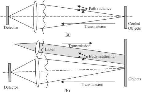
We illustrate by different ways in fig. 4 how rainfall can deteriorate the image quality for both thermal and active imaging. As previously seen, the reduction of the transmission is a typical effect but not the major one. This is especially true for active imaging since transmission decrease could be compensated by an increase of the laser power. On the one hand, the surrounding can impact thermal and active imaging techniques: e.g. the backward transmission and the wave front distortion are disturbed by the raindrops located between the sensors and the object. On the other hand, we identify effects mainly depending on the imaging technique. For thermal imaging, droplets emit radiations in the thermal spectrum range in relation with their emissivity and their temperature. The variation of the temperature on a scene can also be washed out by the rainfall. As a consequence, the contrast of the image is reduced. Active imaging could be disturbed by backscattered light but this effect can be neglected as we use a gated camera. However, active imaging is also disturbed on illumination path. We need an accurate model to characterize the image deterioration under rain conditions. This model should consider all the effects summarized on fig. 4.

Figure 4. Environment contribution on images degradations for active and thermal imaging.

(a)

(b)

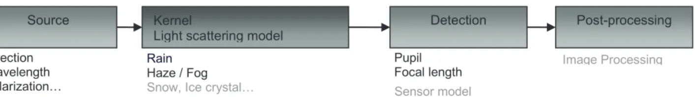
To compute angular information of the rainfall impacts, we developed ISSAC code. This model considers the entire acquisition chain (see fig. 5) from the light source to the sensor. The simulation kernel is based on a Monte-Carlo method and evaluates the light propagation through a scattering medium.

This modular code allows fast upgrades and modifications. Physical models can be added or changed easily. For example, the interaction between light and particles can be switched between optical geometry and a pre-calculated phase function. Many parameters can be changed in ISAAC code depending on the selected scenario (from the system specifications, like wavelength, pupil…, to the scene, like geometry, kind of phenomenon…). Fig 5 depicts the general architecture of our ISAAC code.

Figure 5. Architecture scheme of Isaac code

Light propagation is modeled through rainfall from rain-drop characteristics: size distribution, phase function, shape and water refractive index. ISAAC code is based on physical models found in literature. In next sections, a description of each model used in ISAAC code is described.

2.1 Drop size distribution

The drop size distribution defines the distribution and the number of drops in a volume. Considering simplified laws, this function depends on the rain rate expressed in mm.h-1: e.g. we talk about light or heavy rain respectively for rain rates equal to 5 mm.h-1 or 25 mm.h-1. We note that these values are averaged in large areas and higher rain rates values can be locally observed.

A large number of distributions can be found in the literature. One can find typical distributions given by D. Atlas [8]. Hereafter, we only consider distributions applicable to our application and corresponding to the identified wavelength range. Drop size distributions are parameterized functions where constants are adjusted according to experimental data. Thus each application considers different parameterization depending on scenarios.

2.1.1 Marshall-Palmer distribution

A well known study was published by Marshall and Palmer in 1948 [5]. This distribution characterizes the rain in mid-latitude and is described by a simple exponential law [7].

( )

D

(

u

D

)

N

=

8

.

0

´

10

exp

-

4

.

10

where NMP is the Marshall-Palmer drop size distribution density (m-4). In this formula the rain rate u is expressed in r

mm.h-1 and D is the raindrop diameter (see fig. 6).

The distribution coefficients (front coefficient and exponential decay) are fully found by a single radar measurement. This model has a major drawback: as it has been developed for radar purposes, large rain drop diameters should be considered.

2.2 Laws-Parsons distributions

Another formula of the distribution was published by Laws and Parson in 1943 [2][6] for applications in the optical wavelength range. This drop size distribution is described by a gamma law. It is related to a more realistic intensity for smaller particles (fig. 6). The law coefficients are quite complex to be measured. We need a more complete measurement method (optical or mechanical) and not only a simple radar approach. A comparison of these both distributions is shown on fig. 6. The difference for small particles is visible.

Detection Source Kernel

Light scattering model

Post-processing Direction Wavelength Polarization… Rain Haze / Fog

Snow, Ice crystal…

Pupil Focal length

Sensor model

(

D

)

u

D

(

u

D

)

N

=

1

.

98

´

10

exp

-

5

.

38

raindrop diameter.

Figure 6. Drop size distribution density [m-4] versus D [mm] at three rain rates. Solid lines are Marshall-Palmer curves and dashed lines are Laws-Parsons Curves. The rain rates are set to 2 mm.h-1 for light rain and 50 mm.h-1 for extreme rain.

2.3 Phase function

The phase function allows easier representation of the interaction between light and a single particle. It depends on the water absorption, the refractive index, the size and the shape of a droplet. This function defines the angular distribution of the light after its interaction with one raindrop. Phase function can be analytically estimated according to the Mie theory developed for spherical particles or directly computed with an electromagnetic code. Such a function can be computed for each size of the droplets. Our ISAAC code considers a limited number of diameters to reduce input data and to interpolate the function for missing drop diameters.

2.3.1 Raindrop shape

The shape of the droplet depends on various parameters such as the altitude or the wind speed. The change of the droplet geometry has low impacts on macroscopic characteristics. As a consequence we only consider spherical raindrops. To enhance polarization effects, a more realistic model was published by Chuang and Beard [4]. This model uses a spherical shape for particles (diameter under 0.5 mm). Particles are deformed by the following equation for larger raindrops. In this model the shape deformation depends on the size of the particle.

Chuang and Beard give the deformation which the followed expression at the 10th order:

mm

a

n

c

a

r

cos(

)

,

0

.

5

1

)

(

>

ú

û

ù

ê

ë

é

+

=

å

q

q

where

r

(

q

)

q

a

n

Figure 7. Raindrop shapes for particles between 2 mm and 6 mm [9].

ISAAC code does not directly implement the raindrop shape developed by Chuang and al.Nevertheless we approximate this shape of such particles by an ellipsoid. This consideration allows polarization computation as the shape modification is more realistic than the one modeled with spherical particles.

2.3.2 Water refractive index

The complex refractive index can be represented by the real part of the refractive index (fig. 8a) and by the extinction (linked to the imaginary part fig. 8b). The extinction of the signal corresponds to the absorption within the medium. The complex refractive index mainly depends on the wavelengths. We observe a strong variation of the real and imaginary part of the refractive index according to the spectrum range (Visible, SWIR, Thermal/MWIR) as shown on fig. 8.

Figure 8. Water refractive index and extinction for several technologies (SWIR: active imaging, MWIR: thermal imaging).

Between SWIR (for active imaging) and MWIR (for thermal imaging) bands, we note a strong difference concerning the water absorption coefficient. There are 2 orders of magnitude in water absorption between these two wavelength ranges. This coefficient describes the interaction of the light within a uniform medium but it doesn’t take into account the scattering attenuation by the droplet/atmosphere interfaces. Even if this short analysis would tend to prove that absorption is dominant (especially in the thermal range), the work presented in the next section will change this perspective.

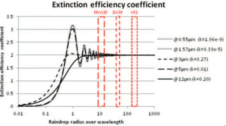
2.3.3 Extinction efficiency factor

Most particles have an obvious geometrical cross section. The dimensionless constants called the efficiency factors are defined as the ratio of the extinction cross section over the geometrical cross section [1]. A complete computation of the extinction efficiency factor using the Mie theory considers the spherical shape and the refractive index of the droplets. The efficiency factor (fig. 9) is used to calculate the phase function and describes the energy losses by the light scattered by a single raindrop. Light scattering effects are related to the refraction and the reflection of the light in the raindrop and to the diffraction by a particle.

.

Figure 9. Extinction efficiency coefficient in function of ration between raindrop radius and wavelength.

We identify several scenarios for MWIR thermal imaging and SWIR active imaging. Adverse conditions include different rain rates. The size of the droplets under rainfall is considered upper than 50 µm, thus for all wavelengths shorter than 5 µm, the efficiency factor is equal to 2 and does not depend on the wavelength value. Van de Hulst [1] explained this value of the efficiency factor using the extinction paradoxes. The optical properties of the droplet (e.g. absorption) don’t have any impact on the global transmission through the rainfall at the fixed wavelength. This interpretation is used in the next section to estimate a value of the modulation transfer function (MTF). A partial validation of our ISAAC code is also presented in section 2.4.

2.4 Partial validation on the modeled transmission

ISAAC code uses a numerical method based on a Monte-Carlos approach and empirical models like the drop-size-distribution. Although physical laws are considered, our code needs to be validated on experimental measurements and other existing models. The analytical model described in the following part is implemented in Modtran [10]. We consider Modtran to validation our code for transmission aspects. On the one hand, we simulate the transmission through rainfall with ISAAC code. On the other hand, we use the Modtran-like model based on the Marshall-Palmer distribution and an analytical expression of the extinction efficiency coefficient for small spherical particles.

2.4.1 Analytical transmission model

Rainfall implies large kind of optical degradations. The transmission is selected from other macroscopic parameters as it is easy to be measured and analytically defined. The impact of the rainfall on the transmission constitutes a first step of our study. The light propagation through the scattering medium and the degradation on active and thermal imaging will be evaluated.

The transmission is calculated by the following expression:

d Bext

e

T

=

This expression is a common exponential law where T is the transmission through a distance d. The scattering medium is characterized by its extinction coefficient B expressed in mext -1.

() (

)

ò

=

8

,

,

n

D

dD

D

Q

D

N

B

l

p

The extinction coefficient depends on raindrop diameter D and on the size distribution N

( )

2.4.2 Comparison

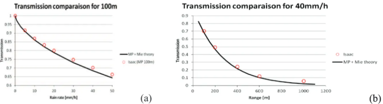
The comparison between the analytical model and our ISAAC code is achieved by considering the transmission with a variation of several parameters. On fig. 10, we plot the transmission at a fixed range versus different rain rates (see fig. 10a) and different ranges for a fixed rain rate (fig. 10b).

Differences can be found in relation with the diffraction and the estimation of the extinction efficiency section. ISAAC code uses the geometrical optic approximation to model the light scattered by particles whereas the analytical model considers the entire Mie theory and therefore diffraction effects. In this work, we assume that this approximation is acceptable (low errors between results) because we introduce large rain droplets and multiple scattering can be neglected. Most of the photons are deflected out of the line of sight. This difference causes a small error of 2% on the transmission estimation.

Figure 10. Comparison between ISAAC code and an analytical model using Marshall-Palmer distribution and the Mie theory. (a): the propagation through 100 m long rain tunnel is considered. (b): a rain rate of 40 mm.h-1 is used..

2.5 Rain properties evaluation

Once our ISAAC code is validated, we can use it to estimate other interesting parameters such as the angular scattering. Fig. 11 represents the simple environment modelled: a monochromatic laser (no divergence) passes through a volume of the rainfall and the signal is collected on a spherical detector. We obtain the spatial information of the scattered light. Two results of this simulation are shown hereafter.

Figure 11. Representation of the spatial configuration. This environment is used by the two following simulations.

(b)

(a)

(b)

2.5.1 Order of magnitude of some rainfall characteristics

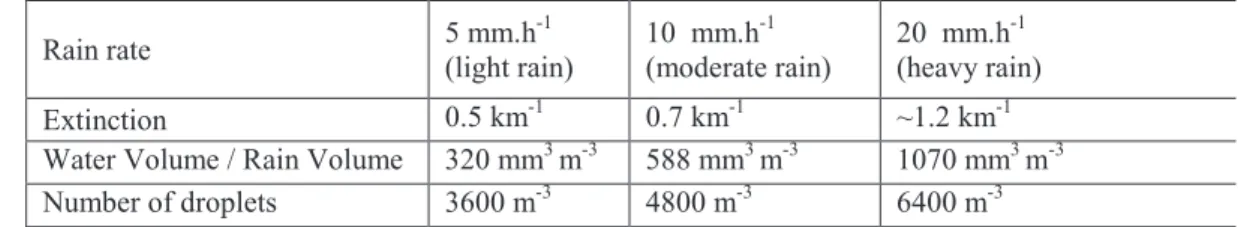
Basic statistics can be evaluated from simple simplifications of the initial model. Characteristics are summarized in the following table. These values give ideas about rainfall.

Rain rate 5 mm.h -1 (light rain) 10 mm.h-1 (moderate rain) 20 mm.h-1 (heavy rain) Extinction 0.5 km-1 0.7 km-1 ~1.2 km-1 Water Volume / Rain Volume 320 mm3 m-3 588 mm3 m-3 1070 mm3 m-3 Number of droplets 3600 m-3 4800 m-3 6400 m-3

Table 1. Various rainfall statistics for different input parameters. Marshall-Palmer distribution is considered.

2.5.2 Number of scattering events

ISAAC code allows multiple scattering to occur in the computation. First, we extract the number of scattering events. Fig. 12 shows results for two different ranges: 500 m and 1 km. These curves represent the histogram for 1 million photons in order to reach limit behaviour. We show on this figure that for a rain rate of 10 mm.h-1, a half number of photons is statistically scattered before 500 m. Moreover, the probability to have only one scattering event is evaluated to 35%. The percentage of photons with no-interaction and the light transmission are correlated: each photon interacting with a droplet is mainly scattered in a way different from the forward direction. As a consequence, photons collected by the sensor in the forward direction have no-interaction with the droplets. The same conclusion is obtained with the efficiency factor; the chemical composition of a particle has no effect on the light propagation at the fixed wavelength.

Figure 12. Number of interactions of a light beam. On the left the light passes through a 500 m long rain tunnel and through 1 km long on the right. This computation is realized with our Isaac code and 1millions of photons.

2.5.3 Angular scattering characteristics

In a second step, we determine the scattering characteristics of the rainfall. We consider the same geometry of the scene as the one defined in the previous section. Here, we simulate a 1 km-long rainfall. The light is angularly collected as this representation can be useful for imaging sensor. This approach allows determining halation phenomenon or evaluating MTF degradation by the rainfall. This parameter is also a macroscopic characteristic which can be easily measured during experimental validations. We note on fig. 13 a decrease of the scattered light versus the rain rate evolution and identify an offset correlated to the value of the rain rate. These observations are coherent as the evolution of the drop size distribution is insignificant from the rate evolution.

Figure 13. Scattering characteristics of light propagating through a 1km long rain tunnel.

2.6 Simplified model: Modulation Transfer Function model

The complete rainfall model is a crucial tool in developing new simple and empirical models. The modification of the atmospheric modulation transfer function (MTF) is of interest to describe the image degradation. This parameter is commonly used to characterize optical systems and should be evaluated under simple considerations.

In the previous section, the evaluation of the extinction factor puts the light on the independence between drop properties and drop cross sections. In section 2.5.1, we show that a large number of transmitted photons through the rainfall had no scattering event. In these conditions, raindrops can be considered as opaque spheres. Rain-shadows can be projected on the pupil (see fig. 14) and it allows determining an approximation of the MTF by computing an autocorrelation of the pupil.

Figure 14. Simple raindrop projection on the sensor pupil.

This approach corresponds to a really simple model as it considers a large approximation done for physicals phenomenon where considered scattering angles are very small. A first validation can be conducted comparing transmission results obtained with this new projection-model and the analytical-model already described in section 2.4.1.

Raindrops Detector

Raindrop projections Pupil

Figure 15. Simple raindrop projection on the sensor pupil for two values of the rain rate (10 mm.h-1 and 30 mm.h-1) and for a range of 1 km. On the right, comparison between the simplified MTF model and the analytical based on a Marshall-Palmer distribution and the Mie theory.

We assume in this new simplified MTF model that raindrops are fixed during an image acquisition. For active imaging applications, they can be considered as static particles for a short laser pulse duration. Nevertheless, the integration time in thermal imaging can reach (at most) 20 ms.

According to Gunn and Kinzer [13], raindrop terminal velocity is between 1 m.s-1 and 9 m.s-1 for a droplet diameter ranging from 200 µm to 5 mm. If we consider a mean particle size around 700 µm, its velocity is close to 3 m.s-1. These characteristics induce a fall of 6 cm during an integration time of 20ms. The raindrop velocity will induce also a change of the MTF. For a quick evaluation of the MTF degradation, simulations are achieved with a uniform velocity. We observe on fig. 16 a global decrease of each frequency within the rain rate. The horizontal component is also more impacted in function of the rain rate. Vertical perturbations are due to the fall of the raindrops and depend on the wind direction.

Figure 16. Simple raindrop projection on the sensor pupil for two different rain rates, for a range of 1 km and with an integration time of 20 ms. On the right, the MTF for different rain rates and orientations (horizontal and vertical) is presented.

2.7 Model accuracy

Modelled and experimental results are useful to determine the validity of our method and to identify the application field of our simplified model. Lots of experiments have been published to compare rainfall models and measurements [14]. The main issue of this characterisation is the non-spatial-uniformity of the rain (local measurements). For long range characterizations, local measured rain rate and local measured transmissions are strongly different from the reality. For instance Mattzler [14] presents different measurements from field test: in certain cases, he identified a factor 2 between experimental and modelled values of the extinction.

10 mm.h-1

5mm/h 20mm/h 30 mm.h-1

3. CONCLUSION

We developed a comprehensive model to study the propagation of the light through an adverse medium (rainfall). This code is based on a modular concept and allows futures evolutions. We can change the phase function, the particle size distribution and the shape of the scatterers. 3D objects with complex geometry can be introduced in the scene (targets with various optical properties on their facets). We plan to develop a complete validation scheme of our ISAAC code. The comparison between the analytical method and results obtained with our ISAAC code is an easy way to begin this. To achieve this complete and accurate validation we would compare our results with angular models and measurements of macroscopic parameters. Measurements are still in progress using rain-tunnels and cloud-chambers developed by ONERA. Meteorological conditions are fully controlled (rain rate, particle size distribution…).

The goal of this study is to model the modifications of images (active and thermal imaging) due to bad weather conditions. The propagation of the light through rainfall is a first step. The rainfall modifies the properties of a solid target such as the reflectance or the surface temperature. Future works would introduce these variations in ISAAC code. More simplified models with defined validity ranges will be developed to allow fast computation of synthesized images under bad weather conditions. Now, the performance evaluation of active and thermal imaging systems under rain conditions is set possible.

REFERENCES

[1] Hulst, H. C., & van de Hulst, H. C., “Light scattering: by small particles.”, Courier Dover Publications., (1957). [2] Rensch, D. B., Long, R. K., “Comparative studies of extinction and backscattering by aerosols, fog, and rain at

10.6 µ and 0.63 µ.”, Applied Optics,9(7), 1563-1573, (1970).

[3] Tampieri, F., Tomasi, C., “Size distribution models of fog and cloud droplets in terms of the modified gamma function.”, Tellus, 28(4), 333-347, (1976).

[4] Chuang, C. C., Beard, K. V., “A numerical model for the equilibrium shape of electrified raindrops.”, Journal of the atmospheric sciences, 47(11), 1374-1389, (1990).

[5] Marshall, J. S., Palmer, W. M. K., “The distribution of raindrops with size.”, Journal of meteorology, 5(4), 165-166, (1948).

[6] Laws, J. O., Parsons, D. A., “The relationship of raindrop size to intensity Transmission”, Trans. Am. Geophys. Union, 24, p. 452-460, (1943),

[7] Wolf, D. A., “On the Laws-Parsons distribution of raindrop sizes.”, Radio Science, 36(4), 639-642, (2001). [8] Atlas, D., “Optical extinction by rainfall.”,Journal of Meteorology, 10(6), 486-488, (1953).

[9] Ross, O. N., “Optical remote sensing of rainfall micro-structures.”, Freie Universität Berlin, Fachbereich Physik, Diplom Thesis, 134pp, (2000).

[10] Abreu, L. W., Anderson, G. P.; “The MODTRAN 2/3 report and LOWTRAN 7 model.”, Contract, 19628(91-C), 0132, (1996)

[11] Miers, B. T.,”Review of Calculations of Extinction for Visible and Infrared Wavelengths in Rain”, (No. ERADCOM/ASL-TR-0134). ARMY ELECTRONICS RESEARCH AND DEVELOPMENT COMMAND WSMR NM ATMOSPHERIC SCIENCES LAB. (1983)

[12] Chen, C. C., “A correction for middleton's visible and infrared radiation extinction coefficients due to rain.”, Interim Report RAND Corp., Santa Monica, CA., 1, (1974)..

[13] Gunn, R., Kinzer, G. D., “The terminal velocity of fall for water droplets in stagnant air.”, Journal of Meteorology, 6(4), 243-248, (1949).

[14] Mätzler, C., and Martin, L., “Advanced Model of Extinction by Rain and Measurements at 38 and 94 GHz and in the Visible Range”, IAP Res. Rep, (2003).