Exploration in-situ et numérique de la consommation énergétique et du confort thermique des bâtiments résidentiels en bois

(1)

Exploration in-situ et numérique de la consommation

énergétique et du confort thermique des bâtiments

résidentiels en bois

Thèse

Jean Rouleau

Doctorat en génie mécanique

Philosophiæ doctor (Ph. D.)

(2)

Exploration in-situ et numérique de la

consommation énergétique et du confort thermique

des bâtiments résidentiels en bois

Thèse

Jean Rouleau

Sous la direction de :

Louis Gosselin, directeur de recherche

Pierre Blanchet, codirecteur de recherche

(3)

RÉSUMÉ

Plus du tiers de l’énergie consommée et des émissions de gaz à effet de serre dans l’atmosphère sont causées par le secteur du bâtiment. Ce dernier joue ainsi un grand rôle dans la lutte au réchauffement climatique et il est impératif d’améliorer son efficacité énergétique, ce qui demande une excellente compréhension du comportement thermique des bâtiments. Les outils de simulation énergétique de bâtiments sont fort utiles à cet effet, mais il y a malheureusement souvent des écarts observés entre la consommation réelle d’un bâtiment et ce qui était attendu. Étant un aspect fort probabiliste de l’opération d’un bâtiment, le comportement des occupants est difficile à représenter fidèlement lors des simulations de bâtiments. Or, vu le grand impact que les occupants ont sur la performance d’un bâtiment, il est essentiel d’avoir une représentation viable de cet aspect de la simulation. L’objectif de cette thèse est d’analyser les dessous de la consommation énergétique des bâtiments résidentiels en bois à haute performance énergétique en se concentrant principalement sur le rôle joué par les occupants. Cette thèse se base sur le suivi détaillé d’un bâtiment de logements sociaux présentement en opération. Des pistes de solutions sont proposées dans le but d’améliorer davantage la performance des bâtiments à faible consommation énergétique.

Dans un premier temps, la consommation énergétique du bâtiment étudié est analysée de fonds en comble afin de comprendre pourquoi le bâtiment a besoin d’énergie. Cette évaluation expose de grandes variations de consommation énergétique et de confort thermique entre les logements. Cette grande variabilité n’est pas explicable ni par les différentes orientations et position des logements, ni par le nombre d’occupants dans les logements; les données montrent le grand effet que les gens peuvent avoir sur la performance de leur logement par les gestes qu’ils posent. Des modèles de régression linéaire sont formés à partir des données mesurées et quantifient l’impact de différentes variables sur la demande en chauffage en hiver et sur la température intérieure des logements en été. La température intérieure du bâtiment est un enjeu important puisque de la surchauffe est présente durant la saison estivale. La forte isolation et la grande étanchéité de l’enveloppe du bâtiment contribue à cette surchauffe en empêchant les transferts thermiques entre les environnements intérieur et extérieur. L’écart de performance énergétique du bâtiment étudié est également abordé. Il

(4)

est montré que pour cette étude de cas, l’écart est principalement par une mauvaise représentation du comportement des occupants dans le modèle numérique du bâtiment.

Un modèle stochastique simulant le comportement des occupants dans les bâtiments résidentiels est développé à partir de modèles déjà existant. Cet outil simule à la fois la présence des occupants dans leur logement, leur consommation d’eau chaude et d’électricité, ainsi que leur comportement vis-à-vis le contrôle des fenêtres. Les profils générés sont cohérents entre eux (il ne peut pas y avoir de consommation d’eau chaude si personne n’est présent) et considèrent la diversité inter-ménage du comportement des occupants. La portion traitant du contrôle des fenêtres est construite à partir des données mesurées au bâtiment étudié alors que ces données ont plutôt servies à guise de validation pour les autres parties du modèle. Cette validation montre les bienfaits des modifications apportés aux modèles déjà existants.

Des simulations sont par la suite effectuées pour quantifier l’impact des occupants sur la performance énergétique des bâtiments résidentiels. Ces simulations se basent sur l’outil stochastique du comportement des occupants développé durant cette thèse. Les résultats montrent que la demande en chauffage d’un logement, sa consommation totale d’énergie et son confort thermique sont très sensible aux gestes posés par les occupants. Un modèle de régression linéaire est également construit à partir des résultats de simulation pour mesurer l’influence des divers paramètres. Un bâtiment à plusieurs unités logements est moins robuste au comportement des occupants qu’une maison unifamiliale, mais les résultats suggèrent qu’il demeure difficile de prévoir avec exactitude la performance d’un bâtiment multirésidentiel si l’aspect stochastique du comportement des occupants est négligée. L’utilisation de profils plus précis du comportement des occupants peut aussi améliorer le dimensionnement des systèmes mécaniques, notamment les systèmes d’eau chaude.

(5)

ABSTRACT

Over a third of energy use and greenhouse gas emissions are related to the building sector. As part of global efforts to combat climate change, it is essential to ensure high energy efficiency of buildings. Doing so requires a deep understanding of the thermal behavior of buildings. Building performance simulation is very useful in this regard, but it is frequent to observe discrepancies between the predicted and real energy consumption levels. Occupant behavior is very influential on the energy performance of a building, so it is essential for it to be accurately represented during building simulations. The objective of this thesis is to analyze and explain the consumption of energy in high-performance wood residential buildings by focusing on the importance of occupant behavior. This thesis relies on the monitoring of a social housing building. Potential solutions are proposed to further improve the performance of low energy consumption buildings.

First, the energy consumption of the monitored building is studied in order to understand why the building requires energy. This analysis exhibits the great dwelling-to-dwelling variability of energy consumption and thermal comfort. This variability is not explainable by the various orientations and positions of the dwellings or by the different household sizes. This shows the great impact that actions taken by people at home can have on the performance of their dwelling. Linear regression models are created from the collected data to quantify the influence of multiple variables on the heating demand in winter and on the indoor temperature in summer. Indoor temperature represents an important issue since overheating is present in the building during the summer. The high insulation and air tightness of the building envelope contributes to overheating by preventing heat transfer between the indoor and outdoor environments. The energy performance gap of the building is also covered. It is demonstrated that for the case study building, the gap is mainly due to an inaccurate representation of occupant behavior during building simulations.

A stochastic model that simulates occupant behavior in residential buildings is developed from already existing models. This tool simultaneously simulates occupancy, hot water and electricity consumption and window control behavior. Generated profiles are coherent with each other (there cannot be hot water consumption when no one is present at home) and

(6)

consider the dwelling-to-dwelling variability of occupant behavior. The window control part of the model is built from the data coming from the monitored building whereas the data is instead use to validate the other parts of the model. The validation shows the benefits of the modifications brought to the original occupant behavior models.

Building simulations are then performed to assess the impact of occupants on the energy consumption and thermal comfort of residential buildings. These simulations are based on the stochastic occupant behavior tool develop in this thesis. Results display that the heating demand of a dwelling, its total energy use and its thermal comfort are all highly sensitive to occupant behavior. A linear regression model is also built from simulated data to evaluate the influence of various parameters. The energy performance of large housing stocks is more robust with respect to occupant behavior, but the results suggest that it remains difficult to forecast with great accuracy the performance of a multiresidential building if stochastic aspects of occupant behavior are neglected. Use of more accurate occupant behavior profiles can also improve the sizing of HVAC systems, particularly of hot water systems.

(7)

TABLE CONTENTS

Table 1.1. Characteristics of the building envelope and HVAC system chosen during the design phase. ... 15 Table 1.2. Overview of the data recorded in the case study building. ... 21 Table 1.3. Standardized coefficients and model performance indicators for every regression models. Each of

the eight residential units have its own specific regression model. ... 34

Table 1.4. Relative change in the average heat and total energy consumption from the eight regression models

according to specific changes in occupant behavior. ... 37

Table 1.5. Standardized regression coefficients when creating the regression model from the dwelling’s heat

consumption projected by PHPP. ... 41

Table 2.1. Assessment of overheating in summer in eight residential units according to their wall assembly,

their floor level and the orientation of their main façade... 51

Table 3.1. Aggregated daily DHW use per dwelling for five water appliances ... 8373 Table 3.2. Daily amount of time spent on various household activities for the average person. ...10076 Table 3.3. Specifications used by the model for each appliance to compute their operating schedule and

energy consumption ... 79

Table 3.4. Variability of the DHW consumption and electricity use profiles as a function of the number of

profiles generated ... 833

Table 3.5. Performance of DHW and electricity prediction after applying various changes applied to already

existing occupant behavior models... 100

Table 4.1. Variability of the building domestic hot water use profiles in L/day (gal/day) as a function of the

number of profiles Generated ... 112

Table 5.1. Values of calibration parameters after each model’s calibration. ... 130 Table 5.2. Validation indicators for the eight numerical models. ASHRAE guidelines suggests a maximum of

±5% for the normalized mean bias error (NMBE) and of 15% for the coefficient of variation of the root mean square error (CV(RMSE)). ... 133

Table 5.3. Logit regression coefficients for the calculation of the probability of windows openings and

closures for each monitored dwelling. ... 137

Table 5.4. Average values and coefficients of variation of heating demand (HD), total energy use (TEU) and

number of hours of discomfort (NHD) for multiple dwelling clusters. ... 141

Table 5.5. Performance indicators of the regression models for the heating demande (HD), total energy use

(11)

FIGURE CONTENTS

Figure 1.1. a) Northeast façade of the building and b) Floor plan of the building. ... 16 Figure 1.2. Energy balance of the reference building according to a) the initial version of the numerical model

and b) the revised version in Section 5. ... 19

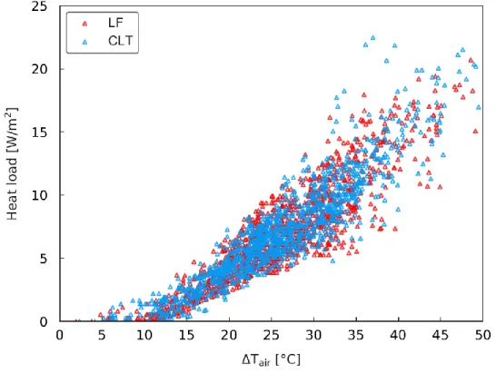
Figure 1.3. Heating load of the building during the heating season (January to April and October to December

2016) as a function of the difference of temperature between indoor and outdoor conditions. ... 23

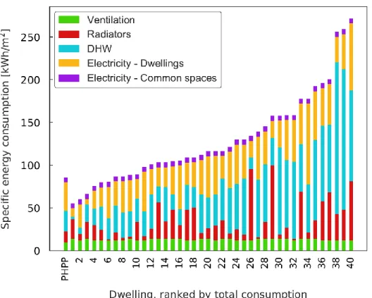
Figure 1.4. Specific energy consumption of the 40 dwellings, ranked from the smallest consumer to the

largest. ... 26

Figure 1.5. Specific heat demand of the dwellings when clustered according to a) their floor, b) the main

orientation of their façade and c) their wall assemblies. ... 28

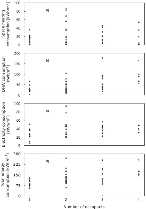
Figure 1.6. a) Heat demand, b) DHW use, c) Electricity use and d) Total energy consumption of a dwelling

according to the household size. ... 29

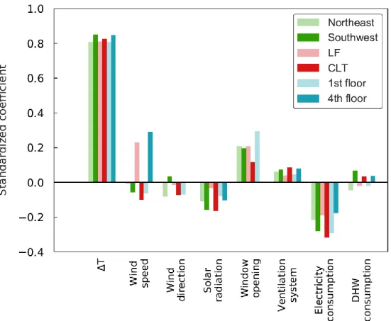
Figure 1.7. Standardized coefficients for each regressor according to the apartment’s orientation of façade,

wall assembly system and floor. ... 36

Figure 1.8. Heat and total energy consumption projected by simulation after applying various modifications

to correct inappropriate hypotheses made during the initial simulation. ... 39

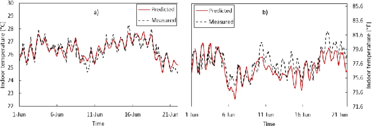
Figure 2.1. Comparison between the indoor temperature and the acceptable range prescribed by ASHRAE

Standard 55 for a) the coldest dwelling and b) the warmest dwelling. ... 52

Figure 2.2. Comparison of simulation from the individual dwelling models and measurements results for the

indoor temperature during the validation period for a) the most accurate model and b) the least accurate model. ... 56

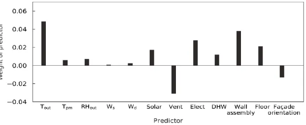
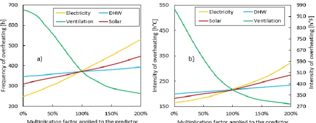
Figure 2.3. Weight of all predictors on the calculations of the indoor temperature. ... 57 Figure 2.4. Impact of the four predictors related to occupant behavior on a) the frequency of overheating and

b) the intensity of overheating. ... 59

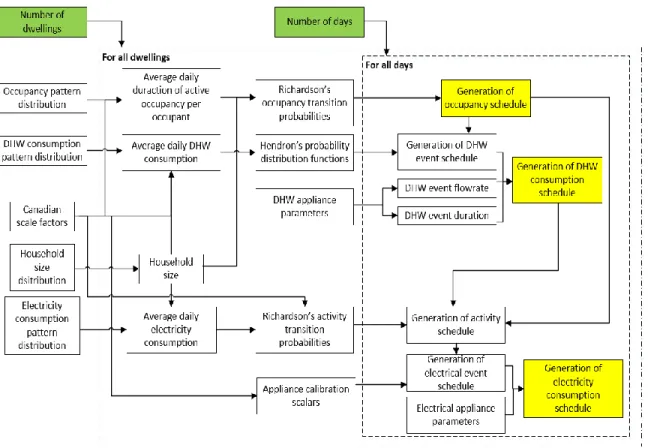
Figure 3.1. Architecture of the occupant behavior model showing the relationship between all components.

Green boxes refer to inputs that have to be provided by the model user. Yellow boxes are the outputs of the model. ... 66

Figure 3.2. Distribution of the average daily amount of time of active occupancy per person in 1,000

simulated dwellings according to different models. ... 69

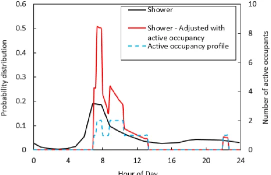
Figure 3.3. Modification made to the probability density function of a shower event to account for active

occupancy. ... 71

Figure 3.4. Aggregated start-time probability density function for the shower before and after accounting for

active occupancy. ... 72

Figure 3.5. Comparison of the measured density of average daily DHW consumption with the one generated

by only considering household sizes. ... 74

Figure 3.6. Distribution of the a) average DHW and b) electricity daily consumption per dwelling obtained

after 100 simulations. Shaded bar represents the cluster in which the monitored building falls into. ... 85

Figure 3.7. Daily a) DHW and b) electricity use by simulated and measured dwellings over a year from one

simulation. Shaded areas represent the range prescribed by the 5th_{and 95}th_{percentiles obtained from the 100}

simulated profiles. a) DHW and b) electricity profiles from 100 simulations compared to the one measured from the case study building. ... 86

Figure 3.8. Average daily a) DHW and b) electricity profiles from 100 simulations compared to the one

measured from the case study building. ... 88

Figure 3.9. Consumption of DHW as a function of household size according to a) measurements and b)

simulations. ... 90

Figure 3.10. a) Average dwelling daily DHW consumption for all measured and simulated profiles (x-axis:

(12)

consumption of a dwelling from measurements and simulations. c) Average dwelling daily electricity consumption for all measured and simulated profiles (x-axis: the 100 profiles, y-axis: the 40 dwellings). d) Inverse cumulative probability function of the DHW consumption of a dwelling from measurements and simulations. ... 91

Figure 3.11. a) Measured and b) simulated day-to-day variability of DHW consumption. ... 93 Figure 3.12. a) Measured and b) simulated day-to-day variability of electricity consumption. ... 94 Figure 3.13. Simulated and measured daily schedule of a) DWH use during the highest day of consumption

b) electricity use during the highest day of consumption and c) electricity us during the lowest day of

consumption for a selected dwelling. ... 95

Figure 4.1. ASHRAE guidelines and actual design (black cross) for the hot water system of the building. . 109 Figure 4.2. Average daily profile of DHW demand for the case study building according to measurements

(full line) and simulations (dashed lines)... 112

Figure 4.3. Schematic representation of the water heater system model used in this paper. The frontier

between cold and hot water in the tank moves according to the amount of hot water. ... 115

Figure 4.4. Hot water system design suggested by the model for different consumption profiles and peak

durations. ... 116

Figure 5.1. Monthly heating demand and number of hours of discomfort for dwelling CLT-N-4 according to

simulated and measured data. ... 132

Figure 5.2. Colormap describing the link between the indoor and outdoor temperature and the probability of

observing an opened window for three apartments in the case study building. ... 135

Figure 5.3. Scatter plot for the window opening behavior in winter and summer for the simulated and

monitored dwellings. ... 138

Figure 5.4. Distribution of a) heating demand, b) total energy use and c) number of hours of discomfort

observed over the 16,000 simulations. ... 140

Figure 5.5. Individual distribution for each simulated dwelling of the a) heating demand, b) total energy use

and c) number of hours of discomfort. Boxes limits represents the first and third quartile of the distribution. Red lines are the medians. Whiskers lengths cover 99.7% of data for a perfect lognormal distribution. Red crosses represent outliers assuming a lognormal distribution... 142

Figure 5.6. Scatter plot of a) the heating demand versus the number of hours of discomfort and b) the total

energy use versus the number of hours of discomfort from stochastic simulations, monitored data and deterministic profiles. ... 143

Figure 5.7. Colormap representing average values of various aspects of occupant behavior within the

Heating-Discomfort two-dimensional plane. ... 144

Figure 5.8. Colormap representing average values of various aspects of occupant behavior within the

Energy-Discomfort two-dimensional plane. ... 145

Figure 5.9. Standardized coefficients for each variables in the heating, energy and discomfort regression

models. ... 147

Figure 5.10. Distribution of a) heating demand, b) total energy use and c) number of hours of discomfort for

housing stocks of 1, 5, 10, 20, 50, 100, 200 and 500 dwellings, along with d) the coefficient of variation of the distribution as a function of housing stock size. The legends in the first three plots display the housing stock size. ... 150

Figure A1.1. Schematic breakdown of the domestic hot water model showing the relationship between all

components. Green boxes refer to inputs provided by the model user. Yellow boxes are the output of the model. ... 178

Figure A1.2. Comparison of aggregated daily active occupancy from Fichardson’s tool before (solid lines)

and after (dashed lines) the suggested adjustement. ... 179

Figure A1.3. Example of probability distribution of a shower event before and after fitting the curve with

(13)

Figure A1.4. Aggregated probability distribution of a shower event before and after fitting the curve with

active occupancy profile. Red and blue curves obtained after 1,000 simulations. ... 183

Figure A1.5. a) Measured and b) Simulated daily DHW consumption in the 39 dwellings during the

validation period. Line within the box shows median day, length of the box shows the 1st_{and 3}rd_{quartile and}

height of whiskers shows 5th_{and 95}th_{percentile. ... 186} Figure A1.6. Effect of the average household size of the building on its DHW demand. ... 187 Figure A1.7. Average daily DHW profile from measurements (full line) compared to the one obtained by the

model, with and without the adjustement for occupancy schedules (dashed lines). ... 189

Figure A1.8. Comparison of simulated data with measurements. Red triangles represent data coming from the

model with adjustment for occupancy schedules and green squares are data coming from the model without the adjustement. Simulated and measured values are in agreement when markers fall on the black line. ... 190

(14)

NOMENCLATURE

Variables

A Surface area [m2_] Cd Discharge coefficient cp Heat capacity [kJ/kgK] cl Clothing factor [clo] CLT Cross-laminated timber CV Coefficient of variation [%]

CV(RMSE) Coefficient of variation of the root mean square error [%] Cvent Cooling rate introduced by ventilation

D Total number of hours of operation [hours]

Davg Discomfort parameter of average temperature [°C]

Dfreq Discomfort parameter of frequency of overheating [hours] Dint Discomfort parameter of intensity of overheating [hours°C] DHW Domestic hot water

DW Durbin-Watson statistic

T

 Difference of temperature [K,°C] Δ t Duration of time [s, min]

E Aggregated energy consumption [Wh] f Mechanical ventilation system use factor g Standard gravity [m/s2_]

h Height above the neutral plane [m] H Window height [m]

HD Heating demand [kWh/m2]

Icons Overall consumption indicator [%]

Idwellings Dwelling-to-dwelling variability indicator [%] Isched Timings of events indicator [%]

IHG Internal heat gains [W] LF Light-frame

m Measured variable

M Annual number of events (Chapitre 4) M Mass of water [kg, lb] (Chapitre 5)

m Mass flowrate [kg/s, lb/min] N Total number of time steps n Number of observations

NHD Number of hours of discomfort [hours] NMBE Normalized mean bias error [%] P Probability

(15)

Greek letters

 Angle of opened window [°]

 _{Density [kg/m}3_]

 Distribution average value  Standard deviation

 Event length [min]

 Daily aggregated amount of time spent on an activity [hours] (Chapitre 4)  Electricity to internal heat gains ratio [WIHG/Welect] (Chapitre 6)

 Regression coefficient related to the dependant variable (Chapitre 3)  Hot water to internal heat gains ratio [WIHG/WDHW] (Chapitre 6)  Logit regression coefficient

 Occupant to internal heat gains ratio [WIHG/occupant]

 Regression coefficient



Regression error  Regression model error

Subscripts

air Indoor and Outdoor air

c Cold Const Constant

clo Closure of windows

DHW Domestic hot water

T

 Difference of temperature

Pon Operating power consumption [W] Q Energy [Wh]

q Heat consumption rate [W, BTU/h] qstack Airflow induced by stack effect [m3/h] qwind Airflow induced by wind [m3/h] R Coefficient of determination [-] s Scale factor (Chapitre 4) s Simulated variable (Chapitre 6) T Temperature [°C, °F]

TEU Total energy use [kWh/m2] U Velocity [m/s]

V Volume [m3, L, gal] Vwind Wind speed [m/s]

V Flow rate [m3/s] W Window width [m]

x Regressors/Independent variable y Dependent variable

(16)

eff Effective

elect Electricity consumption

h Hot

in Inside temperature

loss Storage tank loss op Opening of windows out Outside temperature

peak Consumption peak

q Water heater

rad Solar radiation

tank Storage tank

vent Mechanical ventilation

Wd Wind direction

Ws Wind speed

#Occ Number of occupants

Superscript

- Mean value

(17)

REMERCIEMENTS

J’aimerais tout d’abord dédier cette thèse à ma tante, marraine et amie Sylvie. Malheureusement, Sylvie nous a quittés quelques mois avant la diffusion de ce document. Le courage et la détermination dont elle a fait preuve durant son combat auront été pour moins de puissantes sources de motivation pour l’achèvement de cette thèse. Je sais que Sylvie serait très fière de cette thèse. Je tiens à dire à Serge que nous serons toujours présents pour lui.

Dans un autre ordre d’idée, cette thèse est le fruit de la collaboration de nombreuses parties prenantes dont je me dois de mentionner. Tout d’abord, j’aimerais remercier mon directeur de recherche Louis Gosselin et mon codirecteur Pierre Blanchet. Les deux ont su me superviser durant mon projet afin de m’orienter vers les directions appropriées. Ils ont toujours été en mesure de trouver du temps pour moi malgré leurs horaires chargés. Je les remercie de n’avoir jamais hésité à m’ouvrir des portes et à me faire confiance. Sans eux, ce projet de recherche n’aurait jamais été possible.

Les travaux présentés dans cette thèse sont centrés autour d’un bâtiment multirésidentiel. La construction de ce bâtiment a été mandatée par la Société d’habitation du Québec (SHQ) et il est actuellement opéré par l’Office municipal du Québec (OMHQ). Ces deux organismes ont été des plus présents tout le long du projet et n’ont jamais hésité à répondre à mes questions ou à me fournir les informations demandées. Les entreprises Regulvar, BMD Architectes, Douglas Consultants, Génio Experts-Conseils, Genecor et Poly-Énergie ont également contribué à ce projet en m’offrant accès à leurs données ou leurs plans du bâtiment.

Ce projet a été financé par la chaire industrielle de recherche en construction écoresponsable en bois (CIRCERB) ainsi que par une bourse thématique en énergie octroyée par le Fonds de recherche du Québec – Nature et technologies (FRQNT). L’American Society of Heating, Refrigerating and Air-Conditioning Engineers (ASHRAE) m’a également financé en me remettant un Graduate Student Grant-In Aid Award. Le programme des Bourses canadiennes du jubilé de diamant de la reine Elizabeth II (BRE) et le Bureau international de l’Université Laval (BI) m’ont aussi donné des bourses qui m’ont permis d’effectuer un stage de recherche

(18)

à l’Université de Bath durant l’été 2016. Cette expérience fût des plus enrichissantes, autant d’un point de vue professionnel que personnel. Je tiens à souligner l’apport d’Alfonso Ramallo-González et Sukumar Natarajan qui m’ont supervisé durant ce stage et m’ont donné d’importants conseils qui ont grandement influencé cette thèse.

Je remercie tous les membres du Laboratoire de Transferts Thermiques et d’Énergétique (LaTTE) et du CIRCERB. Les deux groupes sont composés de gens passionnés et ont su construire une ambiance de travail des plus stimulantes et inspirantes. J’aimerais particulièrement mentionner les contributions respectives de Simon et Dominic dans l’avancement de mon projet doctoral. Chez le CIRCERB, j’aimerais souligner la contribution de Natalie Noël, qui s’est retroussé les manches à de nombreuses reprises pendant plusieurs mois en amont à mon arrivée dans le projet pour s’assurer de ce bon lancement. Le technicien Jean Ouellet fut également essentiel au projet par tous les problèmes qu’il a résolu en lien à l’instrumentation du bâtiment étudié. Durant les trois dernières années, Jean et moi avons dû faire des dizaines d’aller-retour au bâtiment pour régler des problèmes avec le système d’acquisition de données. Encore aujourd’hui, Jean craint chacun de mes appels car il présume alors qu’un nouveau problème est apparu.

Enfin, j’aimerais remercier les membres de ma famille rapprochée, soient Ginette, Marie-Josée et Yves. C’est grâce à eux que j’ai pu atteindre le niveau du doctorat. Vous êtes des modèles pour moi et m’avez appris à persévérer, à respecter ses prochains et à demeurer honnête et intègre.

(19)

AVANT-PROPOS

Les divers sujets abordés par cette thèse sont mis en contexte dans le Chapitre 1, qui présente également les objectifs auxquels les travaux de recherche tentent de répondre. Trois publications pour des journaux scientifiques (Chapitres 2, 4 et 5) ainsi que trois articles de conférence (Chapitres 3, 6 et Annexe A1) forment le corps de la thèse. L’article formant l’annexe A1 a été placé en annexe étant donné qu’une importante proportion de sa méthodologie et de ses conclusions sont reprises par l’article situé au sein du Chapitre 4. Les articles présentés dans cette thèse sont listés ci-dessous, avec des informations concernant mes contributions pour chacun d’entre eux ainsi que leur statut de publication.

Chapitre 1 :

J. Rouleau, L. Gosselin and P. Blanchet, “Understanding energy consumption in high-performance social housing buildings: A case study from Canada,” Energy, vol. 145, pp. 677–690, Décembre 2017 (publié).

Notes: Article rédigé par J. Rouleau (moi-même) et révisé par L. Gosselin et P. Blanchet. J’ai effectué le rassemblement des données mesurées utilisées dans cet article en plus de leur analyse. Les modèles de régression linéaire présentés dans l’article ont été développés par moi-même sur Matlab. J’ai aussi effectué l’étude de l’écart de performance énergétique du bâtiment à partir du modèle numérique du bâtiment utilisé durant sa conception. J’ai également dégagé les principales conclusions. Le travail a été réalisé sous la supervision de L. Gosselin et P. Blanchet.

Chapitre 2 :

J. Rouleau and L. Gosselin, “Assessing the risk of overheating in high-performance social housing buildings with the use of regression analysis,” ASHRAE Annual Conference, Houston TX, Juin 2018 (publié).

Notes: Article rédigé par J. Rouleau (moi-même) et révisé par L. Gosselin J’ai effectué le rassemblement des données mesurées utilisées dans cet article en plus de leur analyse. Les modèles de régression linéaire présentés dans l’article ont été développés par moi-même sur Matlab. J’ai également dégagé les principales conclusions. Le travail a été réalisé sous la supervision de L. Gosselin.

(20)

Chapitre 3 :

J. Rouleau, A. Ramallo-González, L. Gosselin, P. Blanchet, and S. Natarajan, “Adapting stochastic occupant behavior models into a unified tool for multi-residential buildings in Canada” Energy Build., Mai 2018 (soumis).

Notes: Article rédigé par J. Rouleau (moi-même) et révisé par l’ensemble des co-auteurs, mais particulièrement par M. L. Gosselin. Cet article se base sur des modèles déjà existants dans la littérature. A. Ramallo-González m’a guidé vers ces modèles. Il rassemble ces modèles en un programme unique qui s’assure de les ajuster pour considérer les différences culturelles entre les pays où ces modèles ont été créés. Des facteurs considérant les différents types d’occupant sont également ajoutés. Tout ce travail de réassemblage et d’ajustements a été effectué par moi-même et a résulté en fonctions sur Matlab que j’ai écrit. J’ai aussi fait la validation des fonctions Matlab écrites. J’ai également dégagé les principales conclusions. Cette publication a été rédigée à partir de travaux effectués lors d’un stage à l’Université de Bath au Royaume-Uni. Le travail a ainsi été réalisé sous la supervision successive de A. Ramallo-Gonzalez et L. Gosselin.

Chapitre 4 :

J. Rouleau, L. Gosselin, and A. Ramallo-González, “Sizing methodology for domestic hot water systems based on simulated occupant behavior”, ASHRAE Annual Conference, Long Beach CA, Juin 2017 (publié)

Notes: Article rédigé par J. Rouleau (moi-même) et révisé par A. Ramallo-González et L. Gosselin. Le concept de dimensionnement des systèmes à eau chaude a été conjointement pensé par L. Gosselin et moi-même. J’ai implémenté ce concept sur Matlab et Excel afin d’obtenir les résultats présentés dans ce texte. L’article se réfère à l’outil de simulation de la demande en eau chaude d’un bâtiment résidentiel que j’ai développé dans le cadre de l’Annexe A1. J’ai également dégagé les principales conclusions. Le travail a été réalisé sous la supervision de L. Gosselin.

(21)

J. Rouleau, L. Gosselin, and P. Blanchet, “Robustness of energy consumption and comfort in high-performance residential building with respect to occupant behavior” Energy, Août 2018 (soumis).

Notes: Article rédigé par J. Rouleau (moi-même) et révisé par L. Gosselin et P. Blanchet. J’ai créé les modèles de bâtiments dans TRNSYS en plus des codes MATLAB nécessaires pour utiliser en boucle les modèles TRNSYS. Les modèles de bâtiments utilisent l’outil de simulation des occupants que j’ai développé dans le cadre du Chapitre 4. À cet outil se rajoute un modèle d’ouvertures de fenêtre qui a été par moi-même. Je me suis occupé de la calibration et validation des modèles TRNSYS ainsi que de l’analyse des résultats de simulation. J’ai également dégagé les principales conclusions. Le travail a été réalisé sous la supervision de L. Gosselin et P. Blanchet.

Annexe A1 :

J. Rouleau, A. Ramallo-González, and L. Gosselin, “Towards a comprehensive tool to model occupant behavior for dwellings that combines domestic hot water use with active occupancy”, ASHRAE Annual Conference, Long Beach CA, Juin 2017 (publié)

Notes: Article rédigé par J. Rouleau (moi-même) et révisé par A. Ramallo-González et L. Gosselin. Cet article se base sur des modèles déjà existants dans la littérature, qui m’ont été fourni par A. Ramallo-González. Il rassemble ces modèles en un programme unique qui s’assure de les ajuster pour considérer les différences culturelles entre les pays où ces modèles ont été créés. Tout ce travail de réassemblage et d’ajustements a été effectué par moi-même et a résulté en fonctions sur Matlab que j’ai écrit. J’ai aussi fait la validation des fonctions Matlab écrites. La rédaction de cet article a été faite dans le cadre d’un stage à l’Université de Bath au Royaume-Uni. Le travail a ainsi été réalisé sous la supervision successive de A. Ramallo-Gonzalez et L. Gosselin.

(22)

Les seules modifications apportées aux articles insérés par rapport à leurs versions publiées ont été le changement de numérotation des équations, des tables et des figures. Aucun changement en lien au contenu n’a été apporté.

(23)

INTRODUCTION

Mise en contexte

Le citoyen moyen en Amérique du Nord passe plus de 90% de son temps au sein d’environnements intérieurs, que ce soit pour y vivre, y travailler, socialiser ou autres activités [1]. Les bâtiments sont attrayants puisqu’ils nous offrent un environnement confortable en nous protégeant des intempéries météorologiques et autres facteurs extérieurs. En hiver, nous apprécions la chaleur de nos maisons alors que durant les canicules en été, nous courrons les édifices ayant de l’air climatisé. Toutefois, ce confort offert par nos bâtiments ne tombe pas du ciel, car de l’énergie doit nécessairement être dépensée pour assurer le niveau de confort désiré. Cette énergie consommée a des retombées sur l’environnement, principalement par l’émission de gaz à effet de serre dans l’atmosphère.

C’est pour cette raison que le secteur du bâtiment représente un point névralgique de la lutte contre les changements climatiques. En effet, les bâtiments demandent 36% de l’énergie totale consommée sur la planète et cette consommation engendre 39% des émissions de gaz à effet de serre dans l’atmosphère [2]. La dépendance énergétique des bâtiments est un enjeu important et la réduction de cette dépendance demande aux professionnels œuvrant dans le domaine de se retrousser les manches. Ce constat explique les objectifs ambitieux d’efficacité énergétique que se sont fixés la plupart des organismes liés au domaine. Nous pouvons penser par exemple à l’ASHRAE qui souhaite être en mesure d’établir des bâtiments net zéro (bâtiments produisant autant d’énergie qu’ils en consomment) viables financièrement d’ici 2030 [3].

Pour améliorer l’efficacité énergétique des bâtiments, les bâtiments résidentiels sont particulièrement intéressants parce qu’ils forment la principale cause derrière les pointes journalières de consommation énergétique que les réseaux énergétiques subissent [4]–[6]. Chaque matin et chaque soir, la puissance énergétique consommée par une communauté augmente drastiquement puisque les gens sont à la maison et consomment par toutes sortes de manières plus d’énergie (douche, préparation des repas, télévision…). Parfois, il arrive que le fournisseur d’énergie ne soit pas en mesure de répondre par ses propres moyens à la

(24)

demande des clients et qu’il importe donc de l’énergie provenant de sources plus dispendieuses et moins écologiques. Par exemple, dans le contexte québécois, lors des moments de grandes demandes en puissance se produisant au plus froid de l’hiver, il arrive à Hydro-Québec de devoir importer de l’électricité produite hors de son réseau. Cette électricité est habituellement produite à partir de combustibles fossiles non renouvelables et est fournie par l’exportateur à haut prix. L’amélioration de la performance énergétique des bâtiments résidentiels a ainsi un double effet puisqu’en plus de réduire la consommation globale d’énergie de la société, la gestion de ces pointes journalières de puissance consommée est facilitée.

Pour optimiser l’efficacité énergétique des bâtiments résidentiels, il faut posséder une bonne compréhension de la consommation énergétique de ces derniers. La simulation énergétique de bâtiments représente un puissant outil pour approfondir notre compréhension. L’emploi de logiciels de simulation (eQuest, TRNSYS, EnergyPlus, PHPP…) permet de projeter les besoins en énergie de plusieurs configurations d’un bâtiment donné selon divers scénarios. L’utilisateur peut ainsi choisir un design de bâtiment qui mènera à une faible demande en énergie. Cependant, il s’avère fréquent que la consommation réelle d’un bâtiment diverge de ce qui avait été prévu par un tel outil de simulation, un phénomène nommé « l’écart de performance énergétique » [7]–[9]. En effectuant une revue de la littérature, van Dronkelaar et al. ont trouvé que l’écart de performance énergétique moyen d’un ensemble de 62 bâtiments de tout genre était de +34% (sous-estimation de la consommation réelle) avec un écart-type de 55%, montrant l’amplitude de ce phénomène [10].

Cet écart entre la prédiction et la réalité s’explique par le fait que la simulation énergétique de bâtiments fait appel à de nombreuses hypothèses qui peuvent influencer le résultat de la simulation. Tronchin et Fabbri ont essayé de prédire la consommation d’une maison unifamiliale en Italie en employant trois méthodes de calculs distinctes. Ils ont noté que les trois méthodes menaient à un écart de performance significatif, mais aussi que les niveaux de consommation prévus variaient selon la méthode de calcul employé [11]. Jones en est venu à des conclusions semblables lorsqu’il a demandé à six étudiants gradués de créer

(25)

leur propre modèle d’un édifice à appartements [12]. Les prédictions de consommation énergétiques de bâtiments résidentiels sont donc très sensibles à la méthode de calcul et aux hypothèses utilisées.

Ces hypothèses se rattachent non seulement aux variables physiques du bâtiment (enveloppe, systèmes mécaniques…) et aux conditions météorologiques, mais également au comportement des occupants [13]–[15]. Le comportement des occupants est défini comme étant l’ensemble des gestes posés par une personne qui peut avoir un effet sur la demande en énergie et le confort thermique d’un bâtiment. Puisque le comportement des gens au sein de leur logement varie jour après jour et qu’il est différent d’un logement à l’autre, il possède un caractère hautement probabiliste qui le rend très difficile à représenter dans le cadre de simulations énergétiques. C’est particulièrement le cas pour les bâtiments résidentiels puisque les occupants ont moins de contraintes pouvant limiter leurs actions au sein de leur logement.

Or, le comportement des occupants peut fortement affecter la consommation d’un bâtiment [16]. En effectuant une analyse de sensibilité des paramètres affectant le plus la demande de chauffage d’un bâtiment résidentiel au Pays-Bas, Ioannou et Itard ont remarqué que les incertitudes sur les variables reliées aux occupants avaient beaucoup plus d’importances que celles des variables reliées aux systèmes du bâtiment [17]. Dans l’ensemble, il a été démontré que des habitudes d’opération de bâtiment non énergétiquement efficaces pouvaient augmenter la demande en chauffage d’un bâtiment par un facteur d’au moins deux [18]. De plus, avec l’amélioration constante de la qualité des bâtiments, l’impact des occupants devient de plus en plus important dans le bilan énergétique d’un bâtiment [19]. Il devient essentiel de bien représenter les occupants lors des simulations énergétiques de bâtiments pour améliorer leurs prédictions par rapport à la performance du bâtiment étudié.

C’est donc autour de sujets tels que la performance énergétique des bâtiments résidentiels, les simulations et leurs écarts de performance énergétique et le rôle joué par les occupants que cette thèse est articulée. La thèse se concentre sur les bâtiments ayant une structure de bois. Puisqu’il s’agit d’un matériau à faible impact environnemental, le bois se présente

(26)

comme étant un matériau de l’avenir pour le domaine de la construction; pour cette raison, il est important de saisir comment des bâtiments basés sur ce matériau se comportent d’un point de vue énergétique. La thèse se base ainsi sur l’instrumentation et le suivi d’un bâtiment en bois de logements sociaux, qui porte le nom de Les Habitations Trentino. Situé dans la ville de Québec, ce bâtiment est un outil de démonstration mis en place par la Société d’Habitation du Québec (SHQ) pour montrer la faisabilité et la rentabilité des bâtiments à faible consommation énergétique. Différentes mesures ont ainsi été implantées pour diminuer les besoins en chauffage du bâtiment; ces mesures seront décrites au fil des chapitres de cette thèse. Les Habitations Trentino ont aussi la particularité d’être composées de deux structures distinctes de bois. L’analyse des données provenant de ce bâtiment réellement opéré sont au centre de cette thèse et apportent à la communauté de l’information inaccessible par les méthodes conventionnelles de la simulation énergétique.

Objectifs

L’objectif principal de cette thèse est d’approfondir notre compréhension de la consommation énergétique et du confort thermique des bâtiments résidentiels en bois à haute performance énergétique. Le but est d’identifier des pistes de solutions favorisant l’amélioration de l’efficacité énergétique de tels types de bâtiments. Étant donné le grand rôle qu’ils ont à jouer, ces solutions se concentreront principalement sur les occupants et leur comportement à domicile. Pour ce faire, cette thèse est centrée autour des axes de recherche suivants :

1. Le suivi assidu de la performance énergétique d’un bâtiment multirésidentiel dans le but de comprendre concrètement son comportement énergétique.

2. L’élaboration d’un modèle stochastique de comportement des occupants dans des bâtiments résidentiels en rassemblant des outils disponibles dans la littérature.

3. L’étude de l’influence des occupants sur la performance d’un bâtiment résidentiel en bois en considérant la diversité inter-ménage du comportement des occupants lors de la phase de conception du bâtiment.

(27)

Des objectifs spécifiques sont reliés à chacun de ces trois axes, tel que décrit dans les sous-sections 1.2.1 à 1.2.3. Trois articles de journaux scientifiques et trois articles de conférence ont été rédigés dans le but de répondre à ces objectifs. Les sections 1.2.1 à 1.2.3 révèlent également à quels chapitres de la thèse chaque axe de recherche est associé.

Axe 1: Suivi de la performance d’un bâtiment multirésidentiel

Une évaluation post-occupationnelle d’un bâtiment est un exercice fort utile pour bien comprendre le comportement thermique d’un bâtiment. Par l’analyse de données, elle permet d’établir différentes corrélations permettant d’estimer les besoins en énergie et le confort thermique d’un bâtiment. Les Chapitres 2 et 3 se basent sur une telle évaluation afin de répondre aux objectifs spécifiques suivants :

1.1 Comprendre où l’énergie des bâtiments à haute performance est consommée et quels sont les principaux facteurs d’influence de cette consommation.

1.2 Étudier la présence potentielle d’un écart de performance énergétique et si écart il y a, l’expliquer.

1.3 Analyser la possibilité de construire des modèles statistiques permettant de prévoir la consommation d’énergie et le confort thermique d’un bâtiment.

1.4 Comparer avec des données in-situ la performance thermique d’un bâtiment avec une structure légère en bois versus celle d’un bâtiment utilisant une structure massive. 1.5 Évaluer le potentiel que la ventilation naturelle possède pour contrôler les températures intérieures estivales d’un bâtiment à haute performance énergétique.

Axe 2 : Élaboration d’un modèle stochastique des occupants

Étant donné leur grande importance, il est crucial de représenter fidèlement les occupants lors des simulations énergétiques des occupants. La littérature scientifique se concentre donc de plus en plus sur la création de modèles stochastiques du comportement des occupants pour mieux saisir son aspect probabiliste. Le Chapitre 4 (ainsi que l’Annexe A1) présente un outil centralisateur de modèles déjà existants qui a été développé dans le but

(28)

de pouvoir simuler les différents types d’occupants. Cet outil a été construit pour atteindre ces objectifs :

2.1 Centraliser différents modèles touchant à un seul aspect du comportement des occupants en un outil unique.

2.2 Considérer la diversité de comportement inter-ménage lors de la simulation énergétique de bâtiments résidentiels.

2.3 Adapter des modèles de comportement conçus outremer au mode de vie canadien. 2.4 Évaluer l’effet des modifications apportées sur les profils d’occupant générés.

Axe 3 : Étude de l’influence des occupants sur les bâtiments résidentiels

Le troisième axe de recherche profite de l’outil développé lors du deuxième axe pour évaluer l’impact que les occupants ont sur la performance énergétique d’un bâtiment à haute performance énergétique. Cette évaluation est couverte par les Chapitres 5 et 6. À mesure qu’on améliore les systèmes des bâtiments pour les rendre de plus en plus efficaces, on se rend de plus en plus compte de la grande importance que les occupants ont. Cet axe de recherche s’intéresse à quantifier cette importance autant pour la performance d’un bâtiment résidentiel que pour le dimensionnement de ses systèmes. L’axe 3 tente spécifiquement de répondre aux tels objectifs :

3.1 Quantifier l’impact global des occupants sur la performance énergétique d’un bâtiment.

3.2 Isoler l’influence des différents aspects du comportement des occupants (température de consigne, consommation d’eau chaude…).

3.3 Évaluer l’intérêt de considérer l’aspect stochastique du comportement des occupants lors des simulations de bâtiment.

3.4 Comprendre comment la représentation des occupants lors de la phase de conception d’un bâtiment peut affecter le dimensionnement de ses systèmes.

(29)

UNDERSTANDING ENERGY CONSUMPTION IN

HIGH-PERFORMANCE

SOCIAL

HOUSING

(30)

Résumé

Cet article présente le suivi énergétique d’un bâtiment de logements sociaux à haute performance énergétique. Le but est de comparer les niveaux de consommation d’énergie prédits et réels ainsi que d’identifier les paramètres ayant le plus d’influence sur les besoins en énergie. Un système d’acquisition de données enregistre des mesures prises sur le bâtiment à une fréquence de 10 minutes. Le bâtiment étudié a la particularité d’être composé de deux sections symétriques utilisant des systèmes structuraux en bois distincts. Aucune différence notable de consommation d’énergie est détectée entre les deux parties du bâtiment. Toutefois, une grande variabilité est observée lorsqu’on compare la consommation individuelle de chacun des logements et ce, peu important leur structure. L’impact de l’orientation du logement semble minimal par rapport à cette variabilité, ce qui suggère que le comportement des occupants est le facteur dominant qui explique la variabilité inter-ménage de consommation. Des analyses de régression linéaire montrent que certains aspects du bâtiment qui sont contrôlés par les occupants, comme l’ouverture de fenêtres en hiver ou l’utilisation d’appareils électriques, ont un grand impact sur le bilan énergétique des logements. En 2016, l’écart de performance énergétique entre la consommation prévue pour le bâtiment et celle mesurée était de 74%. Les données récoltées sur le bâtiment ont permis d’identifier les causes de ce grand écart.

(31)

Abstract

This paper presents a case study of a recently built high-performance Canadian social housing building with the aim of comparing the expected and measured energy consumptions and to identify the parameters affecting the most the energy need. A monitoring system compiles at a 10-minute frequency information related to the energy use and the thermal conditions observed in the building and its HVAC system. The building has the particularity of comprising two symmetric sections made of different timber structure systems. No significant differences of energy consumption were detected between the two parts of the buildings. However, a large variance was observed when comparing each dwelling individually regardless of their structures. The orientation of the dwelling also exhibited a minimal influence compared to these variations, suggesting that occupant behavior is the dominant factor explaining dwelling-to-dwelling variability and is thus critical for understanding energy use in residential buildings. Regression analysis showed that specific occupant actions, such as opening windows in winter or using electrical appliances, have a great impact on the energy balance of the apartments. In 2016, the performance gap between measured and expected total energy demand of the building was 74%. With the use of the large dataset coming from the building, it was possible to determine the causes behind this large gap for the reference building.

(32)

Introduction

Improving the energy performance of buildings represents a crucial component for achieving a more sustainable management of energy. 40% of the energy consumed in the US is used by buildings [20] and a similar proportion is observed in Europe [21]. Consequently, building-related stakeholders such as the American Society of Heating, Refrigerating and Air-Conditioning Engineers (ASHRAE) or the European Performance of Buildings Directive (EPBD) have established ambitious objectives for the next 15 years. For example, the goal that ASHRAE is attempting to establish is to produce market-viable Net Zero Energy Buildings (NZEBs) by 2030 [22]. Similarly, the EPBD wants new buildings in 2020 to be close to this NZEB target [23].

A great understanding of building physics is necessary to accomplish these tasks since improving a design becomes more and more difficult as buildings get more efficient. Buildings are complex systems, the energy performance of which involves heat and mass transfer through the envelope, windows characteristics, ventilation strategy, solar radiation, internal gains, decision-making of the occupants, efficiency of the HVAC systems, and so on. Identifying the most effective ways to reduce energy consumption in buildings is thus not trivial. It is particularly the case for residential buildings due to the high diversity of occupant behaviors observed in such buildings, leading to large variations of energy demand even between very similar buildings [24]. Since people spend the majority of their time at home, residential buildings play an important part in the energy demand and are responsible for peak demands incurred by energy providers. As a result, residential buildings have a distinct contribution within the building sector.

In-situ evaluation of building energy performance is helpful for increasing our knowledge on building physics and are critical for energy saving analyses. Data obtained during the assessment of a building performance has been used to accurately depict energy consumption for supermarkets [25], residential [26]–[28], commercial [29], [30] and office [31] buildings. For example, Kneifel and Webb were able to build a regression model for NZEBs that provide a viable baseline for evaluating energy consumption comparable to a

(33)

traditional simulation model, but with far lower computational efforts [32]. Such models allow the direct quantification of the impact of various parameters (indoor and outdoor temperatures, solar radiation…) on the energy consumption of a building. For residential buildings, Catalina et al. proved with a regression analysis that the shape of the building and its thermal inertia have a significant impact on its energy demand [26]. Measured data can even be used in regression analysis to quantify impacts of social factors on energy consumption as revealed by Chen et al. who found that resident age has a larger influence than their income [33].

Another reason to record data from real buildings is related to a major weakness of currently used numerical models – their lack of accuracy. An important energy performance gap (EPG) is typically seen between the actual energy consumption of a building and the one predicted by numerical simulations [34]–[37]. In a study covering more than 950 homes, Tronchin and Frabbi estimated the energy demand of a house using different methodologies which all yielded energy performance gaps, demonstrating that the gap is present regardless of the computational method [38]. Jones obtained a similar conclusion when he asked six graduate students to create their own model for an apartment building without consulting each other [39]. The six models had completely different predictions for the building annual energy consumption (ranging from 2,654 to 4,292 kWh) that were all far from the true demand (2,170 kWh). The energy performance gap is thus not only caused by the computational method or simulation software, but also by the modelers themselves. Building simulations require a vast quantity of input parameters that usually need to be approximated. Inadequate decisions on these parameters and poor awareness of their impacts of the simulations results lead to predictions that are off [40]. Measured data can be used to calibrate models in order to circumvent this lack of accuracy. The lack of available data for model calibration can be a problem for building simulations [41]. Without validation, numerical models cannot be employed to their full potential.

Studies in the past have relied on numerical methods based on energy modeling to quantify drivers of energy use in buildings, usually by adopting a bottom-up approach [42]–[45]. Liu et al. for instance used sensitivity analysis to assess the importance of meteorological

(34)

parameters in building energy consumption [46]. They found that temperature had the strongest effect on both heating and air conditioning energy use and that global solar radiation did not directly affect building energy demand. Except for the relative humidity, the weather variables were more important for heating in winter than for air conditioning in summer. A similar procedure was applied on the occupant actions in a Passivhaus dwelling which revealed that the set point temperature, the use of electrical appliances and the ventilation behavior all influence heating demand [47]. An artificial neural network trained with building models supports the findings of the previous study in that it estimated that in an airtight and well-insulated building, reducing the set point from 22 to 20°C could decrease by approximately 35% the need of heating [48]. Occupancy of a residential building is another important parameter as there is a direct link between energy consumption of a dwelling and the occupancy patterns of its household [49]. These studies demonstrate the impact of occupant behavior and of weather on the energy demand of a residential building, but they are based on numerical building models that are not always fully validated. It would be beneficial to research similar aspects by employing a top-down approach that is entirely based on measurements coming from real buildings.

Although literature contains a vast amount of studies in which residential buildings were experimentally evaluated, a limited number of assessments of multi-residential buildings is found. Although the energy performance gap was generally observed in these studies. Since occupants are difficult to model in multi-residential buildings due to the high number of households, occupant behavior is usually suspected to be the main culprit behind the energy performance gap that is generally observed in these studies. Nonetheless, to the knowledge of the authors, no thorough analysis has been made in apartment buildings to confirm the sources of the energy performance gap. For instance, Calì examined the discrepancy between expected and observed energy consumption of three apartment buildings following refurbishment during four successive years [50]. The relative difference between expectations and observations during these years varied from 41% to 117%. These differences were explained by technical issues (distribution losses of the DHW system in this case) and occupant behavior. Calì then used data recorded during his study to quantify the impact of the set point temperature and of the average window

(35)

position on the heating energy consumption. It was found that while the former has a moderate impact, the latter surprisingly has no tangible impact on a dwelling’s consumption. However, when evaluating the energy performance gap, Calì was unable to separate the role of the occupants and that of the technical issues and thus could not quantify the impact of occupant behavior on the EPG. In another study, the impact of occupant behavior was also easily observable in an apartment building in Italy [51], [52]. In the sample of 196 apartments contained in this building, the heat consumption of each dwelling during a winter season ranged from 0.0 to 62.4 kWh/m2_{in spite of high similarity} of the dwellings. Similar variation was seen for domestic hot water (DHW) consumption (50 to 350 L/day per dwelling) and summer cooling demand (0 to 56 kWh/m2). Preliminary analyses made by the authors suggested that the number of occupants and the heating and cooling set point temperatures, all variables that depend on occupancy, could be behind these differences, but in-depth study was made to confirm the significance of these parameters.

The present paper analyzes the energy demand of a high-performance social housing building that has been thoroughly monitored in real-time since 2015. Various aspects, such as window openings, indoor temperatures and DHW consumption, are measured in addition to the heating energy demand of each apartment. The building is described in Section 2, along with the energy modeling done during the design phase and the monitoring system that has been installed. Section 3 presents different thermal patterns found during the evaluation of the building energy performance. This is followed in Section 4 by a regression analysis that is done to assess which parameters drive the heat consumption in winter. Finally, the paper ends with a study on the energy performance gap where the pre-construction model of the building is explained using post-occupancy data. In this manner, the influence of each erroneous hypotheses could be quantified. In short, the aim of this paper is to use a case study building to increase our understanding of multiresidential buildings physics in order to help reduce energy performance gaps in the future.

(36)

Monitoring of the case study building 1.2.1.1 Case study building

The monitored building is a recently built multiresidential social housing building located in Quebec City, Canada. Most of the 40 dwellings located in the building are inhabited by young families – the population’s mean age is 26.6 years old. For the sake of comparison, the average age of the population of Quebec City in 2016 was 43.2 years old [53]. A total of 90 people (2.25 per residential unit) live in the building. It was built with the objective of serving as a demonstration of the practicability and profitability of high-performance social residential buildings in the Province of Quebec. Its design drew heavily on the Passivhaus approach: it has a compact shape (surface-to-volume ratio of 0.28 and form heat loss factor of 1.14) and a highly insulated envelope (U-values of 0.157 W/m2K for vertical walls and 1.15 W/m2K for windows) to reduce heat losses, a continued insulation to minimize thermal bridges and a high airtightness (0.6 air change per hour at 50 Pa) to limit infiltrations. In addition to heat-recovery ventilator units recovering up to 85% of the exhaust air thermal energy, solar walls were installed to preheat outdoor air during the heating season. The ventilation system has a total capacity of 4,000 m3_{/h. It is a 100% fresh} air system in which the primary air is only tempered, i.e. most of the heating is provided by radiators in each dwelling. Note that the occupants in each dwelling have access to their own on/off switch for the ventilation system. A district heating hot water loop provides the required heat for the building, via heat exchangers. The thermal energy of the district system is transferred to all dwellings for space heating by ventilation and radiators. Domestic hot water is also obtained by using heat from district heating. Occupants do not receive separate bills for thermal energy as it is already included in their lease (electricity however is not included in the lease, so each household has its own electricity meter). In summer, there is no mechanical system to cool the air – overheating is controlled solely by natural ventilation. The reference building is presented in more detail in Table 1.1, which summarizes the characteristics of the case study building, and Fig. 1.1, which offers a visual depiction. In the floor plan, dwellings in green have light-frame wall assemblies whereas yellow dwellings use a CLT structure.

(37)

Table 1.1. Characteristics of the building envelope and HVAC system chosen during the design phase.

Type of structures CLT LF

Treated floor area [m2_]

3024.50

Exterior wall area above grade

[m2_]

1672.9

Exterior wall area below grade [m2_] 114.58 Roof area [m2_] 773.20 Ue (Exterior walls) [W/m2_K] 0.158 0.157 Ur (Roof) [W/m2_K] 0.138 0.107 Us (Floor slab) [W/m2_K] 0.539 Ub (Basement walls) 0.301

Fenestration type Triple glazing, low-E, Argon Ug (Glazing) [W/m2_K] 0.790 Uf (Window frame) [W/m2_K] 1.330 Window-to-wall ratio 16.0% g-value 0.56 Ventilation average air change rate

[1/h] 0.41 Ventilation heat recovery efficiency 85% Ventilation electric efficiency [kJ/m3_] 3.1

Air change rate at pressure test [1/h]

(38)

Figure 1.1. a) Northeast façade of the building and b) Floor plan of the building.

One side of the building employs light-frame wall assemblies (LF) for the structural system, whereas the other side relies on massive timber panels (cross-laminated timber (CLT)). This particular use of two constructive systems in the same building was specifically chosen to compare their energy performance and the easiness and cost of their implementation. Quebec’s construction traditionally uses wooden light-frame for residential buildings. It has the advantage of being an economical structure in terms of capital and materials. However, light-frame wall assemblies cannot be used for buildings over six stories, hence the appeal of CLT, an engineered building system with superior structural properties than light-frame structures. A barrier for the growth of CLT in North