Method for evaluating an extended fault tree to analyse the dependability of complex systems: application to a satellite-based railway system

OATAO is an open access repository that collects the work of Toulouse

researchers and makes it freely available over the web where possible

Any correspondence concerning this service should be sent

to the repository administrator: tech-oatao@listes-diff.inp-toulouse.fr

This is an author’s version published in: http://oatao.univ-toulouse.fr/19979

To cite this version:

Nguyen, Thi Phuong Khanh

and Beugin, Julie and Marrais,

Juliette Method for evaluating an extended fault tree to analyse the

dependability of complex systems: application to a satellite-based

railway system. (2014) Reliability Engineering and System Safety

(133). 300-313. ISSN 0951-8320

Official URL: http://dx.doi.org/10.1016/j.ress.2014.09.019

Open Archive Toulouse Archive Ouverte

Method for evaluating an extended Fault Tree to analyse the

dependability of complex systems: Application to a satellite-based

railway system

T.P. Khanh Nguyen

, Julie Beugin

, Juliette Marais

b_{Univ Lille Nord de France, IFSTTAR, COSYS, LEOST, Villeneuve d'Ascq, France}

Keywords:

Dynamic & time dependent Fault Tree Repairable & multi-state components Petri net modelling

Monte Carlo simulation Dependability analysis GNSS-based localisation unit

a b s t r a c t

Evaluating dependability of complex systems requires the evolution of the system states over time to be analysed. The problem is to develop modelling approaches that take adequately the evolution of the different operating and failed states of the system components into account. The Fault Tree (FT) is a well-known method that efficiently analyse the failure causes of a system and serves for reliability and availability evaluations. As FT is not adapted to dynamic systems with repairable multi-state compo-nents, extensions of FT (eFT) have been developed. However efficient quantitative evaluation processes of eFT are missing. Petri nets have the advantage of allowing such evaluation but their construction is difficult to manage and their simulation performances are unsatisfactory. Therefore, we propose in this paper a new powerful process to analyse quantitatively eFT. This is based on the use of PN method, which relies on the failed states highlighted by the eFT, combined with a new analytical modelling approach for critical events that depend on time duration. The performances of the new process are demonstrated through a theoretical example of eFT and the practical use of the method is shown on a satellite-based railway system.

1. Introduction

In order to satisfy user requirements, the configuration of technical systems becomes more and more complex and is the combination of multiple sub-systems. In the railway context for example, the Global Navigation Satellite System (GNSS) is an advantageous solutions for on-board localisation units as it offers an interoperable worldwide solution and as it reduces infrastructure costs. However, numerous studies[1,7]emphasised the necessity of reinforcing the performances of GNSS localisation units by other sensors when they are used in safety applications. Numerous combinations between GNSS and other kinds of sensors, such as odometer/ tachometer, Inertial Navigation System (INS) or Eddy Current Sensor (ECS) are considered. In this context, the GaLoROI project (Galileo Localisation for Railway Opera-tion InnovaOpera-tion), which aims at developing a certifiable, safety-relevant, and satellite-based localisation unit for low density railway lines, is ongoing. The operation principle of GaLoROI is to combine satellite positioning data with satellite-independent data, here pro-vided by an ECS. This combination poses multiple challenges when

analysing and evaluating the system dependability. In fact, it is necessary to provide an efficient analysis method that can evaluate the behaviour of complex systems.

Using popular, simple and standard notation, the Fault Tree (FT)

[6]method provides an ideal framework for deductive analyses of

causal relationships between a system fault and associated failure events. It also allows the calculation of probabilities related to the combinatorial logic of several associated gates. Therefore, it is suitable for both qualitative, quantitative analyses and is widely used in reliability and safety studies. For example, a recent study

[25] uses the FT approach with customer weighted values of

component failures frequencies and downtimes for predicting customer reliability of a distribution power. However, FT analysis is based on the assumption that all components must be in boolean state (working or failed) and that component failure events are pairwise stochastically independent. These assump-tions allows the evaluation of the system unreliability using the combinatorial method but is not sufficient to capture real beha-viours of complex systems.

By defining additional gates, an extension of the FT, called

Dynamic Fault Tree (DFT), was first proposed in [5] to attain a

higher level of system dependability analysis. This method that was

then developed in numerous studies [2,18,10,19,26]allows failure

sequences, functional dependent failures and presence of spare E-mail addresses: khanh.nguyen@ifsttar.fr,

nguyenthipk85@gmail.com (T.P.K. Nguyen), julie.beugin@ifsttar.fr (J. Beugin),

components to be captured. However, these studies do not consider the components having multi-states due to degradation processes and time conditions of the causes that lead to critical consequences.

Refs.[4,11,12]presented another extended FT, called multi-state

Fault Tree (mFT). This mFT allows considering degraded compo-nents whose states are stochastically dependent and also allows

taking into account the repair events[4].

On the other hand, extensions of FT with time parameters (time conditions of event duration that lead to critical consequences, delay time between cause and effect) are useful for the dependability

analysis of technical systems. Ref.[22]expressed quantitative time

relations between causes and effects by defining numerous addi-tional temporal gates. This extension is called Temporal Fault Tree

(TFT). Ref.[13]also considered the time relation between causes and

effects using State-Event Fault tree (SEFT). For this extended FT, inputs of gates are both instantaneous events and states that last over a period of time. It allows addressing dynamic behaviours that depend on event sequences and considers the duration time conditions of

events. Ref.[15] presented Time dependencies Fault Tree (TdFT) and

focused on the timing analysis of the hazard events. In this last paper, events are not considered as instantaneous but are expressed by their duration times. The authors then define the causal gates characterised by the delay times between causes and consequences. For dependability analysis of complex technical systems, such as the GaLoROI localisation system, it is necessary to provide an efficient method that permits to:

1. consider the repairable multi-state components,

2. take into account sequence dependent behaviours of a system, 3. examine duration conditions of the causes that lead to critical

events.

Therefore, we follow the research directions of[2,4,5,13,15,22] and

present in this paper the extended Fault Tree (eFT) that combines advantages of these above FT models for qualitative dependability analysis. In order to find the most appropriate method for evaluating this eFT, a survey of existing methods is examined inSection 2. After a discussion, the necessity for developing a new evaluation process, which is based on the Petri net (PN) modelling of critical events due to

the duration of degraded states of sub-system, is highlighted. This

modelling process is presented inSection 3and is performed by two

steps:

1. An analytical approach is developed in order to directly calculate the probability distribution function (pdf) of critical events stemming from the duration of a particular state. 2. Based on the pdf, an algorithm is proposed to sample the

occurrence time of these critical events.

Then, the last part ofSection 3aims at proving the accuracy and at

showing the efficiency of our new evaluation process. Moreover, the performance of our approach is illustrated one more time when

considering a practical example, the GaLoROI system in Section 4.

Finally, Section 5presents the conclusion and the further research

works.

2. Methods for evaluating extended Fault Trees

2.1. Overview of existing methods for evaluating the Fault Trees and extended Fault Trees

Two main approach types are employed in order to evaluate the FT and its extensions:

1. Analytic approaches aim at giving precise and reliable results, but it is not enough efficient for taking into account multiple complex behaviours of systems.

2. Modelling and simulation approaches aim at capturing the behaviours of complex systems, but their results are less precise.

2.1.1. Analytic approaches

2.1.1.1. Combinatorial methods for evaluating mFT. As long as there are no additional stochastic interdependencies between the com-ponents, the multi-state Fault Tree (mFT) can still be qualitatively analysed using the combinatorial methods. In earlier studies

[11,12], the authors extended the combinatorial method of FT. For that, they defined discrete function characterising the relations between inputs and outputs of combinatorial gates in order to quantitatively analyse mFT. This method is only appropriate for a static system, i.e. a system that is examined without considering the possible evolution of its states over time.

2.1.1.2. Methods for evaluating DFT. When considering stochastic interdependencies between components, such as the order in which stochastic fault events occur, the combinatorial models are not appropriate. In order to quantitatively evaluate a DFT,[5,19]generate all the possible system states and stochastic transitions between states, i.e. the Continuous Time Markov Chain (CTMC) of the system. This is an efficient method to examine the dependencies of stochastic events or component states. However, this method presents the following drawbacks:

1. the number of basic events of the DFT can lead to an explosion of the state space of the CTMC.

2. the analytic evaluation is based on the assumption that all transi-tions between states follow exponential probability distributransi-tions. 3. it is difficult to take into account the maintenance information.

In order to reduce the state space explosion problem of CTMC,[10]

presented a modular approach for identifying and solving the independent sub-trees. This approach is appropriate for fault trees whose a small part is dynamic in nature. Different techniques are applied to each sub-tree depending on its characteristics (static or dynamic) and the solutions are integrated to get the results for the

Notation in this paper.

S State space of the component

i Degraded state whose the sojourn time that satisfies duration time condition can lead to a critical event (CE)

n Number of sojourn periods in a degraded state, which lead to a critical event (CE)

m Discretisation period

QCE(m) Probability that the critical event, CE is available at the m-th period,

mZ n

T0 Observation period of the subsystem output

nmiss Last period of the mission time (Tmiss)

nCE First occurrence period of the critical event (CE)

pðnCEÞ Probability distribution function (pdf) of nCE

PðnCEÞ Cumulative distribution function (cdf) of nCE

pðnlCEÞ The probability that the component leaves state i after nlCEperiods

pii Probability for staying in state i after T0s

Pto_i Column vector of size jSj $ 1 that presents the transition probabilities from all states of the component to state i

Pfrom_i Be the row vector, of size 1 $ jSj, that represents transition probabilities from state i to all states of the component

Pocc Row vector of size 1 $ jSj that presents the probability vector of initial states of the component at t¼ 0

Pocc(i) Occurrence probability of state i at the initial instant

Ptrans Transition matrix of size jSj $ jSj

D1ðaÞ Probability that CE occurs for the first time at the a-th period (n þ 1 ra r2n þ 1) and lasts until the ðmÞ-th period

D2ðaÞ Probability that CE occurs for the first time at the a-th period (n þ 2 ra rm) and also is available at the m-th period

N Large number of transition step, such as PN transC PN þ 1trans

whole fault tree. When considering a large DFT whose top-node is a dynamic gate (PAND gate–AND gate with priorities between events for example), its sub-modules cannot be solved separately

by the above modular approach. Ref.[3]proposed to convert the

large DFT(s) into Input/Output-Interactive Markov Chains (IO-IMC) for making quantitative analysis. The IO-IMC is an extension of CTMC by defining the causes and effects of the transitions. In detail, a transition can be triggered by the output of another transition in the Markov chain. The “DFT to I/O-IMC conversion” approach efficiently models the complex functionality relations of dependent events.

Likely as “CTMC conversion” approach, “DFT to I/O-IMC con-version” approach is also based on the exponential assumption for transition times. In reliability studies, various kinds of distribu-tions can be assigned to component failures, such as Weibull

distribution. Ref. [18] presented an algebraic approach to

over-come the limitation of the assumption about exponential distribu-tion. When a part of the structure function is static, its failure probability can be determined by means of the inclusion–exclu-sion formula. For a dynamic part of the structure function, its failure probability can be determined by means of the probability models provided. This approach allows quantitatively evaluating any DFT whose basic events can be modelled with any failure distribution but is not appropriate to take into account the repair events or any information about maintenance process.

In a recent study,[14]proposes an approximative approach for

evaluating a DFT of water supply risks. In detail, assuming that each component follows a Markovian process of 2 states (up and down), they presented how to approximate the calculations of the traditional (OR- and AND-) gates and also of the dynamic gates (called first and second variance AND gates). Therefore, it facil-itates simple model building and calculations that are less com-putationally demanding than Markov simulations.

2.1.1.3. Methods for evaluating TFT. For the quantitative analysis of

a TFT,[22]proposed to convert a TFT into a non-TFT and then to

use the combinatorial methods for solving non-TFT. In detail, each temporal gate is replaced by a logical gate; and the events associated with the temporal gate are replaced by one or more events. For example, the output of the WINTHIN n gate only happens when its input occurs within n previous time periods. This gate can be converted into an OR gate: the output will occur at Tkif its input occurs at Tk ' nOR…OR Tk ' 1OR Tk. This method is not appropriate for a large TFT and is very difficult to consider the systems with repairable components.

2.1.2. Modelling and simulation approaches

2.1.2.1. Monte Carlo simulation for evaluating DFT. Ref.[26]

prop-osed a Monte Carlo (MC) simulation-based approach to solve a DFT. The MC simulation is a powerful statistical method used to solve real problems, in particular when analytical approaches are not feasible. This method is based on the statical evaluation of a large number of scenarios. For this reason, it cannot produce an exact evaluation. The result accuracy strictly depends on the number of scenarios. In detail, for each scenario, the time to failure or the time to repair each component are stochastically generated sequentially based on their pdf until the mission time is reached. Then, the time profiles of component states (the time profiles of the related gate inputs) are examined to consider if a gate output is generated or not. The occurrence time of a gate output is registered into the input time profiles of the higher level gates. This process continues until the end of the mission time is reached in order to examine the occurrence time of the top event in this scenario.

2.1.2.2. Petri net modelling for evaluating FT and its extensions. Among the modelling methods, Petri net (PN) is a graphical and mathematical modelling tool for the description of time dependent behaviours of

systems[20]and is widely employed in dependability assessments. In

early studies, [16] described general algorithms for transforming

traditional FT into PN.

Stochastic Petri nets (SPN) are an extension of Petri nets where the transitions fire after a probabilistic delay determined by a random variable. The SPN allows modelling complex and

time-dependent stochastic interactions between events. In[4], authors

proposed to use SPN for modelling and evaluating an extended FT by allowing multi-state components and stochastic dependencies, namely repair and failure dependencies. This approach is not appropriate for a large real-world system because of the large number of SPN places generated from the eFT model. Therefore, the truncation, folding and modularisation approaches should be considered for evaluating the large eFT.

Ref. [13] proposed to use Deterministic Stochastic Petri net

(DSPN), an extension of SPN that also allows considering determi-nistic delay, in order to quantitatively analyse the State Event FT (SEFT). The states and events of SEFT are first translated into DSPN places and transitions. Then, the SEFT gates are translated by the corresponding DSPN structure. The advantages of this method are the ability to model real aspects of systems, such as the stochastic dependencies between events, the time conditions between causes and effects and also the maintenance process. However, as the technique to evaluate dependability using DSPN is based on the MC simulation, this method also presents the drawbacks of the MC simulation.

For evaluating the repairable DFT,[2]proposed to use high level

Coloured Petri net (CPN), an extension of PN that allows to make hierarchical descriptions for models using the definition of differ-ent data types and data manipulation. The static gates (AND, OR, K/N) and dynamic gates (PAND, FDEP – functional dependant gate, SEQ – sequence enforcing gate, WSP – Warm spare gate) are converted into CPN. Then, analysis of a DFT follows a classical hierarchical scheme. Each independent sub-tree, called module, is analysed in isolation. After evaluating the occurrence probability of the top event of the module, this whole module is replaced with a single basic event and integrated in the entire DFT.

2.1.2.3. State chart modelling for evaluating TdFT. Ref.[15]focused

on the timing qualitative analysis of the TdFT. The principal objective is to evaluate the minimal and maximal values of event duration times and delay times between input and output events of causal FT gates. A new version of timed state charts (TSC) based on the UML state-charts is proposed to solve the minimal and maximal execution time problem.

2.2. Necessity of a new approach for modelling the critical events stemming from the duration of a particular state

In this subsection, we discuss about the appropriate method for evaluating an extended Fault tree to analyse the dependability of complex multi-component systems, such as a ECS & GNSS based localisation system. This method has to allow repairable multi-state components, failure sequence dependencies and time duration-dependencies to be taken into account.

Based onTable 1that summarises the methods for solving the

extensions of FT in literature, we find that the PN approach based

on the MC simulation[2,4,13,26]is the most appropriate approach

for evaluating an eFT of a complex system. Following the direction

of these papers, we use PN and MC simulations[21]to

3 following steps:

Step 1 – Inputs: model the evolution of component states over time in PN structure.

Step 2 – Gates: translate “dynamic and temporal logic gates”

through PN structure[13,21].

Step 3 – Combination: evaluate the eFT by integrating basic events into the inputs of “dynamic and temporal logic gates”. However, the duration of Petri net simulations for a dependability evaluation is an issue. In fact, as the system output strictly depends on the states of components every small period of time

T0s, the classical PN method[21]requires modelling the transition

of the component states every T0s. It can cause a huge number of

unnecessary sequences that do not lead to the critical events. This is also the common issue of dependability evaluation of technical systems, especially when the following conditions are met:

(i) the observation period of the sub-system output, T0 is too

small when comparing to the mission time, Tmiss;

(ii) the critical events that can lead to the system failure state are caused due to the duration of sub-system's deterioration states (instead of the failure event that occurs at a given instant). Therefore, a new approach that allows directly modelling the critical events stemming from the duration of a particular state is necessary.

3. New process for evaluating eFT and application to a theoretical case

3.1. Evaluation of the probability distribution function of the critical event stemming from the duration of a particular state

Let us consider the following state space for a component: S : f1; 2; 3…sg. The probability vector of initial states at t¼ 0, Pocc, is a row vector with the dimension 1 $ jSj. The component states are

observed every period of T0s. The transition between states of the

component follows a time-homogeneous Markov chain with the transition matrix, Ptrans, of size jSj $ jSj (i.e. the transition matrix

Ptransis the same after each step). Ref.[27]can be consulted for the

mathematical background of the basic calculations performed on

the matrix transition of Markov Chain. Recall that when PðnÞ

transis

the matrix of n-step transition probabilities, we have Pðn þ mÞtrans ¼ P

ðnÞ trans$ P

ðmÞ trans

where $ represents matrix multiplication. Hence, the n-step

transition matrix may be obtained by multiplying the matrix Ptrans

by itself n times. On the other hand, the occurrence probability vector of states at t¼ m, Pocc(m), is given by

PoccðmÞ ¼ Pocc$ PðmÞtrans

When considering a critical event, CE that occurs when the component stays in state i for more than n periods, nZ 2, the probability that CE is available at the m-th period, mZ nþ 1 is given by

QCEðmÞ ¼ Pocc$ Pðm ' n ' 1Þtrans $ Pto_i* pnii ð1Þ

where piiis the probability for staying in state i after T0s and Pto_iis

the column vector of size jSj $ 1 that contains the transition prob-abilities from all states of the state space to state i:

Pto_i¼ p1i … pii … psi 2 6 6 6 6 6 6 4 3 7 7 7 7 7 7 5

Let nCEbe the first occurrence period of the critical event (CE), the

probability distribution function (pdf) of nCE, characterised by pðnCEÞ, is

calculated as follows:

+

pðnCEÞ ¼ 0 8 nCEon ð2Þ

+

state is i and when the component stays in this state during n

Table 1

Methods for evaluating extensions of Fault Tree in literature.

Multistate component Repairable component Time cond dependency Failure seq dependency

Various kinds of failure probability distribution

Type of Fault Tree

Analytic approach Exact evaluation Combinatorial method (discrete function

between input & output gate)

OK Not

appropriated

Impossible Impossible OK mFT

CTMC (Continuous Time Markov Chain) Not appropriated

Not appropriated

Impossible OK Impossible DFT

IO-HVIC (Input/ Output Interactive Markov chain)

Not appropriated

OK Impossible OK Impossible DFT

Algebraic approach Not appropriated

Not appropriated

Impossible OK OK DFT

Combinatorial method (convert TFT into FT) OK Not appropriated

OK (small size) OK (small size) OK TFT

Approximate analytic

Not appropriated

OK Impossible OK Impossible DFT

Simulation approach Statistical evaluation

State chart Not

appropriated (a₎ Not appropriated (a₎ OK (specially for timing analysis) OK OK TdFT

Monte Carlo Simulation & Petri Net OK OK OK OK OK mFT. DFT, TFT. SEFT (- eFT) a_{Note that the state chart can represent multi-state components and repair events, for example considering[24]. However, it directly models s specific railway system in} order to evaluate its dependability parameters but it does not perform qualitative analysis using FT. Note also that the state chart presented in[15]aims at analysing TdFT that does not take into account repairable events and multi-state components.

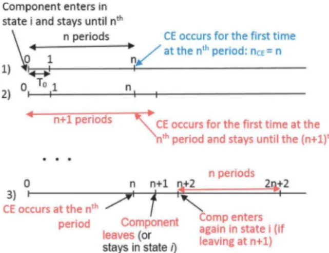
periods of T0, seeFig. 1(1):

pðnCE¼ nÞ ¼ PoccðiÞ * pnii; ð3Þ

where Pocc(i) is the occurrence probability of state i at the initial

instant. In this case, QCEðnÞ ¼ pðnCE¼ nÞ

+

period is given by the difference between:

1. the probability that CE is available at (nþ1)-th period, noted QCEðn þ 1Þ;

2. the probability that CE occurs for the first time at the n-th period and lasts until the (nþ 1)-th period, i.e. the compo-nent enters in state i at the initial period and stays in this state until (nþ1)-th period, cf.Fig. 1(2):

pðnCE¼ n þ 1Þ ¼ QCEðn þ 1Þ ' pðnCE¼ nÞ * pii

where QCEðn þ 1Þ ¼ Pocc$ Pto_i* pnii

+

at the m-th period, (nþ 1 rm o 2nþ 2) is given by pðnCE¼ mÞ ¼ QCEðmÞ ' ∑

m ' 1

a ¼ n

pðnCE¼ aÞ * pm ' aii ð4Þ

+

disappears at the (nþ1)-th period, and finally occurs again

at the ð2nþ 2Þ-th period, see Fig. 1(3). Therefore, the

prob-ability that CE occurs for the first time at the ð2nþ2Þ-th period is given by pðnCE¼ 2n þ 2Þ ¼ QCEð2n þ 2Þ ' ∑ 2n þ 1 a ¼ n þ 1 D1ðaÞ ' D2ðaÞ where

– D1ðaÞ: the probability that CE occurs for the first time at the a-th period (n þ 1 r a r 2n þ 1) and lasts until the m-th period, m ¼ 2nþ 2 in this case:

D1ðaÞ ¼ pðnCE¼ aÞ * pð2n þ 2 ' aÞii ð5Þ

– D2ðaÞ: the probability that CE occurs first time at the a-th period (nr ar m ' n' 2) and also is available at the m-th period. At m ¼ 2n þ 2, we have a¼ n; the component can stay in state i from initial period until the ð2nþ 2Þ-th period; or it leaves the state i at nþ 1 and enters again in state i at n þ 2 until the ð2nþ 2Þ-th period:

D2ða ¼ nÞ ¼ pðnCE¼ nÞ $ Pfrom_i$ Pto_i* pnii

with Pfrom_i, the row vector of size 1 $ jSj, that represents

transition probabilities from state i to all states of the state

space:

Pfrom_i¼ ½ pi1 pi2 … pii … pis.

+

at the m period (m Z 2n þ 2) is given by

pðnCE¼ mÞ ¼ QCEðmÞ ' ∑ m ' 1 a ¼ m ' n ' 1 D1ðaÞ ' ∑ m ' n ' 2 a ¼ n D2ðaÞ ð6Þ

where D1ðaÞ is calculated by Eq.(5)and

D2ðaÞ ¼ pðnCE¼ aÞ $ Pfrom_i$ Pðm ' a ' n ' 2Þtrans $ Pto_i* pnii ð7Þ

When m-1, it takes many time for evaluating D2ðaÞ (8n : nr a r m ' n ' 2) while values of D2ðaÞ can be considered as same for a Z N where N is a large number of transition steps. Therefore, in order to reduce the iterative steps, we firstly identify N such as PNtransC PN þ 1trans. Then we use N for an approximate evaluation of the

pdf of the CE. The algorithms for identifying N and for the

approximate evaluation of pðnCEÞ, 0 r nCErnmiss are presented in

the Appendix (nmissis the last period of the mission time).

When CE occurs, the system enters in the critical state until the ‘Leaving critical state’ event that occurs as soon as the component

leaves the state i. Let pðnlCE¼ mÞ be the probability that the

component leaves state i after m periods. We have

pðnlCE¼ mÞ ¼ pm ' 1ii * ð1 ' piiÞ ð8Þ

It is equal to the probability that the component stays in this state during nlCE' 1 periods and then leaves it at the ðnlCEÞ-th period.

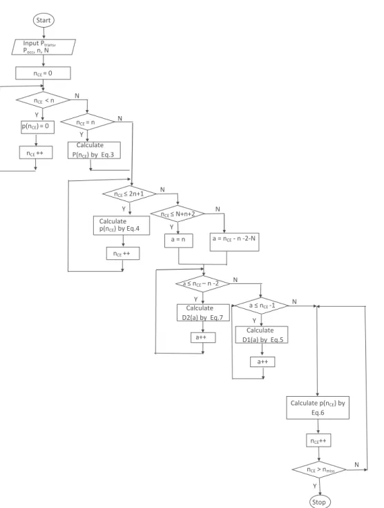
3.2. Algorithm to sample the critical events

In this subsection, we present how to directly generate the time of occurrence of the critical events (CE) for MC simulation. The first occurrence time of CE is at the m-th period, and the values of m follow the discrete function based on the approach presented in the previous subsection:

8 m o n : pðnCE¼ mÞ ¼ 0; m ¼ n : pðnCE¼ mÞ ¼ PoccðiÞ * pnii; n o m r 2n þ 1 : pðnCE¼ mÞ ¼ QCEðmÞ ' ∑ m ' 1 a ¼ n pðnCE¼ aÞ * pm ' aii 8 m Z 2n þ 2 : pðnCE¼ mÞ ¼ QCEðmÞ ' ∑ m ' 1 a ¼ m ' n ' 1 pðnCE¼ aÞ * pðm ' aÞii ' ∑ m ' n ' 2 a ¼ n

pðnCE¼ aÞ $ Pfrom_i$ Pðm ' a ' n ' 2Þtrans $ Pto_i* pnii

Ref.[17]presents a sampling approach of a discrete

distribu-tion. Let

ξ

nCEis the one that satisfies the following relation:

∑ m ' 1 j ¼ 0 pðnCE¼ jÞ o

ξ

Let PðnCErmÞ be the cumulative distribution function (cdf) of nCE,

we have

PðnCErmÞ ¼ ∑

m

j ¼ 0

pðnCE¼ jÞ: ð10Þ

Therefore, the algorithm to sample the value m of nCEfor the MC

simulation is presented inFig. 10in the Appendix. Note that we

use the modified binary search algorithm (with ‘first’, ‘last’, ‘middle’ being the integer variables) to find the sampling value m of nCEthat satisfy the Eq.(9).

3.3. Validation of the new evaluation process with a theoretical eFT In this section, we consider a theoretical example for validating and showing the efficiency of our new evaluation process for the eFT.

3.3.1. Presentation of the theoretical case and of its 3 different evaluation processes

Let us consider a sensor system that has a multi-state compo-nent A and compocompo-nent B whose time to failure follows an

exponential distribution with a failure rate of

α

component A having the probability vector of initial states, Pocc¼ ½1 0 0. and the following transition matrix every T0¼ 1 s:

Ptrans¼ 0:8 0:1 0:1 0:2 0:5 0:3 0:1 0:3 0:6 2 6 4 3 7 5

The output of the component A will be observed every T0s, and

then associated with the output of component B. The system service will be considered as failed when:

1. A is in the state 2, and B is in the failed state for more than 10 periods.

2. A is in the state 3 for more than 15 periods.

In other words, for analysing system failure, two following critical events (CE) are examined:

+

+

On the other hand, the reparation of component B is not con-sidered in this example. This assumption allows the simplification of the problem and the analytic analysis to be performed in order to compare its result with the results of several simulation approaches. In detail, the eFT of this example, presented in

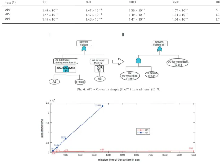
Fig. 4(I), will be quantitatively analysed using the 3 following different processes:

1. AP1 – Classical evaluation process: Convert the eFT into PN with the classical modelling approach for the component A as explained in Section 2.2.

2. AP2 – New evaluation process: Convert the eFT into PN with

the new modelling approach (presented inSections 3.1and3.2)

for the critical events (CE1, CE2) of the component A.

3. AP3 – Analytic approach: Convert the eFT into a traditional FT,

following the method presented by[22].

After evaluating the pdf, the CE is considered as a basic event. A simple eFT can be easily converted into FT, cf.Fig. 4(II). By comparing these evaluation processes, the performance of our

process (AP2) for evaluating the eFT will be highlighted inSection

3.3.3, but firstly in nextSection 3.3.2, our new modelling approach for the CE(s) considered in this eFT will be verified.

3.3.2. Validation of the new modelling approach for the critical event considered in the theoretical eFT

In order to prove the accuracy of our new modelling approach for CE, we propose to use two following ways:

W1: Model the transition process of component A by a classical PN

approach (cf. the PN structure ofFig. 11in the Appendix) in

order to evaluate the cumulative distribution function (cdf) of CE1 and CE2; then compare these results with the formula

results (Eqs. (3)–(7)) obtained when using the approximate

evaluation algorithm (cf.Fig. 9in the Appendix).

W2: Model directly the critical events CE1, CE2 using the sampling

method presented inSection 3.2in order to evaluate QCE1ðtÞ

and QCE2ðtÞ (cf. the PN structure ofFig. 12) in the Appendix;

then compare these simulation results with the theoretical results of Eq.(1).

Note that the notation of PN modelling is taken from the IEC 62551 standard[8].

These PN models are executed based on the MC simulation that are performed on the computer Core 2 Duo P8400 @2.26 GHz,

3.45 Go RAM, using the Petri net module of GRIF platform [9].

This module allows declaring new special law proposed in

Sections 3.1 and 3.2for triggering the CE transition.

The results of W1 are presented in Fig. 2. The cumulative

probabilities of CE1 (CE2) during 3600 periods obtained by both

approaches are the same. Moreover, the time to evaluate PCEby the

new simulation approach is only 4.2 s instead of 27 970 s for the

classical PN modelling approach with 3 $ 107_{simulation scenarios.}

The results of W2 are presented inFig. 3. The probabilities that

CE1 (CE2) occurs at the j-th period (0 rj r 360) obtained by the new simulation approach fluctuate around the theoretical results QCE1ðjÞ (QCE2ðjÞ) of Eq.(1).

3.3.3. Performance of the new evaluation process for evaluating the theoretical eFT

The probability of the service failure (the top event of the eFT) at

the end of the mission time Tmiss, obtained by these 3 evaluation

processes, is respectively presented inTable 2. We find that the results of the AP2 are better than the results of the AP1 when comparing with the analytic results (AP3). Moreover, for Tmiss¼ 10 000 s, the AP1

results cannot be obtained during 36 000 s of simulation time.Fig. 5

presents the simulation time for AP1 and AP2 (with 107_scenarios).

It highlights the performance of the new evaluation process, AP2. In fact, when comparing with the AP1, the longer the mission time is, the more efficient the simulation time is.

4. Case study: evaluation of the eFT related to a GNSS and ECS based localisation system

In this section, a case study of eFT is given for a GNSS & ECS based localisation unit developed in the European project,

GaLoROI[21], taken in order to illustrate the performance of our

new approach.

4.1. Description of the system and its error conditions

The localisation unit is based on the combination between GNSS and ECS measurements. Both the GNSS receiver and ECS respectively provide position and velocity of the train. These outputs are combined and matched on a digital track map in a fusion component to process an accurate train position in real-time. The service failure of GNSS & ECS based localisation unit can be classified into the following cases:

+

– A hardware failure of the fusion component directly causes an interruption of the output of the data fusion and map matching process modules.

– A software error during the fusion data process is revealed.

+

– Unavailable ECS and GNSS data: If there is no ECS and GNSS

data for more than T1s, the output of the fusion component

Fig. 3. Probability that critical event is available at t. Fig. 2. Cumulative probability of the critical events.

– Unavailable GNSS data: If GNSS data are missing for more

than T2s (ECS measurements are available) the confidence

interval linked to output data will increase quickly. In that case, the position is not trustworthy and considered as false (T1oT₂).

+

– At least k consecutive position errors of the GNSS receiver that are greater than x metres (PEr4x) can lead to a position error in output of the fusion component that exceeds the user tolerance limit.

– If ECS data are missing, at least l consecutive position errors

of the GNSS receiver that are greater than x metres (PEr4x)

can lead to a position error in output of the fusion compo-nent that exceeds the tolerance limit.

Note that due to the efficiency of the fusion process, the impact of position errors at the receiver output on the global position result will be reduced if there exists valid ECS data, thus k 4 l. The hardware failure rates of GNSS antenna, GNSS receiver, ECS, fusion component are respectively characterised by

α

α

α

α

4.2. eFT of the system

The failures of localisation service do not only depend on the material but also on satellite signal degradations due to the signal

propagation environment. This later poses multiple challenges for analysing and evaluating the service failure. In fact, common analysis approach cannot adequately take all perturbations affect-ing GNSS signals into account, especially local impacts of railway environments. In order to overcome this difficulty, we propose to use a Markov process to model the following states of the GNSS receiver:

1. Correctly estimated position, PErrx m.

2. Incorrectly estimated position, PEr4x m.

3. Unavailable position because of missing GNSS SIS (Signal In Space).

4. Unavailable position because of a hardware failure.

The transitions between the states 1/2/3 only occur when no material failure exists. Their probabilities are calculated from the

simulation data used in[1]. The transitions from these three states

to state 4 (hardware failure state) immediately occur when there exists at least a material failure of a component. After a reparation action, if all components are OK, the transition from state 4 to one of the three states 1/2/3 is fired.

Due to the efficiency of the fusion component, the degraded states (2/3/4) of the receiver output do not immediately cause a service failure. The critical events only occur when the condition of the sojourn time in degraded states is satisfied. Then, the critical

events, such as missing GNSS SIS for more than T1s or l consecutive

Fig. 4. AP3 – Convert a simple (I) eFT into traditional (II) FT.

Fig. 5. Simulation time for AP1 & AP2. Table 2

Probability of service failure for the first simple example.

Tmiss(s) 100 360 1000 3600 10 000 AP1 1:48 $ 10' 4 _{1:47 $ 10}' 4 _{1:39 $ 10}' 4 _{1:57 $ 10}' 4 _X AP2 _{1:47 $ 10}' 4 1:47 $ 10' 4 1:49 $ 10' 4 1:54 $ 10' 4 1:72 $ 10' 4 AP3 _{1:45 $ 10}' 4 1:46 $ 10' 4 1:47 $ 10' 4 1:54 $ 10' 4 1:7 $ 10' 4

(PEr4x), are modelled using the approach proposed inSection 3 (cf.Fig. 13presents the PN model of these critical events). Then, these critical events can be considered as the basic events of the eFT. The eFT of the GNSS & ECS based localisation unit is presented inFig. 6. Its notations are explained inTable 3.

The unavailable output (Case A) is caused by a material failure (Basic Event 1 – BE1) or by a software error in the fusion component (Undeveloped Event – UE). The material failure occurs with a

failure rate

α

framework of this paper.

The untrustworthy position (Case B) can be caused by a lack of

both GNSS and ECS data for more than T1s (called Intermediate

Event 1 – IE1) or by missing GNSS data for more than T2s

(Intermediate Event 2 – IE2).

Next, the IE1 can be caused by a hardware failure of ECS and

GNSS sensors for more than T1s (IE3) or missing GNSS SIS for more

than T1s when ECS fails (IE5). The IE3 is the output of a causal AND

gate (defined in[15]) with a duration greater than T1s. The output

of the causal AND gate only happens when its inputs occur together during the given period of time. This causal AND gate

Table 3

Notations of the extended Fault Tree.

Basic event: Event using a primary event failure model

Undeveloped Event: Event that is yet to be developed (not used in the following fault trees) Description Symbol: Text describing the logical result of the gate event

TRANSFER Gate: The output is used as part of a lower level tree presented in the following part REFERENCE Gate: The output is part of an upper level tree presented in the following part OR Gate: Output events occurs if any one of the input events occur

AND Gate: Output events occurs if all of the input events occur

CAUSAL AND Gate: Output events only happens when its inputs occur together during the given period of time

The DUR Gate: Output events only happens when its inputs occur during a given period of time. Fig. 6. eFT of GNSS & ECS based localisation unit.

has in input the ECS failure (Basic Event 2 – BE2) and GNSS hardware failure due to antenna failure or receiver failure (IE4).

The IE5 is the output of the AND gate having in input the DUR gate for more than T1 s of BE2 and the missing GNSS signal in space (SIS) for more than T1 s (BE3). The DUR gate is defined by the

occurrence duration of the input during a given period of time[13].

Similarly, the IE2 is caused by a duration gate for more than T2s of IE4 or the critical event, missing GNSS SIS for more than T2 s (BE4).

The case C is caused by BE5 – at least k consecutive (PEr4x m)

or IE6 – at least l consecutive (PEr4x m) when ECS fails. Then, the

IE6 is the AND gate output of the ECS failure for more than duration

time of l consecutive (PEr4xm) and the k consecutive (PE_r4x m).

4.3. Dependability analysis using the eFT evaluation method For this dependability analysis, the availability and the relia-bility of the system will be evaluated. The reliarelia-bility is defined as the ability of a system to perform a required function under given

conditions for a given time interval ½0; t.[23]. In this paper, it is expressed by the following probability:

RðtÞ ¼ PðT 4 tÞ ¼ 1 ' PðTE r tÞ ð11Þ

where TE is the service failure time, i.e. the first time the top event of the eFT occurs; and PðTE r tÞ is the system unreliability, i.e. the cumulative probability function of the service failure until t.

The instantaneous availability is the ability of a system to be in a state to perform required function under given conditions, at a given instant t[23]. In this paper, it is expressed as the probability

A(t)such as

AðtÞ ¼ Pðsystem is available at tÞ ¼ 1 ' PðTE ¼ tÞ ð12Þ

where PðTE ¼ tÞ is the system unavailability at instant t, i.e. the probability that the service failure (the top event of the eFT) occurs at t.

The eFT of the localisation unit, presented inFig. 6, cannot be

evaluated using the Analytic Approach (AP3) due to the complex-ity when considering the repairable events (with Mean Time To Repair (MTTR) is 1 h). Indeed, considering the IE3 that is the output of the gate causal AND T1, if the repair action is not considered, this gate can be easily converted into an AND gate with two inputs: (1) BE2 (ECS failure) before t-T1 and (2) IE4 (GNSS hardware failure) before t-T1. Contrarily, when repairable events are taken into account, for converting the gate CAUSAL AND T1 into a normal AND gate, we have to consider: (a) ECS failure

event occurs the n-th time at TBE2where TBE2is a random time

(0o TBE2rt ' T1) for all 1 r n r1 and (b) IE4 event occurs the

m-th time at TIE4where TIE4is a random time (0 o TIE4rt ' T1) for all

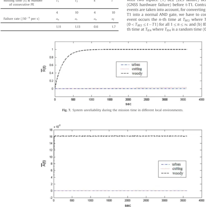
Fig. 7. System unreliability during the mission time in different local environments.

Fig. 8. System unavailability during the mission time in different local environments. Table 4

Input parameters for evaluating the failure service of system.

Missing time (s) & Number of consecutive PE

T1 T2 k l

4 10 4 10

Failure rate (/10' 9_{per s) αa αr α}

e αf

1r m r1. So, the analytical evaluation for the output of this gate

becomes complicated. On the other hand, consider T0¼ 1 s and

Tmiss¼ 3600 s, the AP1 results cannot be obtained in 20 000 s for

107_{scenarios. Therefore, the AP2 is the most appropriate approach}

for solving the eFT in order to evaluate the system dependability during 3600 s of mission time (cf.Fig. 13).

The input parameters for the system dependability analysis are

presented in Table 4. Note that these parameters are not real

parameter of the system developed in GaLoROI project. They are only used for illustrating the performance of our approach. In fact, it can take into account multi-effects of the local environments on the system dependability analysis.

The system unreliability in different local environments is

presented inFig. 7. We find that due to the masking phenomena

and the multipath effects undergone by the GNSS signals, the localisation service cannot be reliable during a long time in a woody environment.

The system unavailability in different local environments is

presented inFig. 8. At the end of the mission time, t¼3600 s, the

system unavailability can be negligible when considering a service

realised in the urban environment (PðTE ¼ 3600Þ ¼ 7:62 $ 10' 6_{) or}

in the railway cutting environment (PðTE ¼ 3600Þ ¼ 2:15 $ 10' 5_).

In the woody environment, the system unavailability can be

acceptable (PðTE ¼ 3600Þ ¼ 1:61 $ 10' 2_{) but should be improved}

by a redundancy sensor channel.

Based on the above case study, we find that the new evaluation approach is powerful to analyse the dependability of a complex system such as a GNSS-based localisation unit.

5. Conclusion

In this work, an extended Fault Tree (eFT) was proposed for qualitative analysis of complex, multi-component systems in order to identify and then to present the causes that lead to a system failure. In detail, it permits to consider the repairable multi-state components and to take into account the dependencies due to the sequences and the duration of the causes that lead to critical consequences.

For quantitative analysis, e.g evaluating the RAMS parameters, a survey of methods for evaluating the extended version of FT in literature was discussed. Among these methods, PN modelling is the most appropriate for evaluating eFT. However, as the simulation time of this classical PN modelling method is large (due to its time-dependent-feature), a new modelling process using PN for evaluating

the eFT was developed. This process is based on an analytical approach that allows directly the probability distribution function of the occurrence time of the critical event stemming from a duration of a particular gate to be captured. For the second step of the evaluation process, a sampling approach for modelling these critical events was then proposed, using its probability distribution function. The validation of the new evaluation process (AP2) was demon-strated by comparing its result with the one of a classical PN modelling process (AP1) and the analytical process (AP3). In detail, our method (AP2) gives better results than the AP1 when compar-ing with the AP3. Moreover, if the ratio between the mission time and the state transition period of the components is high, the use of the AP2 significantly reduces the simulation time.

After having enough evidences for the performance of the AP2, we then used it for the case study that cannot be solved by the AP1

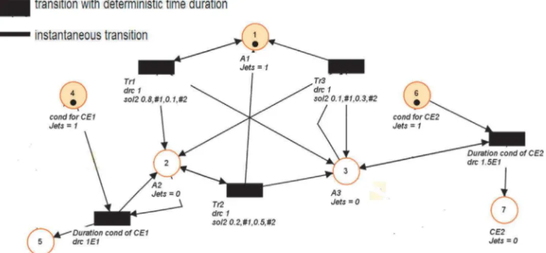
Fig. 11. PN structure for modelling the critical events of component A. Note that “sol2” in the label of Tr1, Tr2, Tr3 represents the firing law for the transitions that only one of the downstream places is filled after firing transition with a correspondent probability. For example, the label of Tr1 means that after 1 s, the token in place 1 will stay in this place with the probability 0.8, or will go to place 2 with the probability 0.1, or go to place 3 with the probability 0.1.

Fig. 12. New modelling method for critical events of component A. Note that Tr_CE1ðb; cÞ respectively represent the occurrences of CE1(from “OK_initial” state or from “OK_after_CE1” state or “OK_after_CE2” state). The transition time is triggered by the special law, noted “spec 1.1E1”. The core of this law is the sampling approach presented inSection 3.2that is based on the pdf of CE1 calculated inSection 3. Transition “leave_CE1” is triggered by the “spec 1E2” law that is based on the sampling approach of discrete distribution[17]. The next parameter of this transition represents the probability that the component will stay in the critical state in the next period.

or the AP3. In detail, a numerical example of dependability analysis for a real system – a ECS & GNSS based localisation unit was used to illustrate the performance of our approach. It allows multi-effects of the local environments in the system depend-ability analysis to be taken into account.

In further works, a biasing method to reinforce the occurrence probability of rare critical events will be considered in order to reduce the simulation time for a large number of scenarios. Furthermore, as soon as system tests in operational environments will be completed, we will analyse experimental data and will apply them into the eFT model for dependability assessments.

Acknowledgements

This research was conducted as part of the GaLoROI project (Galileo Localisation for Railway Operation Innovation) supported by the European commission. GaLoROI is an integrated research project within the European 7th Framework Programme.

Appendix

Algorithm 1 – Identify N such as PN _{converges to a rank-one}

matrix Step 1: N¼1

Step 2: Pdif¼ PðN þ 1Þtrans ' P N trans

Step 3: Let Pdifða; bÞ be the absolute value of the element at row

a-th and column b-th of the matrix Pdif.

If ∑m

a ¼ 1∑mb ¼ 1jPdifða; bÞj r10' 15, then STOP.

If NOT, N ¼ N þ 1 and returns to Step 2.

References

[1]Beugin J, Marais J. Simulation-based evaluation of dependability and safety properties of satellite technologies for railway localization. Transp Res Part C 2012;22:42–57.

[2] Bobbio A, Raiteri DC. Parametric fault trees with dynamic gates and repair boxes. In: Proceedings of reliability and maintainability, 2004 annual sympo-sium – RAMS, 2004. p. 459–65.

[3] Boudali H, Crouzen P, Stoelinga M. Dynamic Fault Tree analysis using Input/ Output Interactive Markov Chains. In: 37th Annual IEEE/IFIP international conference on dependable systems and networks, DSN 2007, Edinburgh, UK, 2007.

[4] Buchaker K. Modeling with extended fault trees. In: Fifth IEEE international symposium on high assurance systems engineering (HASE), 2000. p. 238–46. [5] Dugan JB, Salvator JB, Boyd MA. Fault trees and sequence dependencies. In:

Annual reliability and maintainability symposium, 1990. p. 286–93. [6] Fault Tree Handbook. U.S. Nuclear Regulatory Commission. Washington, DC,

1981, NUREG-0492.

[7] Filip A, Bazant L, Mocek H, Cach J. GPS/GNSS based train position locator for railway signalling. Computers in railways VII, 2000, ISBN 1-85312-826-0. [8] IEC 62551 2012. Analysis techniques for dependability-Petri Net techniques.

Standard of the International Electrotechnical Commission.

[9] GRIF, GRaphical Interface for reliability Forecasting. 〈http://grif-workshop. com/grif/petri-module/〉.

[10] Gulati R, Dugan JB. A modular approach for analyzing static and dynamic fault trees. In: Annual reliability and maintainability symposium, 1997. p. 57–63. [11]Janan X. On multistate system analysis. IEEE Trans Reliab 1985;R-34

(4):329–37.

[12]Kai Y. Multistate fault-tree analysis. J Reliab Eng Syst Saf 1990;28(1):1–7. [13] Kaiser B, Gramlich C. State-event-fault-trees – a safety analysis model for

software controlled systems. In: Proceedings of the 23rd international con-ference on computer safety, reliability, and security, SAFECOMP, 2004. p. 195– 204.

[14]Lindhe A, Norberg T, Rosén L. Approximate dynamic fault tree calculations for modelling water supply risks. Reliab Eng Syst Saf 2012;106:61–71. [15]Magott J, Skrobanek P. Timing analysis of safety properties using fault trees

with time dependencies and timed state-charts. Reliab Eng Syst Saf 2012;97:14–26.

[16]Malhotra M, Trivedi KS. Dependability modeling using petri-nets. IEEE Trans Reliab 1995;44(3):428–39.

[17] Marseguerra M, Zio E. Basics of the Monte Carlo method with application to system reliability. Hagen, Germany: LiLoLe-Verlag GmbH (Publ. Co. Ltd); 2002, ISBN 3-934447-06-6.

[18]Merle G, Roussel JM, Lesage JJ. Algebraic determination of the structure function of Dynamic Fault Trees. Reliab Eng Syst Saf 2011;96:267–77. [19] Meshkat L, Dugan JB, Andrews JD. Dependability analysis of systems with

on-demand and active failure modes using dynamic fault trees. Proc IEEE 2002; 77 (4);240–51.

[20]Murata T. Petri nets: properties, analysis and applications. IEEE Trans Reliab 2002;51(2):541–80.

[21] Nguyen K, Beugin J, Marais J. Dependability evaluation of a GNSS and ECS based localisation unit for railway vehicles. In: 13th international conference on ITS telecommunications, 2013. p. 471–6.

[22]Palshikar GK. Temporal fault trees. Inf Softw Technol 2002;44(3):137–50. [23] Railway Applications: the specification and demonstration of Reliability,

Availability, Maintainability and Safety (RAMS), project standard pr EN50126, Parts 1 to 5, CENELEC European standard – European Committee for Electrotechnical Standardization, Brussels, Belgium, 2012.

[24]Qiu S, Sallak M, Schon W, Cherfi-Boulanger Z. Modeling of ERTMS Level 2 as an SoS and evaluation of its dependability parameters using statecharts. IEEE Syst J 2014;99:1–13.

[25]Rahman FA, Varuttamaseni A, Kintner-Meyer M, Lee JC. Application of fault tree analysis for customer reliability assessment of a distribution power system. Reliab Eng Syst Saf 2013;111:76–85.

[26]Rao KD, Gopika V, Sanyasi Rao VVS, Kushwaha HS, Verma AK, Srividya A. Dynamic Fault Tree Analysis using Monte Carlo simulation in probabilistic. Reliab Eng Syst Saf 2009;94:872–83.

[27] Ross SM. Introduction to probability model. Academic Press; published December 2009, USA, ISBN: 978-0-12-375686-3.