Expansion planning of distribution networks by heuristic algorithms.

To cite this version :

Dumbrava, Virgil and Ulmeanu, Paul and Duquenne,

Philippe

and Lazaroiu, Cristian and Scutariu, Mircea Expansion planning

of distribution networks by heuristic algorithms. (2010) In: Universities

Power Engineering Conference, 31 August 2010 - 3 September 2010

(Cardiff, United Kingdom).

O

pen

A

rchive

T

OULOUSE

A

rchive

O

uverte (

OATAO

)

OATAO is an open access repository that collects the work of Toulouse researchers and

makes it freely available over the web where possible.

This is an author-deposited version published in :

http://oatao.univ-toulouse.fr/

Eprints ID : 19881

The contribution was presented at UPEC 2010 :

https://ieeexplore.ieee.org/document/5649474/references

To link to this article

URL:

https://ieeexplore.ieee.org/xpl/mostRecentIssue.jsp?punumber=5637220

Any correspondence concerning this service should be sent to the repository

administrator:

staff-oatao@listes-diff.inp-toulouse.fr

Expansion Planning of Distribution Networks by

Heuristic Algorithms

Abstract- The existing distribution networks are growing with complexity more and more, due to the gradual increase of power demand and variation of loads. This paper describes several heuristic algorithms applied to the optimal configuration of loop distribution network. Configuration problems are too complicated and time consumed to be solved. These problems are basically large-scaled combinatorial optimization problems, because an urban distribution system is usually large in scale and contain numerous sectionalizing switches to be operated. It is, therefore, difficult to rapidly obtain an exact optimal solution on real system.

Index _{Terms-- distribution power networks, heuristic} algorithms, optimal configuration

I. INTRODUCTION

In an urban distribution network the placement and installed power of loads, as well as for the supply sources, are known. Thus, the optimal routes of the branches have to be designed.

The optimal configuration of the branches routes can be solved for different network stages:

- a network area where the branches do not exist. The placement and installed power of the loads are known. The objective is to find the optimal meshed or radial configuration of the new network. The network type (meshed or radial) is previously established using analyses that consider the load density and supply reliability.

- there is an existing network, but new branches has to be build. This branches are selected from a set of lines such that to obtain the best value of the considered objective function.

Usually, the optimal configuration of a meshed network is obtained considering the minimization of branches total length. Thus, the investment in the new branches is minimal.

The methods for the optimal configuration of meshed network consider the length of a branch between the points i and j as:

- the effective distance between points i and j, calculated using the coordinates of the points in a x0y coordinates system;

- the product between the previous calculated distance and a supra-unitary coefficient that considers the irregularities of land

- the real distance determined on known branches routes.

The major part of the meshed networks have only one power source or with branches supplied by two power sources. The optimal configuration methods are different for the two types of meshed networks.

The paper deals with heuristic algorithms developed for the optimal configuration of the meshed distribution systems.

II. PROBLEM STATEMENT

The meshed networks are characterized by the fact that each of the supplied customers can receive electrical energy from two parts. Hence, the conductors of the meshed network must have constant section [1].

For the networks with unique power source, if the loads and power source placements are known, a route must be determined. This route, starting from the bus-bars, has to cross one time at each load and return to the source. In this case, the route fulfils the condition to have minim length. The loads and the power source are considered as nodes of an unordered graph. Any two nodes are connected through an edge, the needed route corresponding to one of the (n-1)! possible loops that can be made between the graph nodes, n being the total number of graph nodes. In addition, a cost of the branch can be associated to each edge. The problem obtained has a mathematical model similar with the salesman problem [2].

For a meshed network with lines fed by two sources, a mesh between two different power buses is made. In this way, the reliability of customer supply is increased.

The placement of the loads and power sources are known. The routes of the lines that connect the power sources crossing through the load buses, such that no load is not supplied and the total length of the routes has to be minimal. This problem is a combinatory optimization problem. This problem has been investigate through heuristic methods 93,4, 5], genetic algorithms [6] and expert systems [7, 8].

The solution of this problem is obtained using two heuristic algorithms, MNB and MNB – 1, each of them with one variant.

III. MATHEMATICAL MODELS

The not oriented connected graph G(V, E) defined by the set of vortices V and the set of edges E, is considered. Considering V' =

{

v_i|i=1,...,n

}

the set of vortices associated Virgil Dumbrava University POLITEHNICA of Bucharest, Romania v_dumbrava@yahoo.com Paul Ulmeanu University POLITEHNICA of Bucharest, Romania paul.ulmeanu @energ.pub.ro Philippe Duquenne Institut National Polytechnique

de Toulouse, France philippe.duquenne@ensiacet.fr Cristian Lazaroiu University POLITEHNICA of Bucharest, Romania clazaroiu@yahoo.com Mircea Scutariu Mott MacDonald Ltd, Glasgow, Scotland Mircea.Scutariu @mottmac.com

to the customers and v0 the vortex associated to the power

source, we obtainV= V' ∪

{ }

v₀ .

We consider the degree of a vortex of the graph as the number of edges incident in this node. Let lij be the length of

the edge between the vortices vi and vj. The mathematical

model, with the objective function (1) and the constraints (2) - (5) will be:

[

]

¦ ¦

n i n i j ij ijx l f 0 = =+1 = MIN (1) , ... 1, = , 1 0 n j x n j i i ij =

¦

< = (2) n 0,..., = p , 2 x x n p j 0 j pj n p < i=0 i ip +

¦

=

¦

> = (3) R, , , 1 , 1 ≤ ≠ ≤ ∈ − ≤ + − _{j ij i j} i u nx n i j n u u u (4) ° ¯ ° ® ­ = not if 0, , node after y immediatel visited, is node if 1 i j , x_ij (5)

The restriction (2) verifies the fact that each load node is visited only one time. The constraint (3) sets that each graph node has a degree of 2 (3 edges incident in each node), and the constraint (4) avoids the appearance of loops that do not cross through the source node or have less than n+1 vortices.

The solution of this problem can be obtained using heuristic methods, artificial intelligence techniques and optimization methods [9 – 13].

In [14] and [15] the “greedy” heuristic algorithm, which solves the salesman problem in a polynomial interval, is proposed. Thus, if (v0,v1,...,vk) is the link already created, then:

- if{v0,v1,...,vk} = V, then the edge (vk,v0) is added and the construction of the cycle is finished;

- if {v0,v1,...,vk} ≠ V, then the edge (vk,vk+1) with

minimum cost is added and for which vk+1∉

{v0,v1,...,vk}.

This heuristic algorithm fulfils the necessary condition to obtain a cycle starting from the vortex v0, crossing only one

time through each of the other vortices and returning then in

the vortex v0. A compromise is made: instead minimizing the

cost of the cycle, at each step the minimum cost edge is chosen.

For the incomplete graphs (there are pairs of vortices not connected through edges, due to natural field barriers), the algorithm can be applied setting to the inexistent edges cost values much greater than the costs of the existing edges. Afore presented algorithm can be applied for finding the meshed route of minimum length under the assumption that the source is balancing the demand.

Reference [16] presents an application for setting the optimum routes for new branches for connecting to the existing meshed network 6 customers and an additional source. The final network will be meshed and has a minimum length. The solution is obtained using the solving method of the salesman problem described in [17]

The mathematical model (6) – (10) can be applied for obtaining a meshed network with the form of a “moon flower”. The mathematical model is similar with the salesman problem [18].Thus, considering the source in the vortex v0,

the determination of m distinct loops of minimum length is needed. Each vortex associated to the loads is crossed only one time

[

MIN

]

f= l x n 0 = i n 1 + i = j m 1 = k ijk ij

¦ ¦ ¦

¸¸_¹ · ¨ ¨ © § (6) n 1,..., = j , 1 x n j i 0 i m 1 k ijk =

¦¦

< = = (7) m 1,..., = k ; n 0,..., = p , 2 x x n p j0 j pjk n p < i=0 i ipk +

¦

=

¦

> = (8) R u , u , n j i 1 , 1 n x n u u _{i j} m 1 k ijk j i − +

¦

≤ − ≤ ≠ ≤ ∈ = (9) ° ¯ ° ® ­ = not. if 0, ; ex after vort y immediatel visited is vortex , loop in if 1 x_ijk i j k , (10)

Reference [19] considers in addition the assumption and notations:

- all branches in a loop have the same length;

- for each loop k = 1,.., m the conductors have the maximum capacity ak;

- the demand of each load is bi, ∀ i = 1,…, n;

- the power of the source is D.

Also, the following conditions have to be fulfilled:

-

¦

¦

= ≤ m 1 k k n 1 = i i a

b í the total transmission capacity of the conductors in the m loops is at least equal with the total demand; - b D n 1 = i i≤

¦

í the source available power is at least equal with the total demand.

Considering the above presented assumptions and conditions, to the mathematical model (6) – (10) the constraint (11) can be added. Through this constraint the transmission capacity of the conductors in each loop is not exceeded.

m 1,..., = k , a x b _k n 1 = i n 0 j ijk i ¸¸≤ ¹ · ¨ ¨ © §

¦ ¦

= (11)

The different salesman problems presented in [20] and the results obtained in [21 – 26] contribute to the elaboration of mathematical models that include:

- the constraint of the loop length to a threshold value; - the constraint of the number of customers placed along

the loop such that the total demand does not exceed a threshold value;

- the determination of the optimum placement of the power source.

IV. ALGORITHMS FOR OPTIMAL CONFIGURATION OF MESHED NETWORKS SUPPLIED BY MULTIPLE SOURCES

Reference [27] proposes the MNB algorithm (Meshed Network Building) for the meshed network determination. The algorithm firstly establishes a tree scheme with minimal length of the investigated network. This scheme corresponds to the partial graph determined based on Prim algorithm [28]. From this scheme is obtained a meshed scheme through the use of minimum length branches. These braches makes possible the connection between terminal vortices connected at different power sources.

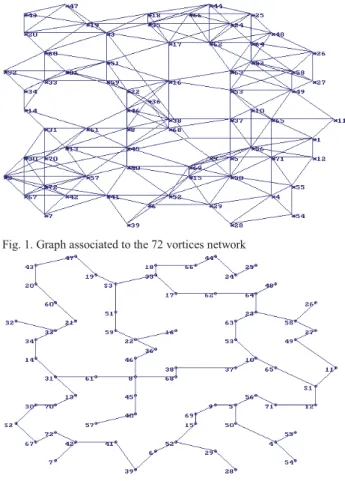
The algorithm has been tested on a distribution network with 3 sources and 69 loads [29]. The branches longer than 4 km were not considered. Under this assumption, from the 2556 possible connection between the 72 vortices, only 246 were considered. Fig. 1 shows the 246 possible branches.

Fig. 2 shows the meshed network obtained applying the MNB algorithm. Some loads will be supplied in a radial configuration.

A. Algorithm MNB – V

The heuristic algorithm MNB allows the determination of the branches routes in a meshed network with branches supplied at both terminals. The algorithm has been modified to eliminate the possibility to supply customers in a radial configuration. Applying the new algorithm, MNB – V, a complete meshed network is obtained.

The first improvement deals with the terminal vortices of the final meshed network. Each of the terminal vortices is connected through possible edges (with length smaller than the 4km threshold) to the closest vortex, which can be a terminal vortex of not.

Fig. 1. Graph associated to the 72 vortices network

Fig.2. MNB final meshed network

In this stage, the connection of more terminal vortices with one vortex (terminal or not) is not forbidden.

The second improvement modifies the edges between two vortices with a degree larger than 3 (if one vortex has a degree lower than 3, edge’s elimination will lead to the reappearance of a terminal vortex and thus of a customer radial supplied).

Fig. 3 shows the improved meshed network. No customer is supplied through radial branches. These radial branches increase the total length of the network.

With respect to the network in Fig. 2, now there 4 more branches. Hence, the meshed network MNB – V has 79 branches.

B. Algorithm MNB – 1

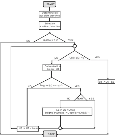
The algorithm repeatedly eliminates the edge with maximum length that is incident in vortices with a degree of at least 3. The edges selected must fulfil the condition that, after their elimination, the vortices where the edges are incident remain connected with at least two different sources. In this way is avoided the configuration illustrated in Fig. 4, where some customers can be included in a loop radial supplied.

Fig. 3. Meshed network MNB – V

At limit, if in the meshed network each vortex (power source or load) will have a degree of 2, the network will be one loop along which the power sources and the loads will be placed.

Hence, for ensuring the existence of at least this solution, the construction of a Hamiltonian cycle within the investigated graph can be achieved. The Hamiltonian cycle crosses one time in each vortex of the graph. This cycle does not have to be of minimum length [8]. References [8, 28, 30] reports the sufficient conditions such that in a graph exists a Hamiltonian cycle; the necessary conditions are not existing. In these conditions, within the MNB – 1 algorithm the constraint that each vortex of the graph must have a degree ≥ 2 is imposed.

With this constraint, at each vortex at least two edges are incident. Still, in specified situations, this constraint is not sufficient for the existance of a cycle within a graph. Fig. 5 shows a graph where each vortex has a degree of at least 2, but where no Hamiltonian cycle can be constructed.

Test network S

Branches that must not be eliminated S - Source vortex

Fig. 4. Loop that can be possibly radial supplied

Fig. 5. Graph where no Hamiltonian cycle can be constructed

The steps of the MNB – 1 are:

Step1: In a Cartesian system x0y the placements of power sources and loads are presented. All the placements will define the vortices set V.

Step 2. The distances between each two placements are calculated;

Step 3: The edges with length smaller than the threshold are retained. The edges will define the set LR;

Step 4: The condition grad(vi) ≥ 2, ∀ vi∈V is evaluated. If

the condition is not fulfilled, the algorithm stops;

Step 5: Two sets, LD and LE, are defined. The set LD contains the available branches. The set LR contains the eliminated branches. Initially, LD = LR and LE = ∅};

Step 6: As long as LD ≠ {∅}, are executed the operations: Step 6.1. The branch with maximum length is determined Lmax∈LD;

Step 6.2: The incidence of Lmax at vortices with degree at least 3 is verified. If not, Lmax is declared unavailable, is excluded from LD and the algorithm returns to Step 6.1;

Step 6.3: The construction, after eliminating Lmax, of a loop radial supplied (LRS) is verified. If not, the algorithm goes to Step 6.4. If yes, Lmax is declared unavailable, is excluded from LD and the algorithm returns to Step 6.1;

Step 6.4: the branch Lmax, which is included in LE and excluded from LD, is eliminated. The degree of the vortex where Lmax is incident is decreased with 1;

Step 7: The set LB of the branches that forms the meshed network is determined, LB = LR – LE.

The flowchart of the MNB – 1 algorithm is shown in Fig. 6.

STA RT Det erm inat ion pos s ible branc hes

Degree [v ] ≥ 2

Card (LD ) = 0 Det erm inat ion

Lm ax ∈ LD

Degree [v (Lmax )] ≥ 3

LD := LD - Lm ax

LE := LE + Lm ax D egree [v (Lmax )] : = D egree [ v (Lm ax)] -1

S TOP YE S YE S YE S NO NO NO B A R Y E S NO LB : = LR - LE Sel ect ion

admi tt ed branches

Fig. 7 illustrates the meshed network determined applying the MNB – 1 algorithm, using same inputs as for the MNB.

The maximum admissible length of the branches is smaller than 3.25. The constraint that each vortex of the initial graph must have a degree at least of 2 is not fulfilled, thus there are customers radial supplied.

This results is not a drawback of the used method, but is determined by the physical inexistence of some branches incident in the respective vortices.

C. Algorithm MNB – 1V

In this algorithm an additional constraint has been introduced. The elimination of the branches incident at the source vortices is forbidden until the construction of the meshed network is finished.

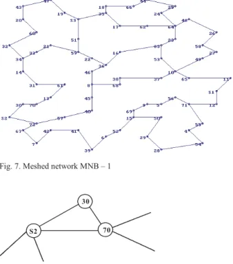
In this way, the number of outputs from each power source increases, which leads to an increase of reliability supply of the customers. If local loops containing power source vortices are composed, in a later step the edges incident in vortices with degree ≥ 3 are eliminated. In Fig. 8 a local loop determined by the vortices S2, 30 and 70 is illustrated. The edge S2-70 can be eliminated without the risk for appearing customers radial supplied.

Fig. 9 shows the meshed network obtained applying the MNB – 1V algorithm, using the same input data.

V. APPLYING THE ALGORITHM TO THE EXISTING NETWORKS

The methods presented for the determination of new meshed networks can be also applied for studying the development of the existing networks.

The placements of all new and existing power sources, as well as of all new and existing customers, are known.

Fig. 7. Meshed network MNB – 1

S2

30

70

Fig. 8. Local loop

Fig. 9. Meshed network MNB – 1V

In first, all new possible branches that can be established is in network are calculated. From these new branches, the ones that cannot be realized due to natural obstacles or environmental barriers are eliminated. The branches already existing are considered of length zero.

Any of the previously presented algorithms can be applied, in two cases:

- none of the old branches is eliminated, even if determine additional not essential loops;

- the elimination of the old branches, for obtaining a final meshed network with smaller total length, is allowed.

In addition, the problem of meshed network with total length minimum can be transformed in the problem of meshed network with minimum costs. Thus, the length lij of

the new branch between the vortices i and j can be replaced in the problem with the product lij⋅kij, where kij is the average

cost for conductor pulling per unit of length, between the vortices i and j.

In this way, the different costs for realizing two different routes with same length, but in different environmental conditions, can be considered.

In addition, studies regarding the influence of placement, or sources number, modification on network configuration can be conducted.

VI. CONCLUSIONS

Table I reports the total lengths for the looped networks obtained with the four methods for the same set of data (coordinates of sources and consumers). It is also presented the value of minimum active power losses for the un-looped operation diagram of each network.

The un-looped operation diagrams were determined using the SURF algorithm, which is presented in [19], whilst the entry data required were taken from [29].

Analyzing the results repoted in Table I it is noted that the smallest value of active power losses for un-looped operating diagrams corresponds to the network with the highest value of total length of lines, with the largest number of branches and with the greatest number of loops.

TABLE I RESULTS Algorithm Total length [km] Active losses [kW] Number of branches Number of loops MNB 144.203 202.867 75 4 MNB-V 158.430 194.386 79 8 MNB-1 157.897 195.900 79 8 MNB-1V 167.705 135.932 80 9

It follows that establishing a network configuration must not be done according only to the total length of branches, namely the minimum cost of electric conductors. We must consider also the value of network losses as a component of operating expenses.

The looped networks determined using the methods described in this paper can be also studied and in terms of consumers security of supply and damages.

Algorithms presented may be useful in the design and study of urban power distribution network development, especially when integrated into computer applications for GIS (Geographic Information System).

REFERENCES

[1] Z. Bozic, E. Hobson, “Urban underground network expansion planning,” IEE Proc. GTD, vol. 144, pp. 118 – 124, March 1997. [2] A. Russel, M. Sasieni, Basis of operational research. Bucharest :

Technical, 1975.

[3] K. Aoki, K. Nara, T. Satoh, M. Kitagawa, K. Yamanaka, “New approximate optimization method for distribution system planning,”

IEEE Trans. Power Syst., vol.5, pp.126 – 132, 1990.

[4] K. Nara, T. Satoh, H. Kuwabara, K. Aoki, M. Kitagawa, T. Ishihara, “Distribution systems expansion planning by multi-stage branch exchange,” IEEE Trans. Power Syst., vol.7, pp. 208 - 214, 1992. [5] K. Nara, H. Kuwabara, M. Kitagawa, K. Ohtaka, “Algorithm for

expansion planning in distribution systems taking faults into consideration”, IEEE Trans. Power Syst., vol. 9, pp. 324 – 330, 1994. [6] V. Miranda, J.V. Ranto, L.M. Proenca, “Genetic algorithms in

multistage distribution network planning,” IEEE Trans. Power Syst., vol. 9, pp. 1927-1933, 1994.

[7] J.L. Chen, Y.Y. Hsu, “An expert system for load allocation in distribution expansion planning,“ IEEE Trans. Power Del., vol. 4, pp. 1910 – 1918, 1989.

[8] Y.Y. Hsu, J.L. Chen, “Distribution planning using a knowledge-based expert system,” IEEE Trans. Power Del., vol. 5, pp. 1514 – 1519, 1990. [9] C.E. Miller, A.W. Tucker, R.A. Zemplin, “Integer Programming Formulation of Traveling Salesman Problems”, J. ACM, vol. 7, pp. 326-329, 1960.

[10] N. Christofides, “The Traveling Salesman Problem,” Report 77-11, December 1977, Department of Management Science, Imperial College, London SW7 2Bx.

[11] F. Marshall, Network Routing. in OR & MS, vol. 8, Elsevier Science B.V., 1995.

[12] B.E. Gillet, L.R. Miller, “A Heuristic Algorithm for the Vehicle-Dispatch Problem,” Operations Research, vol. 22, pp. 340-349, 1974. [13] G. Clarke, J.W. Wright, “Scheduling of Vehicles from a Central Depot

to a Number of Delivery Points,” Operations Research, vol. 12, pp. 568-581, 1964

[14] L. Livovschi, H. Georgescu, Synthesis and analysis of algorithms, Bucharest: Scientific, 1986.

[15] I. Odagescu, C. Copos, D. Luca, F. Furtuna, I. Speureanu, Programming methods and techniques, Bucharest: Intact, 1994. [16] A. Stanculescu, “Operational method for determining the optimal

routes in distribution systems,” Energetica, vol. 10, pp.351-357, 1978.

[17] J.D.C. Little, K.G.Murty, D.W. Sweeney, C. Karel, “An Algorithm for the Traveling Salesman Problem,” Operations Research, vol. 11, pp. 972-989, 1963.

[18] N. Christofides, A. Mingozzi, P. Toth, “Exact Algorithms for the Vehicle Routing Problem, Based on Spanning Tree and Shortest Path Relaxations,” Mathematical Programming, vol. 20, pp. 255-282, 2005 [19] V. Dumbrava, “Optimizaton of the structure and operation of

distribution systems,” PhD Thesis, University POLITEHNICA of Bucharest, 1998.

[20] G. Laporte, Y. Nobert, “Subtour elimination algorithms for the symmetrical travelling salesman problem and its variants,” Report no.80-04, Center for Researc on Transportation, Montreal, 1980. [21] F. Marshall, “Optimal Solution of Vehicle Routing Problems Using

Minimum K-Trees,” Operations Research, vol. 42, pp. 626-642, 1994. [22] P. Milliotis, “Integer Programming Approaches to the Travelling

Salesman Problem,” Mathematical Programming, vol. 10, pp. 367-378, 1976.

[23] P. Milliotis, “Using Cutting Planes to Solve the Symmetric Travelling Salesman Problem,” Mathematical Programming, vol. 15, pp. 177 – 188, 1978.

[24] M. Bellmore, J.C. Malone, “Pathology of Traveling-Salesman Subtour-Elimination Algorithms,” Operations Research, vol. 19, pp. 278 – 307, 1971.

[25] S. Lin, “Computer Solutions of the Traveling Salesman Problem,” Bell

System Tech. J., vol. 65, pp. 2245 – 2269, 1965.

[26] S. Lin, B.W. Kernighan, “An effective Heuristic Algorithm for the Traveling-Salesman Problem,” Operations Research, vol.21, pp. 498 – 516, 1973.

[27] V. Dumbrava, Th. Miclescu, G. Bazacliu, “Sequential algorithm for planning the distribution system routes,” Energetica, vol. 6, pp. 268-272, 1996

[28] S.C. Savulescu, Graphs and electrical networks, Bucharest: Technical, 1994.

[29] V. Glamocanin, V. Filipovic, “Open loop distribution system design,”

IEEE Trans. Power Del., vol.8, pp. 1900 – 1906, 1993.

[30] C. Croitoru, Basic techniques in combinatory optimization, Iasi: University, 1992