HAL Id: hal-01251244
https://hal.inria.fr/hal-01251244
Submitted on 5 Jan 2016HAL is a multi-disciplinary open access
archive for the deposit and dissemination of sci-entific research documents, whether they are pub-lished or not. The documents may come from
L’archive ouverte pluridisciplinaire HAL, est destinée au dépôt et à la diffusion de documents scientifiques de niveau recherche, publiés ou non, émanant des établissements d’enseignement et de
Approximate reflectional symmetries of fuzzy objects
with an application in model-based object recognition
Olivier Colliot, Alexander V. Tuzikov, Roberto M. Cesar, Isabelle Bloch
To cite this version:
Olivier Colliot, Alexander V. Tuzikov, Roberto M. Cesar, Isabelle Bloch. Approximate reflectional symmetries of fuzzy objects with an application in model-based object recognition. Fuzzy Sets and Systems, Elsevier, 2004, 147 (1), pp.141-163. �10.1016/j.fss.2003.07.003�. �hal-01251244�
Approximate reflectional symmetries of fuzzy
objects with an application in model-based
object recognition
Olivier Colliot
a, Alexander V. Tuzikov
b,1, Roberto M. Cesar
c,2,
Isabelle Bloch
a,2,∗
aEcole Nationale Sup´erieure des T´el´ecommunications, D´epartement TSI,
CNRS URA 820, 46 rue Barrault, 75634 Paris Cedex 13, France
b Research-Engineering Center of Informational Technologies, National Academy
of Sciences of Belarus, Akademicheskaja 25, 220072 Minsk, Belarus
cDepartment of Computer Science, Institute of Mathematics and Statistics - IME,
University of S˜ao Paulo - USP Rua do Mat˜ao, 1010, S˜ao Paulo, SP CEP 05508-090 - Brazil
Abstract
This paper is devoted to the study of reflectional symmetries of fuzzy objects. We introduce a symmetry measure which defines the degree of symmetry of an object with respect to a given plane. It is computed by measuring the similarity between the original object and its reflection. The choice of an appropriate measure of com-parison is based on the desired properties of the symmetry measure. Then, an algorithm for computing the symmetry plane of fuzzy objects is proposed. This is done using an optimization technique in the space of plane parameters. Finally, we illustrate our approach with an application where the symmetry measure is used as an attribute in graph matching for model-based object recognition.
Key words: plane symmetry, symmetry measure, measures of comparison, measures of similarity, optimization, pattern recognition
∗ Corresponding author. Tel: +33 1 45 81 75 85, Fax: +33 1 45 81 37 94 Email addresses: [email protected] (Olivier Colliot),
[email protected] (Alexander V. Tuzikov), [email protected] (Roberto M. Cesar), [email protected] (Isabelle Bloch).
1 A. Tuzikov was supported by a sabbatical grant at the Department of Signal and
Image Processing (ENST) and is very grateful to the department for its hospitality.
2 R. Cesar and I. Bloch were partially supported for this work by a CAPES /
COFECUB grant (number 369/01). R. Cesar is grateful to FAPESP (99/12765-2) and to CNPq (300722/98-2).
1 Introduction
Different kinds of symmetry (central, reflection, rotation, skew) have been widely studied in the fields of image processing and computer vision. For scene description and recognition, symmetry is an important feature. It can be an attribute of the objects themselves, a relation between two objects or it can be used to compute other relationships between objects (e.g. directional relationships [8]). This paper is devoted to the case of reflectional symmetries also called bilateral symmetries. The study is done for plane symmetries in the 3D Euclidean space but all results are also valid for axial symmetries in 2D.
Exact symmetry usually does not exist in real objects and one has to deal with approximate symmetries. Many works quantify the degree of symmetry using a symmetry measure often based on a distance. For example, Marola [18] uses the normalized l2 metric between the original and the reflected image. O’Mara
and Owens [21] use the difference between grey levels in 3D images. Minovic et al. [20] use an octree representation to define a symmetry measure corre-sponding to the size of the largest symmetrical subset of an object. Heijmans and Tuzikov [13] define symmetry measures for convex sets using Minkowski addition. Zabrodsky et al. [32] introduce a symmetry measure for shapes (i.e. sets of points) that quantify the minimum effort to turn any given shape into a symmetrical one. Their approach takes into account uncertainty by modeling point localizations as a probability distribution.
However, apart from the previous reference [32], most results have been ob-tained for precisely defined objects. We consider the case of 3D fuzzy objects (i.e. fuzzy subsets of 3D space) which have found increasing application in image processing. Following the classical approach used for crisp shapes and images, we define a symmetry measure which characterizes the degree of sym-metry of an object with respect to a given plane (Section 2). For this we use a measure of comparison3 between the object and its reflection. Various
mea-sures of comparison have been proposed in the literature for fuzzy sets. We present the properties that should be verified by the symmetry measure for its use in pattern recognition. The choice of a measure that is appropriate to our problem is based on these properties (Section 3) as discussed in [8]. In Section 4, we study the case of objects with a principal symmetry plane and propose an algorithm for symmetry plane computation. This algorithm is based on an optimization technique and uses the principal axes of inertia to define an initial position of the symmetry plane. In Section 5, we illustrate
3 We prefer to use the expression “measure of comparison” as in [5] instead of
“similarity measure”, since different authors assume different properties for the notion of similarity measure.
how symmetry measures can be used in concrete image recognition problems: the symmetry measure is used as a relation between objects in model-based pattern recognition through the definition of a graph attribute integrated in the approach proposed in [6].
2 Symmetry measure
2.1 Reflection of a fuzzy object
Let Π be a plane in the 3D spaceR3 and Ω a subset ofR3 (or Z3 in the digital
case). We denote by F the set of fuzzy subsets of Ω and for a fuzzy set A, µA
denotes its membership function. Given a point x of Ω, we denote by eΠ(x) its
image under the reflection with respect to Π. The mapping eΠ is a bijective
transformation in R3. Therefore, one can define the reflection of a fuzzy set as
follows.
Definition 2.1 The reflection of a fuzzy set A is a fuzzy set eΠ(A) defined
as:
µeΠ(A)(eΠ(x)) = µA(x) for every x∈ Ω.
We denote by eu,d the reflection with respect to a plane Πu,d which is
or-thogonal to u and passing at the signed distance d from the origin. In spher-ical coordinates a unit vector u is defined by two angles β ∈] − π, π] and α∈ [−π/2, π/2] (see Fig. 1). As vectors u and −u define the same plane, we use β ∈ [0, π[, α ∈] − π/2, π/2] and d ∈ R. α β O z u y x
Fig. 1. Angles α and β define a unit vector u
We also use notation eα,β,d instead of eu,d in 3D, and eβ,d = e0,β,d in 2D.
2.2 Symmetry measure
We want to define a symmetry degree of a fuzzy object with respect to a given plane Π. One option is to compare A and eΠ(A). A symmetry measure σA
can be defined as a measure of comparison between the original object and its reflection:
σA(Π) = S(A, eΠ(A)),
where S is a measure of comparison between fuzzy objects. As before, we use notations σA(u, d) = σA(α, β, d) = σA(Πu,d).
Various measures of comparison have been proposed in the literature. They possess different properties and the choice of a measure depends on the appli-cation and on the concept one wants to describe.
2.3 Desired properties of symmetry measures
In order to choose appropriate measures of comparison, it is useful to present which properties should be satisfied by a symmetry measure. In this section, we summarize properties of measures of comparison found in the literature and discuss which of them are useful to derive a symmetry measure.
2.3.1 Measures of similitude
Bouchon-Meunier et al. [5] have proposed a classification of measures of com-parison between fuzzy sets, in particular M-measures of comcom-parison which are derived from a fuzzy measure M .
Definition 2.2 [5] An M-measure of comparison is a mapping S :F × F → [0, 1] such that S(A, B) = FS
µ
M (A∩ B), M(B − A), M(A − B)
for a given mapping FS :R+× R+× R+ → [0, 1] and a fuzzy measure M.
A particular class of measures of comparison is composed of measures of simil-itude.
Definition 2.3 [5] An M-measure of similitude is an M-measure of compar-ison S such that FS(u, v, w) is non-decreasing in u, non-increasing in v and
w.
M-measures of similitude are well suited for describing symmetries: symmetry is stronger if the measure of intersection between the original object and its reflection increases, and it is weaker if the measure of difference between them increases.
Measures of similitude include measures of satisfiability and measures of re-semblance.
Definition 2.4 [5]
(1) An M-measure of satisfiability is an M-measure of similitude such that • FS(u, v, w) is independent of w;
• FS(0, v, w) = 0, for all v, w (exclusivity);
• FS(u, 0, w) = 1, for all u 6= 0 (inclusion).
(2) An M-measure of resemblance is an M-measure of similitude such that • S is reflexive, i.e. S(A, A) = 1.
• S is symmetrical, i.e. S(A, B) = S(B, A).
In our case, since we have M (A − eΠ(A)) = M (eΠ(A)− A), measures of
satisfiability are also measures of resemblance [5]. Moreover, the exclusivity property entails that the symmetry measure is equal to zero when the plane passes outside the support of the object (in the case of a support with only one connected component). This is considered desirable by Marola [18]. The inclusion property, as well as reflexivity, entails that the symmetry degree is equal to 1 when the object coincides with its reflection, i.e. when there is an exact symmetry. The symmetry property implies that the symmetry measure for an object A with respect to a given plane Π is equal to the measure computed for its reflection eΠ(A):
∀A, B ∈ F, S(A, B) = S(B, A) =⇒ ∀A ∈ F, S(A, eΠ(A)) = S(eΠ(A), A)
Since eΠ(eΠ(A)) = A, we have:
∀A, B ∈ F, S(A, B) = S(B, A) =⇒ ∀A ∈ F, σA(Π) = σeΠ(A)(Π)
Therefore, M-measures of satisfiability seem to be suitable for the definition of measures of symmetry.
2.3.2 Additional properties
Pappis [22] proposes the following additional properties which are in fact the reverse implications of reflexivity and exclusivity, leading to the follow-ing equivalences:
S(A, B) = 1 ⇐⇒ A = B,
S(A, B) = 0 ⇐⇒ supp(A) ∩ supp(B) = ∅.
where supp(A) is the support of A. The first property, also called separability for distances, expresses that the symmetry measure is equal to 1 if and only if there is an exact symmetry. The second one expresses that the symmetry measure equals zero if and only if the plane passes outside the support of the object. These properties are desirable for defining symmetry measures.
2.3.3 Geometrical properties
Intuitively speaking a symmetry measure should be invariant with respect to translation, rotation and scaling. If S is invariant w.r.t. translation (respec-tively rotation) then so is σ. This is also true for scaling but as the scaling of a fuzzy set in the discrete case is not clearly defined, we will not consider it later on.
2.3.4 Summary of properties
Using our properties we are now able to provide a definition of a symmetry measure satisfying our requirements:
Definition 2.5 The symmetry measure of A with respect to Π is defined as: σA(Π) = S(A, eΠ(A)),
where S is a measure of comparison with the following properties: (P1) Symmetry: S(A, B) = S(B, A);
(P2) Reflexivity: S(A, B) = 1 ⇐⇒ A = B;
(P3) S(A, B) = 0 if and only if the supports of A and B are disjoint; (P4) S is invariant w.r.t. translation;
(P5) S is invariant w.r.t. rotation.
Additionally, one can require that S is an M-measure of similitude. Properties (P1), (P2) and (P3) ensure that it will also be an M-measure of satisfiability and of resemblance.
Other properties of measures of comparison considered for instance in [5,17,22] are either equivalent to these ones or not interesting for deriving symmetry measures.
3 Deriving symmetry measures from measures of comparison
We summarize which of the previous properties hold for different measures of comparison proposed in the literature and select some of them to define symmetry measures. We use here a classification of measures of comparison that is very similar to the ones used in [34] and [4].
3.1 Set-theoretic approach
Most of the measures discussed in this section have been derived from a general measure proposed by Tversky [28] and are based on combinations of µA and
µB using t-norms and t-conorms. They satisfy (P1) as t-norms and t-conorms
are commutative. The following measure has been used by several authors [5,9,22,34] 4: S1(A, B) = P x∈Ω>(µA(x), µB(x)) P x∈Ω⊥(µA(x), µB(x))
where> is a t-norm and ⊥ is a t-conorm [9]. Property (P2) holds if and only if> = min and ⊥ = max 5. Property (P3) is fulfilled for t-norms “minimum”
and “product” but is not for “drastic” and “Lukasiewicz” ones 6 [9]. Properties
(P4) and (P5) are fulfilled.
Wang [29] proposed the following measure of comparison: S2(A, B) = 1 |Ω|× X x∈Ω >(µA(x), µB(x)) ⊥(µA(x), µB(x))
where |Ω| denotes the cardinality of Ω and with 0
0 = 1. S2 satisfies (P2) if
and only if > = min and ⊥ = max but does not satisfy (P3).
However, it is easy to check that a modified version of S2 defined as follows:
S3(A, B) = 1 |supp(A) ∪ supp(B)| × X x∈supp(A)∪supp(B) >(µA(x), µB(x)) ⊥(µA(x), µB(x))
satisfies property (P3) for t-norms “minimum” and “product”. Properties (P4) and (P5) are also fulfilled.
Hyung et al. [14] proposed to use a measure of comparison defined as S4(A, B) = max
x∈Ω >(µA(x), µB(x)).
Measure S4 satisfies property (P3) for “minimum” and “product” t-norms
but does not satisfy (P2).
4 Here we deal with the finite discrete case. In the continuous case, the sum is
replaced by an integral if it converges.
5 Proofs can be found in the appendix
6 The usual t-norms are the minimum, the product, the Lukasiewicz t-norm defined
as>(a, b) = max(0, a + b − 1) and the drastic t-norm defined as >(a, b) = b if a = 1, a if b = 1, 0 otherwise.
3.2 Lp distance approach
In this section we use the Lp distance between fuzzy sets A and B:
kA − Bkp = Ã X x∈Ω |µA(x)− µB(x)|p !1p kA − Bk∞= max x∈Ω(|µA(x)− µB(x)|).
Measures of comparison based on the Lp distance have the following general
form:
S(A, B) = 1− kA − Bkp
K ,
where K is a normalization coefficient. It is easy to see that properties (P1), (P2), (P4) and (P5) are fulfilled for measures of this type.
For example, Wang [29] and Bouchon-Meunier et al. [5] proposed the following measure
S5(A, B) = 1− kA − Bk1
|Ω| .
This measure does not satisfy property (P3). The following measure of com-parison proposed by Pappis [22]
S(A, B) = 1− P x∈Ω|µA(x)− µB(x)| P x∈Ω[µA(x) + µB(x)] can be generalized as S6(A, B) = 1− kA − Bkp (P x∈ΩµA(x)p+ µB(x)p) 1 p
Measure S6 satisfies property (P3).
Pappis [22] also proposed to use the L∞ distance
S7(A, B) = 1− kA − Bk∞
Measure S7 does not satisfy property (P3). However, when A and B are
normalized fuzzy sets and their supports are disjoint S7(A, B) = 0. But the
converse implication is still false.
It is easy to verify that the measure of comparison (β > 0) S8(A, B) = e−βkA−Bkp
Other measures exist, like for example the correlation coefficient between fuzzy sets [12], but they do not satisfy our properties.
Table 1
Summary of properties of measures of comparison. For measures S1, S2, S3, these
results are valid only for some particular t-norms and t-conorms. The symbol √ means that a property is satisfied, while× means that it is not.
Measure of comparison (P1) (P2) (P3) (P4) (P5) S1(A, B) = P x∈Ω>(µA(x),µB(x)) P x∈Ω⊥(µA(x),µB(x)) √ √ √ √ √ S2(A, B) = |Ω|1 ×P x∈Ω >(µA(x),µB(x)) ⊥(µA(x),µB(x)) √ √ × √ √ S3(A, B) = |supp(A)∪supp(B)|1 ×Px >(µA(x),µB(x)) ⊥(µA(x),µB(x)) √ √ √ √ √ S4(A, B) = maxx∈Ω>(µA(x), µB(x)) √ × √ √ √ S5(A, B) = 1−kA−Bk|Ω| 1 √ √ × √ √ S6(A, B) = 1− kA−Bkp (P x∈ΩµA(x)p+µB(x)p) 1 p √ √ √ √ √ S7(A, B) = 1− kA − Bk∞ √ √ × √ √ S8(A, B) = e−βkA−Bkp √ √ × √ √
3.3 Chosen symmetry measures
The measures of comparison S1, S3 (for t-norm “minimum”) and S6 satisfy
properties (P1)-(P5) (see Table 1).
Therefore we define three symmetry measures: σ1,A(Π) = P x∈Ωmin(µA(x), µeΠ(A)(x)) P x∈Ωmax(µA(x), µeΠ(A)(x)) σ2,A(Π) = 1
|supp(A) ∪ supp(eΠ(A))|×
X x∈supp(A)∪supp(eΠ(A)) min(µA(x), µeΠ(A)(x)) max(µA(x), µeΠ(A)(x)) σ3,A(Π) = 1− kA − e Π(A)kp ³ P x∈ΩµA(x)p+ µeΠ(A)(x) p´ 1 p .
However, S1 has the additional advantage of being an M-measure of similitude
which guarantees some good monotony properties. As we will see in the next section, it is preferable to use S1.
3.4 Study of σA on examples
Let us see, through some examples, how the value of a symmetry measure can be interpreted.
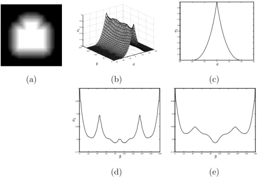
Figure 2 shows the shape of σ1,A(β, d) for a synthetic 2D fuzzy object (see
Section 2.1 for the notations). This function has four modes which correspond to four local maxima and to four axes of local symmetry: one axis of exact symmetry (β = 0o , d = 0), two axes of strong but not exact symmetry
(β = 45o or 135o, d = 0) and one axis of weak symmetry (β = 90o, d = 0) 7.
As expected, one has σA(Π) = 1 for an exact symmetry axis. We can also see
that a set A has a local symmetry plane Πα,β,d if a symmetry measure σA has
a local maximum in (α, β, d). Thus, to find the local symmetry planes of A one has to find the local maxima of σA. Figure 2 also compares the behavior of σ1,A
and σ3,A for d = 0. Although their shapes are similar, one can see a difference
in the neighborhood of β = 90o which is a local maximum for σ
1,A but a
local minimum for σ3,A. In fact, this is not surprising as we have monotony
properties only for M-measures of similitude (Def. 2.3) and therefore only for σ1,A. In other cases, the behavior cannot be predicted.
−30 −20 −10 0 10 20 30 0 50 100 150 200 0 0.2 0.4 0.6 0.8 1 d β σ1 −300 −20 −10 0 10 20 30 0.1 0.2 0.3 0.4 0.5 0.6 0.7 0.8 0.9 1 d σ1 (a) (b) (c) 0 20 40 60 80 100 120 140 160 180 0.75 0.8 0.85 0.9 0.95 1 β σ1 0 20 40 60 80 100 120 140 160 180 0.75 0.8 0.85 0.9 0.95 1 β (d) (e)
Fig. 2. (a) A 2D fuzzy set A (high grey levels correspond to high membership values). (b) σ1,A. (c) σ1,A for β = 0. (d) σ1,A for d = 0.(e) σ3,A (p = 2) for d = 0.
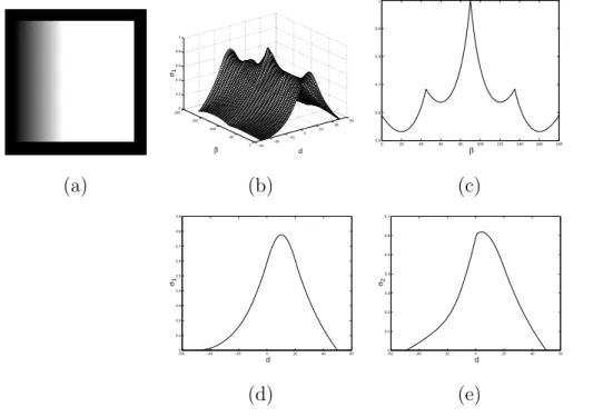
Figure 3 shows the shape of σ1,A(β, d) for another 2D fuzzy object. In the
direction defined by β = 0, the maximum of σ1,A is obtained for d = 10 which
is the position of the symmetry plane of the α-cut of level 0.5. This result fits
well with the intuition. Figure 3 also shows the shape of σ2,A. For this measure,
the maximum in the direction defined by β = 0 is obtained for d = 4. The difference between the two measures can again be explained by the fact that only σ1,A is an M-measure of similitude.
−60 −40 −20 0 20 40 60 0 50 100 150 200 0 0.2 0.4 0.6 0.8 1 d β σ1 0 20 40 60 80 100 120 140 160 180 0.5 0.6 0.7 0.8 0.9 1 β (a) (b) (c) −600 −40 −20 0 20 40 60 0.1 0.2 0.3 0.4 0.5 0.6 0.7 0.8 0.9 d σ1 −600 −40 −20 0 20 40 60 0.1 0.2 0.3 0.4 0.5 0.6 0.7 d σ2 (d) (e)
Fig. 3. (a) A 2D fuzzy set A. (b) σ1,A. (c) σ1,A for d = 0. (d) σ1,A for β = 0. (e)
σ2,A for β = 0.
The measure σ1 seems to have the best properties. In the following of the
paper, we only use this measure as a symmetry measure and we denote:
σA(Π) = P
x∈Ωmin(µA(x), µeΠ(A)(x))
P
x∈Ωmax(µA(x), µeΠ(A)(x))
4 Symmetry plane computation
In this section, we consider the case of an object with a main approximate symmetry plane i.e. a plane which corresponds to a global maximum in the symmetry measure. To find this symmetry plane, one has to find the plane for which the symmetry measure has a maximum i.e.
max
α∈]−π/2,π/2], β∈[0,π[, d∈RσA(α, β, d)
Whereas the computation of σA for a sufficiently small step is feasible in the
only wants to locate the best symmetry plane of an object corresponding to the largest symmetry measure value. We propose a method that expresses the problem of finding the best symmetry plane as an optimization problem in the parametric space ]− π/2, π/2] × [0, π[×R (Figure 4 presents an outline of the algorithm).
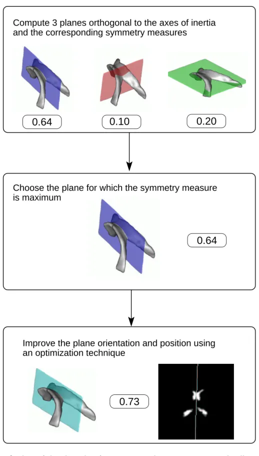
The optimization procedure needs a starting point. We suggest to use the ellipsoid of inertia to define candidates for this starting point. The ellipsoid of inertia has already been used in [21] to define the symmetry plane of an object. Here it is only taken as an initialization. The directions of axes are defined as the eigenvectors of the inertia matrix:
m200 m110 m101 m110 m020 m011 m101 m011 m002
Here mpqr defines a central moment of order p + q + r:
mpqr(A) = X
Ω
µA(x, y, z)(x− xc)p(y− yc)q(z− zc)r,
where c = (xc, yc, zc) is the center of mass of the fuzzy object. If a 3D
ob-ject possesses an exact plane of symmetry it passes through its center of mass and is orthogonal to one of the ellipsoid axes. Let us denote by u1,
u2 and u3 the eigenvectors of the inertia matrix. We consider then three
planes orthogonal to these vectors and passing through the center of mass: Π1 = Πu1,u1·c, Π2 = Πu2,u2·c and Π3 = Πu3,u3·c (where u· c denotes the inner
product). Our initial symmetry plane Πi maximizes the symmetry measure,
i.e. σA(Πi) = max{σA(Π1), σA(Π2), σA(Π3)}. This is only possible when the
eigenvectors are different. Otherwise, one gets an ellipsoid of revolution. This plane is just an initial guess, not the symmetry plane. The symmetry plane is found using an optimization technique. We use the Nelder-Mead down-hill simplex method [26] which was also used in [1] for grey-level images with a different initialization and a different symmetry measure. This method is often used when one does not know the function derivatives. It is accurate and robust under a good starting point. However, it is a local optimization method and, in general, one has no guarantee to find the global maximum. This method starts from a simplex in the parametric space. In our case, the dimension is three and the simplex is a tetrahedron. We place our initial point at one of the tetrahedron vertices and compute the 3 other points by only modifying one parameter at a time (in other words, each vertex is on an axis of the parametric space). The complete procedure for symmetry plane com-putation takes 25 seconds to achieve a precision of 10−3 for the symmetry
0.64
0.73
0.64
and the corresponding symmetry measuresCompute 3 planes orthogonal to the axes of inertia
0.20
0.10
Choose the plane for which the symmetry measure
Improve the plane orientation and position using an optimization technique
is maximum
Fig. 4. Outline of the algorithm for symmetry plane computation. The illustration is a fuzzy segmentation of lateral ventricles in a 3D MR image of the brain. We present 3D renderings of the 0.5 α-cut and a slice of the fuzzy set.
This computation time is very reasonable. If needed, it is possible to achieve a faster computation time by undersampling the objects.
5 Symmetry measure as a graph attribute for facial feature recog-nition
Model-based pattern recognition often makes use of graph representations, where vertices and edges are attributed. These attributes are used for compar-ing the image to be recognized and the model, in a graph matchcompar-ing procedure. Typically vertices represent image regions, with attributes such as grey lev-els, texture and shape measures, while edges represent relationships between regions, with attributes such as distances and relative directional position. In this section, we show how symmetry measures can be used to define edge attributes between image regions in such structural models.
The application concerns the recognition of facial features such as pupils, nos-trils and mouth based on a face model. This is an important task in face recog-nition [33] and facial expression analysis [10]. Symmetry has been explored as an important feature in this context due to face symmetry. For instance, it is used as a feature to help deciding if a given region represents a face, which is an important step for face detection [31,2]. A similar approach, but using gradient vectors instead of image grey-levels to detect the symmetry axis, is described in [15]. The symmetry of facial features has also been explored for their automatic localization in [27]. The use of face symmetry in the litera-ture shows its importance for face analysis problems. We show here that the addition of symmetry attributes improves the recognition results previously obtained in [6].
5.1 Graph construction and attributes
The image to be analyzed is represented as a graph GD (the data graph),
based on an over-segmentation obtained by the watershed algorithm. Each region in the segmented image corresponds to a graph vertex. Vertices are linked by edges and edge attributes represent relations (e.g. spatial) between the corresponding regions.
The model is represented as a graph GM (the model graph) as well, where
each vertex corresponds exactly to one structure to be recognized. Edges are defined analogously for GD. In our experiments on facial feature recognition,
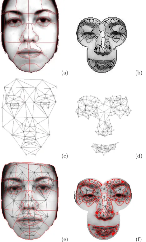
(a) (b)
(c) (d)
(e) (f)
Fig. 5. The model (left) and the image where recognition has to be performed (right). (a), (b): Segmentation superimposed on the image. (c), (d): A subset of the model and the data graphs. We show only edges between adjacent regions to simplify visualization. The real number of edges is much larger since we use complete graphs. (e), (f): A subset of the graphs superimposed on the images.
Figure 5 illustrates this construction. Figures 5(a) and (b) show the model and over-segmented faces, respectively. The corresponding model and image graphs are schematically shown in Figures 5(c) and (d). In order to make visualization easier, only a subset of the edges is shown. Figures 5(e) and (f) show the graphs superimposed on the corresponding images.
We will denote by ND (respectively NM) the set of vertices of GD (respectively
GM), by ED (EM) the set of edges of GD (GM) (in our experiments, the graphs
are complete i.e. ED = ND× ND and EM = NM × NM).
We use crisp attributes in these experiments but fuzzy attributes could also be used as in [24]. Let a be a vertex of GD or GM. The vertex attributes are
defined as the average grey level g(a) of the region represented by a (nor-malized between 0 and 1) and a texture index w(a) computed from wavelet coefficients [11].
Let a and b be two vertices of GD (or of GM). The first edge attribute used is
defined as the vector v(a, b) = pa~pb
2dmax where pa and pb are the centroids of the
regions represented by a and b respectively, and dmax is the largest distance
between any two points of the face region. This attribute is not symmetrical in a and b and therefore edges are directed.
In this section we explore symmetry as a second edge attribute used together with v(a, b), as described below.
5.2 Symmetry attributes
As mentioned in the introduction, when no strict or exact symmetry is verified, then it is meaningful to consider symmetry as a matter of degree, expressed by a symmetry measure. In our case, the regions are crisp sets but, as we have to deal with approximate symmetries, it is still of interest to use a symmetry measure instead of a boolean value. All the results obtained in the previous sections are valid here, considering crisp sets as a particular case of fuzzy sets. Symmetry measures can be used to define a vertex attribute or an edge at-tribute. The first case applies if some objects of the scene are known to be approximately symmetrical. Then it is possible to define a symmetry attribute as the orientation of the symmetry plane of the region and compare these ori-entations in the model and the image to be recognized. Another option for such a scene is to compare the degree of symmetry of regions.
However in the case of facial analysis, the objects taken individually do not have any particular symmetry and therefore we will not use symmetry as a vertex attribute in this paper. On the contrary, some pairs of objects are
approximately symmetrical in the face with respect to the mid-face axis (for example the two eyes, the two eyebrows . . . ). Therefore, it seems natural to consider the degree of symmetry of two regions with respect to the plane (or axis in our case) of symmetry of the face, this leading to an edge attribute. This attribute will constrain a pair of symmetrical regions in the image to be matched with a pair of symmetrical regions in the model. It can be formalized as follows. Let ΠM (respectively ΠD) be the symmetry plane of the model
(respectively of the data). Let a and b be two vertices of the model. Using the symmetry measure σ1, we define the attribute of symmetry of the edge (a, b)
as:
s(a, b) = S1(a, eΠM(b)) (1)
Similarly we define a symmetry attribute for the data as: s(a, b) = S1(a, eΠD(b)). The planes ΠD and ΠM are computed automatically using the
algorithm presented in Section 4. But as the planes are computed on grey-level images, a different symmetry measure is used instead of σA. Let f be a
grey-level image normalized between 0 and 1, eΠ(f ) its reflection with respect
to Π and I = supp(f )∩ supp(eΠ(f )) the intersection of their supports, we
derive the symmetry measure from the L2 distance between images:
σf(Π) = 1−
(P
x∈I(f (x)− eΠ(f )(x))2)1/2
|I|
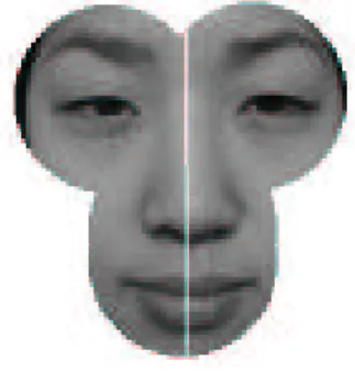
The measure is computed only on the intersection of supports in order not to take into account the background of the image (see for example Figure 6 which shows a face and the detected symmetry axis).
One important property of the symmetry attribute s(a, b) is that it will be zero for most pairs of regions which are not symmetrical, and non-zero only for a small group of approximately symmetrical pairs of regions. This comes from property (P3) presented in Section 2.3. It is illustrated in Figure 7(d). Moreover, regions which are almost symmetrical will lead to a high degree of symmetry. It is illustrated in Figures 7(a) and (b) which show two regions a and b that present a high degree of reflection symmetry. A high degree of symmetry can be identified by the large intersection between a and eΠM(b).
a b (a) b e(b) a (b)
e(b)
a
(c) e(b) a b (d)Fig. 7. (a) Two regions a and b which are approximately symmetrical. (b) s(a, b) is high as a and e(b) (the reflection of b) almost coincide. (c) The second definition (Equation (2)) provides a much higher value than the first one (Equation (1)), because the centroids are very close while the intersection between a and e(b) is reduced. (d) The first definition provides a zero value, while the second definition provides a non zero value.
To evaluate the efficiency of our symmetry attribute, we compared it to an-other attribute computed from the distance between the centroids of the re-gions. Let a and b be two vertices of the model and eΠM(b) be the reflection
of b. Let pa and peΠM(b) be the centroids of the regions represented by a and
eΠM(b) respectively. We define an alternative symmetry attribute of edge (a, b)
as: sd(a, b) = 1− min à 1,d(pa, peΠM(b)) h1+ h2 ! (2) where d(pa, peΠM(b)) denotes the Euclidean distance between the two points and
h1 and h2 are the diameters of a and b, respectively. The symmetry attribute
for the edges of the data graph is defined analogously. The symmetry measure sd(a, b) leads to non-zero values even when the regions a and eΠM(b) do not
in-tersect (see Figure 7(d)). This can be seen as an advantage when one has very small regions. On the other hand, this attribute may indicate high symmetry despite important shape differences between the object and its reflection when the region centroids are very near or coincide (see Figure 7(d)). In Section 5.4, an experimental comparison is presented. The approach presented in [27] also relies on face symmetry axis detection and on a symmetry degree definition. However the following differences can be noted: the symmetry axis computa-tion is done directly using the axes of inertia and the symmetry degree is based
on centroids, like our second attribute but without normalization. Also their approach does not rely on the comparison with a model but on the minimiza-tion of a symmetry-based cost funcminimiza-tion for some particular features. Finally, the method proposed in [27] aims at locating the face and facial features (more specifically, only the centroids of the eyes are found), whereas the application described in the paper allows not only to locate the facial features, but also to segment them (i.e. the image region corresponding to each facial feature).
5.3 Graph matching procedure
Now the next problem to be solved is graph matching. A widely used approach consists in finding an isomorphism between both graphs (or subgraphs). How-ever, the bijective condition is too strong here, and the problem is expressed rather as an inexact graph matching problem [23,6]. Because of the difficulty to segment the image into meaningful entities, no isomorphism can be expected between both graphs. Here, |ND| is generally much larger than |NM|, and we
expect to match several vertices of GD to one vertex of GM, i.e. several image
regions can be assigned to a single model label.
Recognition can then be performed by searching for a homomorphism between GD and GM which satisfies both structural and similarity constraints [25]. A
graph homomorphism is a mapping h : ND → NM such that:
∀(a1
D, a2D)∈ ND2, (a1D, aD2 )∈ ED ⇒ (h(a1D), h(a2D))∈ EM
which imposes a structural constraint on the mapping between edges, and guarantees that each data vertex has exactly one label (i.e. model node). Similarity functions are then used to find the best homomorphism, being thus based on comparison of attributes. A good homomorphism will maximize the similarity between attributes of matched vertices and between attributes of matched edges, or, equivalently, minimize a dissimilarity. The dissimilarity between any two vertices aD ∈ ND and aM ∈ NM is defined here as:
cN(aD, aM) = β|gD(aD)− gM(aM)|+
(1− β)|wD(aD)− wM(aM)|
where gD, wD (gM, wM) are the vertex attributes of graph GD (GM), and β a
parameter for tuning the relative importance of grey level and texture indices. The above dissimilarity measure quantifies the absolute difference between the corresponding image regions w.r.t. the grey values and texture. In our experiments, we set β = 0.6. Parameter values were set experimentally and led to good results for all tested examples. For a different application, these
values might change. It could be interesting, in some future work, to design a learning procedure for all parameters.
The dissimilarity between two edges eD = (a1D, a2D) of ED and eM = (a1M, a2M)
of EM is defined as follows. Firstly, we compute the modulus and angular
differences between v(a1
D, a2D) and v(a1M, a2M) as
φm(eD, eM) = |kv(a1D, a2D)k − kv(a1M, a2M)k|
and
φa(eD, eM) = | cos(θ) − 1|
2 where θ is the angle between v(a1
D, a2D) and v(a1M, a2M)
The dissimilarity measure cE(eD, eM) is defined as:
cE(eD, eM) = γ(δφa(eD, eM)+(1−δ)φm(eD, eM))+(1−γ)|s(a1D, a2D)−s(a1M, a2M)|.
where γ is a weight parameter for tuning the relative importance of the vector attribute and the symmetry attribute (in our experiments, we set γ = 0.6). The above dissimilarity measure quantifies the absolute difference between the corresponding relative position of the respective image regions both w.r.t. the distance between the regions (i.e. length) and orientation (i.e. angle). The factor δ is also a weight parameter, which controls the importance of the modulus and angular differences between the data and the model edges. In our experiments, we have set δ = 0.2 in order to have a good balance between the numerical values of φm and φa.
Based on the vertex and edge dissimilarities, we propose to define a global dissimilarity function as:
f1(h) = α |ND| X aD∈ND cN(aD, h(aD))+ 1− α |ED| X (a1 D,a 2 D)∈ED
cE((a1D, a2D), (h(a1D), h(a2D))), (3)
where α is a weight parameter used for tuning the relative importance of vertex dissimilarity and edge dissimilarity. In our experiments we have set α = 0.4, in order to give more importance to edge information, since it can be expected to be more robust than vertex attributes with respect to the oversegmentation. Several optimization algorithms can be used to compute the minimum of the global dissimilarity function: randomized tree search [7], genetic algo-rithms [19,30] or estimation of distribution algoalgo-rithms (EDAs) [3]. The reader can refer to [6] for a comparison between them. This paper does not focus on the optimization method. Randomized tree search [7] was chosen here to
illustrate our results and should be considered as but one possible example of optimization method, which provides good results.
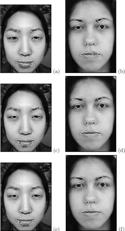
5.4 Results
In order to illustrate the importance of using symmetry to improve the method described in [6], Figure 8 shows the results obtained by the application of the proposed method. Figures 8(a) and (b) show the detection of the eyebrows, eyes, nostrils and mouth as performed by the original method without the symmetry attributes. Some parts have been missed such as the left eye in Figure 8(a) and parts of the mouth in Figure 8(b). The introduction of the symmetry attribute defined by Equation (1) has circumvented these problems, as shown in Figures 8(c) and (d). Finally, the application of the alternative symmetry attribute defined by Equation (2) leads to similar results, which are shown in Figures 8(e) and (f). No significant improvement over the results obtained using Equation (1) can be observed. It is nevertheless worth noting that calculating Equation (1) in practice generally takes much less time since eΠM(b) typically has non-empty intersection with very few regions and the
symmetry should be calculated only for them. On the other hand, the attribute of Equation (2) must be always calculated for all edges in the complete graph. Considering the computational cost, the experimental results, and also the potential problems mentioned in Section 5.2, we suggest to use the attribute of Equation (1).
The computation time is quite reasonable since obtaining the image graph, which includes symmetry axis detection and symmetry measure computation, requires 23 seconds, leading to a total computation time of 7 minutes for the whole graph matching process. Moreover, the intersection computation in the symmetry measure is performed efficiently. For a given object, we can com-pute its intersection with respect to all the other objects using a single min operation on the whole image. As mentioned before, the union computation is only performed for pairs of objects which have a non-zero intersection. This is only a small fraction of all possible pairs. Additionally the computation time could be also reduced using bounding boxes of objects. Finally, the proce-dure is implemented as a mixture of C and matlab routines. In cases where computation time is an important issue, it could be rewritten all in plain C.
6 Conclusion
Since no exact symmetry can usually be expected on real objects, in particular if they are not well defined, we proposed in this paper to study approximate
(a) (b)
(c) (d)
(e) (f)
Fig. 8. Results of recognition (only eyebrows, eyes, nostrils and mouth are shown) on two examples. From top to bottom: without the symmetry attribute ((a) and (b)), with the first definition of the symmetry attribute ((c) and (d)) and with the second definition ((e) and (f)). The symmetry attribute allows to improve the results (mouth, eyebrows). The first definition leads to slightly better results.
symmetries through the definition of symmetry measures. We defined symme-try measures of fuzzy objects based on measures of comparison between the object and its reflection. The choice of an appropriate measure of comparison is based on the required properties for symmetry measures. A comparative study led us to privilege a symmetry measure based on the ratio between a measure of the intersection between the fuzzy set and its reflection and a measure of their union.
Another contribution of this paper consists of an algorithm to compute the best symmetry plane of a 3D fuzzy object. Thanks to a reasonable initialization based on the inertia axes, it iteratively converges towards the global optimum. These two aspects of our work have been applied on a facial feature recognition problem. The face symmetry axis has been found using the proposed optimiza-tion method. The recognioptimiza-tion problem is expressed as an inexact graph match-ing where one graph represents a face model and the second graph represents the image where recognition has to be performed. Vertices represent image re-gions and edges represent spatial relations between these rere-gions. Symmetry measures are used as edge attributes, and contribute to improve recognition results by favoring associations of symmetrical regions in the model with sym-metrical regions in the image.
Multiple perspectives of this work can be foreseen. First, we expect that a similar approach could be used for other recognition problems, such as brain structures. Another possible use of the symmetry axis or plane could be to guide a registration procedure to get an initial match between the model and the image. The proposed symmetry measure has also been used by Letournel et al. [16] to define a feature for the evaluation of segmentations in aerial imaging. Finally, another interest of this work is to derive spatial relationships referring to symmetry. This can be particularly useful for applications where directional relations like “on the left” are not absolute but relative to a symmetry plane of some object [8].
Appendix
We give here the main lines of the proofs of the properties of the measures used in Section 3. Proofs for S1 S1(A, B) = P x∈Ω>(µA(x), µB(x)) P x∈Ω⊥(µA(x), µB(x))
Proposition 1 Property (P2) holds if and only if > = min and ⊥ = max. Proof One has>(µA(x), µB(x))≤ ⊥(µA(x), µB(x)) for all x∈ Ω. Therefore,
S1(A, B) = 1 ⇐⇒ >(µA(x), µB(x)) =⊥(µA(x), µB(x)) for every x∈ Ω.
Since for every x∈ Ω:
>(µA(x), µB(x))≤ min(µA(x), µB(x)) ≤ max(µA(x), µB(x))≤ ⊥(µA(x), µB(x)),
one has:
S1(A, B) = 1 ⇐⇒ A = B and > = min and ⊥ = max .
2 Proposition 2 Property (P3) is fulfilled for t-norms “minimum” and “prod-uct” but is not for “drastic” and “Lukasiewicz” ones [9].
Proof
S1(A, B) = 0 ⇐⇒ >(µA(x), µB(x)) = 0 for all x∈ Ω.
For “minimum” and “product” t-norms, one has
min(µA(x), µB(x)) = 0 ⇐⇒ µA(x) = 0 or µB(x) = 0,
µA(x)µB(x) = 0 ⇐⇒ µA(x) = 0 or µB(x) = 0
and therefore (P3) holds. For “drastic” and “Lukasiewicz” t-norms, one can have µA(x)6= 0 and µB(x)6= 0 but >(µA(x), µB(x)) = 0 (for example,
µA(x) = µB(x) = 0.5). Therefore (P3) does not hold. 2
Proposition 3 Properties (P4) and (P5) are fulfilled.
Proof The proof is given here for the translation only, since for the rotation it is similar. S1(A + v, B + v) = P x∈Ω>(µA+v(x), µB+v(x)) P x∈Ω⊥(µA+v(x), µB+v(x))
By definition one has µA+v = µA(x− v). Therefore
S1(A + v, B + v) = P
x∈Ω>(µA(x− v), µB(x− v)) P
x∈Ω⊥(µA(x− v), µB(x− v))
Substituting x− v with x one gets S1(A + v, B + v) = S1(A, B) The proofs
Proofs for S2 S2(A, B) = 1 |Ω|× X x∈Ω >(µA(x), µB(x)) ⊥(µA(x), µB(x))
Proposition 4 S2 satisfies (P2) if and only if > = min and ⊥ = max but
does not satisfy (P3).
Proof The proof for (P2) is the same as for S1.
(P3): Let us consider two fuzzy sets A and B with disjoint supports such that supp(A) ∪ supp(B) 6= Ω. Then there exists x in Ω such that µA(x) = µB(x) = 0 and therefore S2(A, B)6= 0. 2
Proofs for S4
S4(A, B) = max
x∈Ω >(µA(x), µB(x)).
Proposition 5 S4 does not satisfy (P2).
Proof If A is a normalized fuzzy set, one has S(A, A) = 1. However, the converse implication is false. If there exists an element x such that µA(x) =
µB(x) = 1 then S4(A, B) = 1, even if A6= B. 2
Proofs of Section 3.2
For all these measures, it is easy to check that properties (P1), (P2), (P4) and (P5) hold.
Proofs for S5
S5(A, B) = 1− kA − Bk1
|Ω| .
Proposition 6 This measure does not satisfy property (P3). Proof Suppose that sets A and B have disjoints supports. Then:
kA − Bkp = Ã X x∈Ω µA(x)p+ µB(x)p !1p
X x∈Ω µA(x)p+ µB(x)p ≤ |Ω| Thus, if P x∈ΩµA(x)p+ µB(x)p > 1, kA − Bkp <|Ω| 2 Proofs for S6 S6(A, B) = 1− kA − Bkp (P x∈ΩµA(x)p+ µB(x)p) 1 p
Proposition 7 Measure S6 satisfies property (P3).
Proof Suppose that sets A and B have disjoint supports. Then S6(A, B) = 0,
since kA − Bkp = Ã X x∈Ω µA(x)p+ µB(x)p !1p .
The converse is also true since S6(A, B) = 0 =⇒ ∀x ∈ Ω, |µA(x) −
µB(x)|p = µA(x)p+ µB(x)p =⇒ ∀x ∈ Ω, µA(x) = 0 or µB(x) = 0. 2
References
[1] B.A. Ardekani, J. Kershaw, M. Braun, and I. Kanno. Automatic detection of the mid-sagittal plane in 3D brain images. IEEE Transactions on Medical Imaging, 16(6):947–952, 1997.
[2] O. Ayinde and Y.-H. Yang. Region-based face detection. Pattern Recognition, 35(10):2095–2107, October 2002.
[3] E. Bengoetxea, P. Larranaga, I. Bloch, and A. Perchant. Solving graph matching with EDAs using a permutation-based representation. In P. Larranaga and J. A. Lozano, editors, Estimation of Distribution Algorithms: A New Tool for Evolutionary Computation, chapter 12, pages 239–261. Kluwer Academic Publisher, Boston, Dordrecht, London, 2001.
[4] I. Bloch. On fuzzy distances and their use in image processing under imprecision. Pattern Recognition, 32(11):1873–1895, 1999.
[5] B. Bouchon-Meunier, M. Rifqi, and S. Bothorel. Towards general measures of comparison of objects. Fuzzy Sets and Systems, 84(2):143–153, 1996.
[6] R.M. Cesar, E. Bengoetxea, and I. Bloch. Inexact graph matching using stochastic optimization techniques for facial feature recognition. In International Conference on Pattern Recognition, Qu´ebec, Canada, 2002. [7] R.M. Cesar and I. Bloch. First results on facial feature segmentation and
recognition using graph homomorphisms. In SIARP 2001, pages 95–99, Florianapolis, Brazil, October 2001.
[8] O. Colliot, I. Bloch, and A.V. Tuzikov. Characterization of approximate plane symmetries for 3D fuzzy objects. In Information Processing and Management of Uncertainty IPMU, volume 3, pages 1749–1756, Annecy, France, July 2002. [9] D. Dubois and H. Prade. Fuzzy Sets and Systems, Theory and Applications.
Academic Press, New-York, 1980.
[10] B. Fasel and J. Luettin. Automatic facial expression analysis: a survey. Pattern Recognition, 36(1):259–275, January 2003.
[11] R.S. Feris, V. Kr¨uger, and R.M. Cesar. Efficient real-time face tracking in wavelet subspace. In Proc. Second International Workshop on Recognition, Analysis and Tracking of Faces and Gestures in Real-time Systems, 8th IEEE International Conference on Computer Vision (RATFGRTS ICCV 2001 -Vancouver, Canada), pages 113–118, 2001.
[12] T. Gerstenkorn and J. Man’ko. Correlation of intuitionistic fuzzy sets. Fuzzy Sets and Systems, 44:39–43, 1991.
[13] H. J. A. M. Heijmans and A. Tuzikov. Similarity and symmetry measures for convex shapes using Minkowski addition. IEEE Transactions on Pattern Analysis and Machine Intelligence, 20(9):980–993, 1998.
[14] L.K. Hyung, Y.S. Song, and K.M. Lee. Similarity measure between fuzzy sets and between elements. Fuzzy Sets and Systems, 62:291–293, 1994.
[15] T. Kondo and H. Yan. Automatic human face detection and recognition under non-uniform illumination. Pattern Recognition, 32:1707–1718, 1999.
[16] V. Letournel, B. Sankur, F. Pradeilles, and H. Maˆıtre. Feature extraction for quality assessment of aerial image segmentation. In ISPRS, Commission III, PCV, volume XXXIV, pages 199–204, Graz (Austria), sep 2002.
[17] X. Liu. Entropy, distance measure and similarity measure of fuzzy sets and their relations. Fuzzy Sets and Systems, 52:305–318, 1992.
[18] G. Marola. On the detection of the axes of symmetry of symmetric and almost symmetric planar images. IEEE Transactions on Pattern Analysis and Machine Intelligence, 11:104–108, 1989.
[19] Z. Michalewicz. Genetic Algorithms + Data Structures = Evolution Programs. Springer Verlag, Berlin Heidelberg, 1992.
[20] P. Minovic, S. Ishikawa, and K. Kato. Symmetry identification of a 3D object represented by octree. IEEE Transactions on Pattern Analysis and Machine Intelligence, 15(5):507–514, 1993.
[21] D. O’Mara and R. Owens. Measuring bilateral symmetry in digital images. In Proceedings of TENCON’96 IEEE Conference: Digital Signal Processing Applications, volume 1, pages 151–156, 1996.
[22] C.P. Pappis and N.I. Karacapilidis. A comparative assessment of measures of similarity of fuzzy values. Fuzzy Sets and Systems, 56:171–174, 1993.
[23] A. Perchant and I. Bloch. A new definition for fuzzy attributed graph homomorphism with application to structural shape recognition in brain imaging. In 16th IEEE Intrumentation and Measurement Technology Conference, volume 3, pages 1801–1806, 1999.
[24] A. Perchant and I. Bloch. Semantic spatial fuzzy attribute design for graph modeling. In IPMU 2000, volume III, pages 1397–1404, Madrid, Spain, 2000. [25] A. Perchant and I. Bloch. Fuzzy morphisms between graphs. Fuzzy Sets and
Systems, 128(2):149–168, 2002.
[26] W.H. Press, S.A. Teukolsky, W.T. Vetterling, and B.P. Flannery. Numerical Recipes in C. 2nd Edition. Cambridge University Press, Cambridge, 1992. [27] E. Saber and A. M. Tekalp. Face detection and facial feature extraction using
color, shape and symmetry-based cost functions. In Proceedings of the 13th International Conference on Pattern Recognition, 1996,, volume 3, pages 654– 658, 1996.
[28] A. Tversky. Features of similarity. Psychological Review, 84:327–352, 1977. [29] W.-J. Wang. New similarity measures on fuzzy sets and on elements. Fuzzy
Sets and Systems, 85:305–309, 1997.
[30] D. Whitley and J. Kauth. GENITOR: A different genetic algorithm. In Proceedings of the Rocky Mountain Conference on Artificial Intelligence, volume 2, pages 118–130, 1988.
[31] K.-W. Wong, K.-M. Lam, and W.-C. Siu. An efficient algorithm for human face detection and facial feature extraction under different conditions. Pattern Recognition, 34(10):1993–2004, October 2001.
[32] H. Zabrodsky, S. Peleg, and D. Avnir. Symmetry as a continuous feature. IEEE Transactions on Pattern Analysis and Machine Intelligence, 17:1154– 1166, 1995.
[33] W. Zhao, R. Chellappa, A. Rosenfeld, and P.J. Phillips. Face recognition: A literature survey. Technical report, UMD CfAR, 2000. URL: citeseer.nj.nec.com/374297.html.
[34] R. Zwick, E. Carlstein, and D.V. Budescu. Measures of similarity among fuzzy concepts : A comparative analysis. International Journal of Approximate Reasoning, 1:221–242, 1987.