HAL Id: hal-03197762
https://hal.archives-ouvertes.fr/hal-03197762
Submitted on 14 Apr 2021HAL is a multi-disciplinary open access archive for the deposit and dissemination of sci-entific research documents, whether they are pub-lished or not. The documents may come from teaching and research institutions in France or abroad, or from public or private research centers.
L’archive ouverte pluridisciplinaire HAL, est destinée au dépôt et à la diffusion de documents scientifiques de niveau recherche, publiés ou non, émanant des établissements d’enseignement et de recherche français ou étrangers, des laboratoires publics ou privés.
Financing the newsvendor with preferential credit: bank
vs. manufacturer
Yuxiang Cheng, Desheng Dash Wu, David Olson, Alexandre Dolgui
To cite this version:
Yuxiang Cheng, Desheng Dash Wu, David Olson, Alexandre Dolgui. Financing the newsvendor with preferential credit: bank vs. manufacturer. International Journal of Production Research, Taylor & Francis, 2020, pp.1 - 20. �10.1080/00207543.2020.1759839�. �hal-03197762�
https://doi.org/10.1080/00207543.2020.1759839
International Journal of Production Research, Published online: 02 Jul 2020
Financing the newsvendor with preferential credit:
Bank vs. Manufacturer
Yuxiang Cheng
Desheng Wu
David L. Olson
Alexandre Dolgui
This version: 5 June, 2020
Yuxiang Cheng is from Economics and Management School at University of Chinese Academy of Sciences, email: chengyuxiang18@mails.ucas.ac.cn. Desheng Wu is from Economics and Management School at University of Chinese Academy of Sciences and Stockholm Business School at Stockholm University, email: dash.wu@gmail.com. David L. Olson is from College of Business Administration at University of Nebraska-Lincoln, email: dolson3@unl.edu. Alexandre Dolgui is from Department of
Automation, Production and Computer Sciences at IMT Atlantique, email: alexandre.dolgui@imt-atlantique.fr.
Financing the newsvendor with preferential credit:
Bank vs. Manufacturer
Abstract
This paper examines how preferential credit based on retailers’ credit line impacts on capital-constraint retailer’s operational decisions. We consider a condition of loan competition when banks and manufacturers offer preferential credit to capital-constraint retailers in the newsvendor model. Different credit lines and discounted rates of preferential credit mainly involve in retailers' exogenous collateral and risk preference of banks and manufacturers in our model. We investigate impacts of bank financing, trade credit, and portfolio credit (financing from both bank credit and trade credit with different ratios) on retailer's inventory decision with different cases that the retailer's financing amounts exceed credit line or not. We derive the equilibrium wholesale price, expected sale price, and order quantity when retailers face with different conditions of collaterals and institutes' risk preferences facing with market risk. A debt-financed retailer favours items with trade credit compared to bank financing, especially in conditions when its sourcing demand is great and when it finances from high-risk preference institutes. Retailer prefers to using the loan with high trade credit ratio when he opts portfolio credit conditions.
Keywords: supply chain financing; default risk; preferential credit; trade credit; bank finance.
1. Introduction
Trade credit, offered by suppliers to retailers to meet their purchasing demand, is a common component of supply chain contracts. According to the Financial Times, 90% of international merchandise trade in America was financed by trade credit, amounting to $25 trillion1. Boeing Company allows financing to hundreds of capital-constrained enterprises through trade credit2. Over the period, 2003-2012 nearly 202,696 small- and medium-sized enterprises (SMEs) across 13 European countries used trade credit for sourcing (McGuinness et al., 2018). Trade credit also plays a vital role in alleviating pressures from financial shortage to SMEs, especially in developing countries (Fisman and Love, 2003; Jacobson and Schedvin, 2015; Wu et al., 2019). Feess and Thuyn (2014) used a game-theoretic model to analyze surplus division in supply chains. Van dere Vliet et al. (2015) provided a periodic review inventory model with reverse factoring. In China, trade credit might be the only method for capital constraint enterprises to satisfy their financing demands. These SMEs' trade credit comes primarily from big Internet companies such as Baidu, Alibaba, and Tencent.
Trade credit has some advantages compared to traditional bank financing for enterprises. It could increase order quantities for capital-constrained retailers (Wu et al., 2019); benefits firms facing with uncertainty (Yin et al., 2015; Wu et al., 2018); reduce financing cost (Melnyk et al., 2014); improve buyer’s bargaining power (Klapper et al., 2011); define default risk quicker (Smith, 1987), and lower transaction costs (Emery, 1984; Gao et al., 2018) identified optimal Stackelberg strategies for peer-to-peer lending in supply chains. Most works (Kouvelis and Zhao, 2011; Chod, 2016; Huang et al., 2019) consider original trade credit in supply chains to finance inventory.
In 2019 DSI annual conference, supply chain financing (SCF) attracts wide attention. Shrivastava and Rogers offered the keynote named “Technology Powering the Evolution of Supply Chain Financing” to highlight the importance of SCF to firms’ development.3 The firms operate is not isolation. They are always embedded in
powerful network with other firms. Also, in this annual conference, Wetzel and Hofmann (2019) analyzed the efficiency and effectiveness of the financial supply chain
1 See: https://www.ft.com/content/9ebcdfaa-b012-11dd-a795-0000779fd18c
2 See: http://boeing.mediaroom.com/2012-02-17-Boeing-Citi-Start-Export-Import-Bank-Supplier-Financing-Program 3 See: https://decisionsciences.org/two-keynotes-to-highlight-2019-conference/
network. Carnovale et al. (2019) examined the effect that network power and cohesion have on a firm’s financial performance in dynamic supply chain network structure. Accordingly, different trade credit policies which can improve financing efficiency and facilitate competition, would be generated in the network of firms and banks.
Nowadays, one type of trade credit named preferential trade credit is often given to firms for series reasons, such as attracting purchase, supporting industry development, and building a long-term cooperative relationship. It develops remarkably in recent years. In Azerbaijan, a local furniture company named Saloglu obtained a preferential credit worth of 5.9 million dollars on February 2, 20194. Firms with high-quality operational conditions, or supported by the government have access to financing inventory from banks with preferential credit, which has low loan interests. According to the report of the People's Bank of China (PBC) in 2018, that banks provided long-term preferential funds with discounted interest rates to financial institutions through targeted RRR cuts, targeted medium-term loan facilities, and refinancing, leading to an increase in preferential loans for SMEs. At the end of 2018, the balance of SMEs preferential loans was 8 trillion yuan, increasing 18%, with a growth rate of 8.2%5. Additionally, the China Development Bank (CDB) will provide a preferential loan of no less than 200 billion yuan to provide sufficient protection for the integration of transportation and tourism companies during the "Thirteenth Five-Year Plan" period6.
Apart from China, The National Development Bank PLC (NDB Bank) in Sri Lanka offered preferential loans, sometimes with free collateral, to SMEs in industries such as agriculture, fisheries, textile, handicrafts, floriculture, construction, retail, etc7. Due to the development of preferential credit, this is important to investigate its influences on retailers' inventory decisions. Little literature considers the impacts of preferential credit on supply chain management when retailers are capita-constraint. We consider the following questions when retailers source in preferential credit.
Based on the development of preferential credit, which sourcing for SMEs will help them to increase more benefits? Is the manufacturer's preferential trade credit more beneficial to retailers compared to the bank's preferential loan? When manufacturers consider to compete with banks to gain lending for retailers, they may offer discount
4 See: https://caspiannews.com/news-detail/made-in-azerbaijan-expected-to-diversify-economy-2019-2-1-28/ 5 See: http://finance.sina.com.cn/roll/2019-01-16/doc-ihqfskcn7466096.shtml
6 See: http://www.cb.com.cn/index/show/jj/cv/cv1152735797
trade credit based on the retailer’s operating conditions. Banks would like to lend to retailers that owe high-quality assets. In this way, it could bring more revenue to themselves. Thus, banks will also offer discount bank interest rates to attract retailers to source. Questions attract us, including what would happen if retailers sourced in these competing circumstances, and how does preferential credit by manufacturers and banks to retailers affect the supply chain?
Motivated by these questions, this paper aims to examine the impacts of preferential credit given by banks and manufacturers. Capital-constraint retailers with high-quality assets or belong to state-supported industries could choose bank credit or manufacturer credit facing with different discount interest rates. At the end of the transaction, retailers pay back loans and interest. However, the default will happen if retailers’ revenue could not amount to its payment due to market risk, which means the condition that retailers may not sell its inventories extremely. When we consider default risk, banks would evaluate retailer’s quality and design contracts, including preferential credit lines for the convenience of the retailer, according to bank risk preference to retailers’ default and retailers’ collateral assets, which are hard to achieve liquidity in the model. Besides, the credit line evaluated by banks can be observed by the manufacturer (we consider this a non-information asymmetry market). The manufacturer would offer a discount trade credit based on its risk preference to default risk. This paper tries to answer the questions: (1) will the bank and manufacturer risk preference affect a retailer’s sourcing decision based on preferential credit? (2) how does the retailer’s asset quality (collateral) impact on sourcing strategy? (3) could the preferential credit benefit the retailer when the retailer finance from bank credit or trade credit?
To answer the first question, we analyze a Stackelberg game that involves three parties: a manufacturer, a capital-constrained retailer, and a bank. We consider different risk preferences for banks and manufacturers offering credit to the retailer. Due to credit line differences, we identify two cases in bank credit. Case 1 is the situation where the bank loan exceeds the credit line. Case 2 is the situation where the bank loan is lower than the credit line. We conclude that with an increase in bank risk preference, retailer order quantity increases under Case 1. However, optimal order quantity may not change with bank risk preference in Case 2. Besides, the manufacturer’s risk preference may have no effect on order quantity under trade credit. The discount interest rate leads to a higher wholesale price, which transfers the retailer's profits to the manufacturer. When we focus on portfolio credit (finance both from bank and manufacture), there are two
scenarios for the retailer to source. Scenario I: bank loan is higher than the credit line under portfolio credit. Scenario II: bank loan is lower than the credit line under portfolio credit. A high manufacturer's risk preference hurts the retailer in scenario I. There is no difference for the retailer's ordering decision in scenario II. The optimal quantity for the retailer to order is between bank credit and trade credit levels.
To answer the second question, we explore the influences of the retailer's collateral based on a decentralized supply chain. In a decentralized supply chain, the retailer's profit will decrease, especially on the condition of opting trade credit. The benefit of preferential credit primarily transfers to the manufacturer, leading to the improvement of the manufacturer's profit. However, with an increase in collateral, the effect on total supply chain profit is positive.
To answer the third question, we compare the impacts of preferential credit in bank credit and trade credit. We find that benefit transferring would be extended with trade credit. The benefit from discounting interest rates completely transfers to the manufacturer under trade credit, which is also similar to bank credit in some certain. However, the retailer could be motivated to order more quantity in trade credit. Namely, preferential credit has a positive effect on retailers.
Our paper reveals two critical managerial implications. Firstly, preferential credit cannot motivate retailers to order more under trade credit because the benefits will transfer to the manufacturer through a higher wholesale price. Secondly, the retailer's collateral cannot lead to more profit to the retailer, but it can improve total supply chain efficiency. If retailers with high-quality assets finance through banks, a higher risk preference bank would be better.
The rest of this paper is structured as follows. Relevant published literature is reviewed in Section 2. Section 3 proposes the basic model and assumptions. Stackelberg equilibrium with bank credit, trade credit, and portfolio credit are derived respectively in Section 4, Section 5, and Section 6. Besides, section 7 demonstrates managerial insights through computational study. We summarize the article in Section 8. Proofs are collected in the Appendix.
2. Literature review
When considering the impact of different supply chain financing schemes on asymmetric markets, our paper is related to the following research streams: models with
decisions under capital constraint, comparative models of bank financing under stochastic demand, and price-setting newsvendor problem.
The first stream considers supply chain decisions under capital constraint and trade credit. Xu and Birge (2004) gave a newsvendor framework related to a capital-constrained retailer and analyzed how capital constraint and capital structure could impact management decisions. The theory of trade credit in capital constraint was considered by Burkart and Ellingsen, 2004; Gupta and Dutta, 2011; Breza and Liberman, 2013; Zhan et al., 2019. Dada and Hu (2008) considered a capital constraint newsvendor model where the retailer borrows funds at a low-interest rate, leading to drop in retailer equity. Kouvels and Zhao (2011) explored retailer bankruptcy risk when the retailer was financially constrained and failed to repay the loan. With bankruptcy risk, the wholesale price would be raised. When bankruptcy risk is not present, the manufacturer may keep the wholesale price stable. Trade credit in competitive markets has been found to bring extra benefits to supply chains (Rice and Strahan, 2010; Peura et al., 2017; Chod et al., 2019). Chod (2016) proposed a model to study how debt financing distorted a retailer's inventory decision and developed a first-best inventory decision. All these papers consider capital constraints in the supply chain no matter whether the constraint is on the retailer or the manufacturer. However, multiple source finance by a retailer is neglected, and preferential credit from heterogeneous manufacturers or lenders has not been considered in various of literature.
The second stream involves models comparing bank finance alternatives under stochastic demand in supply chains. Trade credit is compared to bank credit in recent papers such as Gupta (2008) and Zhou and Groenevelt (2007). Kouvelis and Zhao (2012) considered a risk-neutral supplier financing a retailer within bankruptcy risks. A supplier with an early payment discount scheme was proposed as a decision framework to analyze decisions. Their work concluded that under optimal trade credit contracts, both the supplier's profit and supply chain's efficiency gained improvements. Deng et al. (2018) established a model involving financing multiple heterogeneous suppliers and demonstrated that buyer finance is better even if its own unit capital opportunity cost is higher than the bank risk-free interest rate. Doumpos and Zopounidis (2011) proposed an evolutionary algorithm to assess the risk of credit portfolios in firms, which examines default risk in the supply chain. Yang and Birge (2018) demonstrated a portfolio credit impact related to bankruptcy when the retailer's cash level was low. The result demonstrated that trade credit allows the supplier to take advantage of the retailer's
financial weakness, yet it may also benefit both parties (retailer and supplier). These sources investigate the bank loan effect in the supply chain but do not consider the loan competition between banks and manufacturers.
The last stream of this paper is on the price-setting newsvendor problem. Related literature to consider price factor into newsvendor problems are commonly involved in two different demand models, such as additive and multiplicative forms (Petruzzi and Dada 1999; Granot and Yin, 2005; Jammernegg and Kischka, 2013; Hu and Su, 2018). The additive demand model represents that the variance of demand is independent of price (Gallego and van Ryzin, 1994; Kyparisis and Koulamas, 2018). However, demand in multiplicative forms is a descend function with price (Lau et al., 2008). The existing papers usually consider that the price is exogenous. However, distinctive from such papers, we endogenous the price in newsvendor problem based on a linear demand model, which means that the price could be decided based on stochastic demand and retailers’ inventory policy.
In our work, we also study heterogeneous bank’s and manufacturer's risk preferences to the retailer's default. The bank and manufacturer offer preferential credit to attract retailer’s financing. Due to the constraint of working capital, the retailer who face with stochastic market demand could not pay back the loan and interest when risk event happens. In this case, it will cause default on their payments. The mostly related article compared to our paper is Kouvelis and Zhao (2017). However, Kouvelis and Zhao (2017) consider the credit rating to yield different discount interest rate financing. They ignore the risk preference’s effect and the different risk preferences impacts between the bank and the manufacturer, which is significantly essential to inventory decisions. The risk-averse may impact the operational condition of retailers as many works proposed (Gan et al., 2005; Choi et al., 2008 and Yang et al., 2018). We consider this perspective to examine the effect of the supply chain when the default event happens. We find that preferential credit may not particularly benefit the retailer under trade credit. With portfolio credit, the retailer's situation would be worse compared to trade credit when he faces higher manufacturers' risk preference level.
3. Model and notation
We now consider a supply chain system consisting of three parties: a capital constraint (hereafter referred to as “he” in the following), a manufacturer (she) which owes sufficient capital, and a competitive commercial bank (it). In our model, the retailer
decides the optimal order quantity to maximize his profit. The manufacturer decides the wholesale price in the supply chain. In the product market, the retailer faces stochastic demand denoted by D with a distribution function F(D), which is continuously differentiable. The general failure rate is defined as 𝐻(𝐷) = 𝐷𝑓(𝐷)
𝐹(𝐷)
̅̅̅̅̅̅̅, with a hazard rate
ℎ(𝐷) =𝑓(𝐷)
𝐹(𝐷)
̅̅̅̅̅̅̅. Assume 𝐻(𝐷) and ℎ(𝐷) are increasing in D (Kouvelis and Zhao, 2012).
Capital-constraint retailers has not enough initial capital to pay order quantity immediately. Bank credit offered by bank and trade credit offered by manufacturer are useful for capital-constraint retailer to source. Under the competitive credit market, the bank would provide preferential credit to high-quality enterprises according to their collateral in order to attract prime loans and earn profit. In other words, the bank would give loans with discount interest rates and evaluate preferential credit lines based on the retailer's mortgage asset. This mortgage asset is hard to realize liquidity to pay financing costs in our assumption. The preferential credit line (𝐿𝐶) is determined by the banks,
depending on collateral (TC) and mortgage rate (g). Besides, collateral is exogenous due to it is hard to realize liquidity in our assumption, which means it will not be as payment to debt. Namely, default risk exists, but there is no bankruptcy to the retailer. Furthermore, this part of the loan is convenient and easy for the retailer to lend, meaning that it has high fluidity. We assume that retailers can borrow this part of preferential credit balance to pay trade credit. Thus, when the manufacturer observes the credit balance that the retailer has, she would give a discounted trade credit to the retailer. Also, the discount rate depends on the risk preference level of bank and manufacturer to retailer’s default, considered as h and e. We have the bank interest rate as follows when bank loan 𝐿𝐵 is
lower than 𝐿𝐶.
𝑟𝐶,𝐵 = 𝑟𝐵− 𝑢 × ℎ × 𝐿𝐶. (1)
𝐿𝐶 = 𝑔 × 𝑇𝐶. (2)
𝑟𝐶,𝐵 is the discount interest rate of banks in the credit line. 𝑟𝐵 means the bank interest rate apart from the credit line. 𝑢 is a the parameter of the discount rate, which represents the discount degree after bank’s consideration for risk evaluation and preferential credit line. In our model, we use multiplication rule to reflect the discount value, which is common in supply chain finance fields (Kouvelis and Zhao, 2012).
Similarly, the manufacturer decides the discount interest rate based on normal interest rate 𝑟𝑀 after she considering the loan amount and risk preference. Thus, we obtain the
𝑟𝐶,𝑀 = 𝑟𝑀− 𝑒 × 𝑢(𝑔𝑇𝐶 − 𝐿𝐵). (3) Focused on this equation, 𝑟𝐶,𝑀 is the discount interest rate of trade credit. 𝐿𝐵 is the bank loan, and 𝑟𝑀 means the normal trade credit interest rate. We assume that 𝑟𝑀 ≥ 𝑟𝐵 if the retailer does not use a bank loan. The 𝐿𝐵= 0, we have
𝑟𝐶,𝑀 = 𝑟𝑀− 𝑔 × 𝑒 × 𝑢 × 𝑇𝐶. (4)
Then, we know that the discount interest rate of trade credit only depends on the the normal trade credit interest rate (𝑟𝑀), mortgage rate (g), the parameter of the discount rate (u), and collateral (TC) when the retailer only finances inventory from trade credit.
In the market, companies could decide the product's price to attract consumers, which match the demand with retailers' inventory. Thus, in our model, we relax the assumption of unchanged price and assume that the retailer could decide the price according to the relationship between expected stochastic demand (D) and order quantity (q). We consider in linear demand model, which could be written as follows.
𝑝 = 𝑎 − 𝑏 × min(𝐷, 𝑞). (5)
The expected sales price E(p) is 𝑎 − 𝑏 ∫ 𝐹̅(𝐷)𝑑𝐷0𝑞 , which is easy to prove. The retailer considers the expected sales price to maximize profit in our model. The retailer orders q units of the product at wholesale price w. With stochastic demand, when q is over-ordered and exceeds the market’s demand, the overage would be sold by a buyback price s. The manufacturer has a cost of k to produce products, with E(p)> w>k>s. For the capital-constrained retailer, the working capital is B and 𝑤𝑞 ≥ B, the retailer needs to finance from the bank or the manufacturer and repays (𝑤𝑞 − 𝐵)(1 + 𝑟) in the end. We assume the retailer’s quality is adequate, and collateral TC is high, and there is no retailer bankruptcy. However, default will happen when retailers could not return loans and their interest.
In this study, we derive in the Stackelberg equilibrium to examine the effect of different risk preferences and collateral levels. Key notations are collected in Table 1.
[Please insert Table 1 about here]
4. Bank financing
In this section, we analyze the operational supply chain decision under bank loan in two different cases. In case 1, the amount of the retailer's bank loan is in a low level and does not exceed the credit line. We define it as 𝐿𝐵 ≤ 𝑔𝑇𝐶. For case 2, the retailer orders lots of quantity. The amount of loan is more than the credit line, which is 𝐿𝐵 ≥ 𝑔𝑇𝐶.
According to these two different cases, the retailer decides the optimal order quantity based on different profit functions.
4.1 The retailer’s problem
Before the marketing period, the capital-constrained retailer needs to pay wq to the manufacturer. However, the retailer only has initial capital T available. He lends 𝐿𝐵 from
the bank. At the end of this period, he needs to pay 𝐿𝐵(1+r) to the bank, and r is determined given the different cases. In the stochastic demand market, the minimum product demand is D and the maximum demand is retailers’ order quantity q. When retailers can not sale the product totally, the surplus product would be recycled. The buyback price is s. Namely, the retailer’s revenue depends on two aspects, the sale revenue and the buyback revenue of surplus products. It can be written as follows:
𝐸(𝑝) × 𝑚𝑖𝑛[𝑞, 𝐷] + 𝑠 × max[𝑞 − 𝐷, 0]. (6)
Where 𝐸(𝑝) = 𝑎 − 𝑏 ∫ 𝐹̅(𝐷)𝑑𝐷0𝑞 .
Due to the different amounts of bank credit, we would need to consider two cases to discuss the retailer’s problem.
Case 1. Bank loan does not exceed the credit line, 𝐿𝐵 ≤ 𝐿𝐶.
In this condition, the bank offers the retailer with a preferential credit based on the retailer's collateral and mortgage rate. Thus, the retailer's payment to the bank at the end of the period is (𝑤𝑞 − 𝑇)(1 + 𝑟𝐶,𝐵). Combined with Equation (6), the retailer’s profit is as follows:
𝐸(𝑝) × 𝑚𝑖𝑛[𝑞, 𝐷] + 𝑠 × max[𝑞 − 𝐷, 0] − (𝑤𝑞 − 𝑇)(1 + 𝑟𝐶,𝐵) − 𝑇. (7) It is easy to verify that the expected sales price E(p) is 𝑎 − 𝑏 ∫ 𝐹̅(𝐷)𝑑𝐷0𝑞 when we
consider the expected value for Equation (5). Then, we take the expected value for Equation (7). The expected profit of the retailer can be simplified as follows:
𝜋𝑟,𝐵,1 = 𝐸(𝑝)𝑞 − (𝐸(𝑝) − 𝑠) ∫ 𝐹(𝑥)𝑑𝑥 𝑞
0 − (𝑤𝑞 − 𝑇)(1 + 𝑟𝐶,𝐵) − 𝑇. (8)
Where 𝐸(𝑝) = 𝑎 − 𝑏 ∫ 𝐹̅(𝐷)𝑑𝐷0𝑞 , 𝑟𝐶,𝐵 = 𝑟𝐵− 𝑢 × ℎ × 𝐿𝐶, and 𝐿𝐶 = 𝑔 × 𝑇𝐶.
From Equation (8), we capture the expected the profit of retailers depending on retailers’ order quantity, his initial capital, buyback price, the expected sale price, the wholesale price, and the discount interest rate of banks. In order to find the optimal order quantity by maximizing the retailer’s profit, we obtain the Proposition 1.
Proposition 1. In a decentralized supply chain, when the retailer is given preferential
credit from a bank (with a given wholesale price), the optimal order quantity 𝑞𝐵,1∗ satisfies the first-order optimality condition of its expected profit function, which is given as follows:
𝑎 − 2𝑏 ∫𝑞𝐵,1∗ 𝐹̅(𝐷)𝑑𝐷
0 − 𝑠 =
𝑤(1+𝑟𝐵−𝑔𝑢ℎ𝑇𝐶)−s
𝐹̅(𝑞𝐵,1∗ ) . (9)
When the bank loan is lower than the credit line, the optimal order quantity based on a given wholesale price can be affected by wholesale price (w), bank interest rate (𝑟𝐵), risk preference level of bank (ℎ), and retailer's collateral (TC).
Corollary 1. (Effect of bank decision) In case 1: (i) 𝑞𝐵,1∗ is increasing in bank risk preference, 𝜕𝑞𝐵,1 ∗ 𝜕ℎ > 0;(ii) 𝑞𝐵,1 ∗ is decreasing in 𝑟 𝐵, 𝜕𝑞𝐵,1∗ 𝜕𝑟𝐵 < 0.
The intuition behind Lemma 2 is as follows: When the bank improves the interest rate, the loan cost for the retailer is raising. Retailer orders lower order quantity; However, when retailer finances from a higher risk preference bank, which would give a higher discount, due to the cost of finance is reduced, the retailer would want to order more quantity.
Corollary 2. (Effect of collateral) When the bank loan is lower than the preferential
credit line: (i) With the increasing of retailer’s collateral,𝑞𝐵,1∗ increases, 𝜕𝑞𝐵,1∗
𝜕𝑇𝐶 > 0; (ii)
𝑞𝐵,1∗ increases in collateral rate, 𝜕𝑞𝐵,1∗
𝜕𝑔 > 0.
The intuition behind Lemma 3 is as follows: When the retailer quality is adequate, he has more collateral, and the collateral rate set by the bank is high. The bank would give a more preferential credit line to the retailer, leading to a reduction in finance cost. The retailer would like to borrow more money from the bank based on the discount interest rate, and optimal order quantity increases.
Case 2. Bank loan is higher than the credit line, 𝐿𝐵 > 𝐿𝑐.
In this case, the bank offers the retailer with preferential credit based on the retailer's collateral and mortgage rate when the loan is lower than the credit line. This portion of the credit's interest rate is 𝑟𝐶,𝐵. After the transaction process, the retailer would pay this
part of loan for 𝐿𝐶(1 + 𝑟𝐶,𝐵) , which contains the principal and the interests. The remaining loan is 𝑤𝑞 − 𝑇 − 𝐿𝐶, which would be charged according to the normal banks’ interest rate 𝑟𝐵. The total principal and the interests are (𝑤𝑞 − 𝑇 − 𝐿𝐶)(1 + 𝑟𝐵). In the end, the payment for the retailer to the bank would be defined as follows:
(𝑤𝑞 − 𝑇)(1 + 𝑟) = 𝐿𝐶(1 + 𝑟𝐶,𝐵)+(𝑤𝑞 − 𝑇 − 𝐿𝐶)(1 + 𝑟𝐵). (10) We have the expected interest rate is𝑟 =𝐿𝐶𝑟𝐶,𝐵+(𝑤𝑞−𝑇−𝐿𝐶)𝑟𝐵
𝑤𝑞−𝑇 .
As a consequence, when we combine Equation (10) and Equation (6), we have expected profit of retailer as follows:
𝜋𝑟,𝐵,1 = 𝐸(𝑝)𝑞 − (𝐸(𝑝) − 𝑠) ∫ 𝐹(𝑥)𝑑𝑥0𝑞 − (𝑤𝑞 − 𝑇 − 𝐿𝐶)(1 + 𝑟𝐵) − 𝑇 − 𝐿𝐶(1 +
𝑟𝐶,𝐵). (11)
Where 𝐸(𝑝) = 𝑎 − 𝑏 ∫ 𝐹̅(𝐷)𝑑𝐷0𝑞 , 𝑟𝐶,𝐵 = 𝑟𝐵− 𝑢 × ℎ × 𝐿𝐶, and 𝐿𝐶 = 𝑔 × 𝑇𝐶.
When we consider about Equation (11), we can obtain the optimal order quantity to achieve the retailers’ operational decisions. The Proposition 2 is given as follows.
Proposition 2. In a decentralized supply chain, when the retailer is given preferential
credit from a bank (with a given wholesale price), with the bank credit exceeding the credit line, the optimal order quantity 𝑞𝐵,2∗ satisfies the first-order optimality condition of its expected profit function, which is given as follows:
𝑎 − 2𝑏 ∫𝑞𝐵,2∗ 𝐹̅(𝐷)𝑑𝐷
0 − 𝑠 =
𝑤(1+𝑟𝐵)−s
𝐹̅(𝑞𝐵,2∗ ) . (12)
The Equation (12) decides the retailers’ optimal order quantity when retailers’ bank loan exceeds the credit line. The optimal order quantity is influenced by wholesale price and bank interest. There is no effect on TC, h, and g on 𝑞𝐵,2∗ . Based on Proposition 2, we
know the optimal order quantity can be affected by interest rate and wholesale price, which are similar to case 1. We further obtain that optimal order quantity in case 2 decreases in 𝑟𝐵. However, collateral and bank risk reference levels do not affect the order
decision significantly.
Proposition 3. Considering the optimal order quantity based on case 1 and case 2, we
have 𝑞𝐵,2∗ ≤ 𝑞𝐵,1∗ with given wholesale price.
We give a numerical experiment to confirm our results of the effect by w, TC, and h on optimal order quantity in case 1 and case 2. Assume that the demand satisfies with uniform distribution, with D~U (0, 100), and the market scale (a) is 14, price elasticity (b) is 0.09. We give the bank’s primary interest rate, 𝑟𝐵= 0.08. Salvage price (s) is 0.4.
Then, the parameter of the discount rate (u) equals to 0.00001. The unit cost of production of manufacturer (c) is 5. We give the mortgage rate (g) as 0.4 and the retailer’s initial capital T=50. Based on different TC and h, we obtain the following Figure 1.
As shown in Figure 1, 𝑞𝐵,2∗ ≤ 𝑞𝐵,1∗ with the given wholesale price. Both 𝑞𝐵,2∗ 𝑎𝑛𝑑𝑞𝐵,1∗ are decreasing in w and 𝑞𝐵,1∗ increases in TC and h.
4.2 The manufacturer’s problem
The manufacturer needs to choose the optimal wholesale price when retailer places an order. The manufacturer may gain revenue (wq) but she needs to pay for unit production cost k. Thus, we obtain the manufacturer profit function as follows:
𝜋𝑀,𝐵 = (𝑤 − 𝑘)𝑞. (13)
The Equation (13) represents the manufacturer’s profit when retailers only use bank credit. To consider Equation (13), we can capture the optimal manufacturer’s decision.
Proposition 4. In a decentralized supply chain, in which the retailer receives preferential
credit from bank, the wholesale price in case 1 (𝑤𝐵,1∗ ) and case 2 (𝑤
𝐵,2∗ ) are uniquely given by the following:
(𝑤−𝑘)(1+𝑟𝐵−𝑔ℎ𝑢𝑇𝐶) ℎ(𝑞𝐵,1∗ )[𝑠−𝑤(1+𝑟𝐵−𝑔ℎ𝑢𝑇𝐶)]−2𝑏𝐹̅(𝑞𝐵,1∗ ) 2+ 𝑞𝐵,1∗ = 0. in case 1. (𝑤−𝑘)(1+𝑟𝐵) ℎ(𝑞𝐵,2∗ )[𝑠−𝑤(1+𝑟𝐵)]−2𝑏𝐹̅(𝑞𝐵,2∗ ) 2+ 𝑞𝐵,2∗ = 0. in case 2 (14) Where 𝑞𝐵,1∗ satisfies 𝑎 − 2𝑏 ∫𝑞𝐵,1∗ 𝐹̅(𝐷)𝑑𝐷 0 − 𝑠 = 𝑤(1+𝑟𝐵−𝑔𝑢ℎ𝑇𝐶)−s 𝐹̅(𝑞𝐵,1∗ ) and 𝑞𝐵,2∗ is satisfied with 𝑎 − 2𝑏 ∫𝑞𝐵,2∗ 𝐹̅(𝐷)𝑑𝐷 0 − 𝑠 = 𝑤(1+𝑟𝐵)−s 𝐹̅(𝑞𝐵,2∗ ) .
The Equation (14) decides the optimal wholesale price in different cases. We consider the intuition behind Proposition 4. It is complex to investigate the relationship between wholesale and series of exogenous affected variables (bank risk preference, bank interest rate). The result illustrates that collateral, mortgage rate, bank interest rate, and bank risk preference can influence the optimal wholesale price decision of the manufacturer in case 1. Nevertheless, only the bank interest rate may affect the wholesale price in case 2.
5. Trade credit financing
Trade credit play a crucial role to facilitate supply chain efficiency (Chen et al., 2017). In order to investigate the different impacts compared to bank finance, we show how the retailer and manufacturer would make decisions to maximize their profit by trade credit financing under a preferential credit scenario in this section.
5.1 Retailer’s problem
At time zero, the retailer pays initial capital (T) to the manufacturer and borrows
(wq-T) to meet orders. When the bank offers a preferential credit line to the retailer, the
manufacturer can regard the retailer's trade credit as quality lending and provide a discount interest rate to the retailer for loan in line with the credit line overage. Because it is very convenient for the retailer to obtain a credit line overage from a commercial bank, the retailer can pay for trade credit by manufacturer risk-free. Thus, the trade credit’s interest rate8 can be written as 𝑟
𝑀 − 𝑒𝑢(𝐿𝐶− 𝐿𝐵). Specifically, the 𝐿𝐵 is zero
when retailers only use trade credit. Namely, retailers would pay (𝑤𝑞 − 𝑇)[1 + 𝑟𝑀 −
𝑒𝑢(𝐿𝐶− 𝐿𝐵)] as the total principal and interests to manufacturers. Under this condition, we obtain the retailer's total payment to the manufacturer by trade credit financing as follows:
𝑇 + (𝑤𝑞 − 𝑇)[1 + 𝑟𝑀 − 𝑒𝑢(𝐿𝐶− 𝐿𝐵)]. (15)
Where 𝐿𝐶 is satisfied 𝐿𝐶 = 𝑔𝑇𝐶.
Combining Equation (15) with Equation (6), we can calculate the retailer’s profit as:
𝜋𝑟,𝑇= 𝐸(𝑝)𝑞 − (𝐸(𝑝) − 𝑠) ∫ 𝐹(𝑥)𝑑𝑥 𝑞
0 − (𝑤𝑞 − 𝑇)(1 + 𝑟𝑀− 𝑒𝑢(𝑔𝑇𝐶 − 𝐿𝐵)) − 𝑇. (16)
When the credit is only from trade credit, 𝐿𝐵=0. The expected profit function is: 𝜋𝑟,𝑇 = 𝐸(𝑝)𝑞 − (𝐸(𝑝) − 𝑠) ∫ 𝐹(𝑥)𝑑𝑥
𝑞
0 − (𝑤𝑞 − 𝑇)(1 + 𝑟𝑀− 𝑒𝑢𝑔𝑇𝐶) − 𝑇. (17)
Proposition 5. In a decentralized supply chain, where the capital-constraint retailer
receives preferential trade credit from the manufacturer (for a given wholesale price), the retailer’s optimal order quantity𝑞𝑇∗ satisfies as follows:
𝑎 − 2𝑏 ∫ 𝐹̅(𝐷)𝑑𝐷𝑞𝑇∗
0 − 𝑠 =
𝑤(1+𝑟𝑀−𝑒𝑔𝑢𝑇𝐶)−s
𝐹̅(𝑞𝑇∗)
. (18)
Equation (18) reflects the retailers’ optimal order quantity when retailers only use trade credit as loan. Based on Proposition 5, we obtain corollaries about different influences of manufacturers' decisions, collateral on the retailer's optimal order quantity.
Corollary 3. (Effect of manufacturer decision) (i) For a given wholesale price, optimal
order quantity decreases in w under trade credit financing,𝜕𝑞𝑇∗
𝜕𝑤 < 0; (ii) Interest rate
8 In this part, the banks’ credit is zero. We could define the 𝐿
𝐵= 0. Then, we obtain the discount rate
given by manufacturer has a negative effect to 𝑞𝑇∗, 𝜕𝑞𝑇
∗
𝜕𝑟𝑀 < 0; (iii) 𝑞𝑇
∗ is increasing in level of manufacturer risk preference, 𝜕𝑞𝑇
∗
𝜕𝑒 > 0.
Corollary 4. (Effect of collateral) Under trade credit finance, TC and g both have a
positive effect on 𝑞𝑇∗. That is 𝜕𝑞𝑇
∗
𝜕𝑔 > 0 and 𝜕𝑞𝑇∗
𝜕𝑇𝐶 > 0. Consider credit line 𝐿𝐶, 𝑞𝑇
∗ increases in 𝐿𝐶.
Considering Corollary 8 and Corollary 9, we conclude that preferential trade credit has a positive effect on the retailer’s ordering decision. Financing from a high-risk preference manufacturer, the retailer will expand his ordering scale. Collateral quality will be considered when the retailer takes order decision. With high collateral quality, the order quantity can be increased.
5.2. Manufacturer’s problem
When the retailer uses trade credit to borrow from the manufacturer at period zero, the manufacturer receives the initial capital of the retailer and gives a discount interest rate (𝑟𝐶,𝑀) for lending based on the retailer's credit line overage. In the end, the manufacturer
would receive principal and interest. As a result of maximizing profit, the manufacturer sets the wholesale price. The profit function of the manufacturer is given as follows:
𝜋𝑚,𝑇 = (𝑤𝑞 − 𝑇)(1 + 𝑟𝐶,𝑀) − 𝑘𝑞 − 𝑇. (19)
Where 𝑟𝐶,𝑀 = 𝑟𝑀− 𝑔 × 𝑢 × 𝑒 × 𝑇𝐶, when𝐿𝐵𝑒𝑞𝑢𝑎𝑙𝑠𝑧𝑒𝑟𝑜.
According to Equation (9), it is easy to capture the manufacturers’ optimal decision about wholesale price when she needs to maximum her profit. Then, we obtain the following Proposition. The optimal wholesale price is decided by Equation (20).
Proposition 6. Retailer receives preferential credit from bank. On this condition, when
retailer finances by trade credit, the wholesale price by manufacturer 𝑤𝑇∗ is uniquely given by the following:
(𝑤𝑇∗(1+𝑟𝑀−𝑔𝑒𝑢𝑇𝐶)−𝑘)(1+𝑟𝑀−𝑔𝑢𝑒𝑇𝐶) ℎ(𝑞𝑇∗)[𝑠−𝑤𝑇∗(1+𝑟𝑀−𝑔𝑢𝑒𝑇𝐶)]−2𝑏𝐹̅(𝑞𝑇∗) 2+ 𝑞𝑇∗ = 0, (20) Where 𝑞𝑇∗ satisfies 𝑎 − 2𝑏 ∫ 𝐹̅(𝐷)𝑑𝐷𝑞𝑇∗ 0 − 𝑠 = 𝑤(1+𝑟𝑀−𝑒𝑢𝑔𝑇𝐶)−s 𝐹̅(𝑞𝑇∗) .
The intuition of Proposition 6 reveals that the optimal wholesale price decided by the manufacturer can be affected by the trade credit interest rate and the manufacturer's risk preference level.
6. Bank credit and Trade credit financing portfolio
In this section, we discuss portfolio finance by retailer. Because the discount of trade credit interest rate depends on bank loan overage and risk preference level (both bank and manufacturer), the retailer could still benefit from a cheaper trade credit interest rate based on existing bank credit overage. The loan cost could be reduced compared to finance totally by trade credit. We consider two scenarios.
Scenario I: The amounts of bank credit lower than the credit line.
In this situation, the retailer can receive a discount interest rate by bank credit and trade credit. The bank discount interest rate is as follows: 𝑟𝐶,𝐵 = 𝑟𝐵− 𝑔𝑢ℎ𝑇𝐶. The trade-credit interest rate is as follows: 𝑟𝐶,𝑀 = 𝑟𝑀− 𝑒 × 𝑢(𝑔𝑇𝐶 − 𝐿𝐵).
Scenario II: The amount of bank credit is higher than the credit line.
We consider the fact that the retailer loses the power to borrow a conveniently guaranteed loan from a bank when he over finances. It may not be available for retailers to source from trade credit at a discount rate. Thus, for bank loans, the part that lower than credit needs to pay by 𝑟𝐶,𝐵, the overage needs to pay by 𝑟𝐵. For trade credit, the
interest rate is 𝑟𝑀.
We set a ratio of bank financing is 𝛼. Thus, we have 𝐿𝐵= 𝛼(𝑤𝑞 − 𝑇); 𝐿𝑇 = (1 −
𝛼)(𝑤𝑞 − 𝑇). Next, we explore the retailer's problem and the manufacturer's problem in
the Scenario I and Scenario II.
6.1. Retailer’s problem
Retailer finances from the bank and manufacturer simultaneously. Apart from deciding the order quantity, he needs to consider the ratio of financing portfolio and credit line to maximize profit.
6.1.1 Scenario I
At period zero, the total loan is𝑤𝑞 − 𝑇. At the end of the period, the retailer repays the bank for 𝐿𝐵(1 + 𝑟𝐶,𝐵),and manufacturer for 𝐿𝑇(1 + 𝑟𝐶,𝑀). Considering Equation (6), the profit function of the retailer is by the following:
𝜋𝑟,𝑃,𝐼 = 𝐸(𝑝)𝑞 − (𝐸(𝑝) − 𝑠) ∫ 𝐹(𝑥)𝑑𝑥0𝑞 − 𝐿𝐵(1 + 𝑟𝐶,𝐵) − 𝐿𝑇(1 + 𝑟𝐶,𝑀) − 𝑇. (21) Considering 𝑟𝐶,𝐵 = 𝑟𝐵− 𝑔𝑢ℎ𝑇𝐶 , 𝑟𝐶,𝑀 = 𝑟𝑀− 𝑒 × 𝑢(𝑔𝑇𝐶 − 𝐿𝐵), 𝐿𝐵= 𝛼(𝑤𝑞 − 𝑇),
𝜋𝑟,𝑃,𝐼 = 𝐸(𝑝)𝑞 − (𝐸(𝑝) − 𝑠) ∫ 𝐹(𝑥)𝑑𝑥0𝑞 − 𝛼(𝑤𝑞 − 𝑇)(1 + 𝑟𝐵− 𝑔𝑢ℎ𝑇𝐶) − (1 −
𝛼)(𝑤𝑞 − 𝑇) (1 + 𝑟𝑀 − 𝑒 × 𝑢(𝑔𝑇𝐶 − 𝛼(𝑤𝑞 − 𝑇))) − 𝑇. (22)
Lemma 1. There exists an 𝛼 that could minimize the retailer’s profit. Whether the retailer
would use bank or trade credit depends on risk preference level and basic interest rate. It could be written as follows:
𝛼∗ =𝑟𝐵−𝑟𝑀+𝑔𝑢𝑇𝐶(𝑒−ℎ)
2𝑒𝑢(𝑤𝑞−𝑇) + 1
2. (23)
Equation (23) express the optimal α to minimize the retailer’s profit. Besides, The Lemma shows that there is no existing 𝛼 for the retailer to decide in order to maximize his profit. We consider the given 𝛼 to examine the retailer's operational decision.
When we consider the maximum profit of retailers, Equation (24) is given, which represents the retailers’ optimal inventory decision.
Proposition 7. Retailer is given preferential credit and sources from bank credit and
trade credit portfolio. When the bank loan is lower than the credit line, the optimal order quantity satisfies the first-order optimality condition of its expected profit. For a given 𝛼, 𝑞𝑃,𝐼∗ can be given as follows:
𝑞𝑃,𝐼∗ = 𝑇 𝑤+
𝐹̅(𝑞𝑃,𝐼∗ )(𝑎−2𝑏 ∫0𝑞𝑇∗𝐹̅(𝐷)𝑑𝐷−𝑠)+𝑠−𝛼𝑤(1+𝑟𝐵−𝑔𝑢ℎ𝑇𝐶)−𝑤(1−𝛼)(1+𝑟𝑀−𝑒𝑢𝑔𝑇𝐶)
2𝑤2𝛼(1−𝛼)𝑒𝑢 . (24)
This proposition shows that apart from bank credit interest, trade credit interest, both bank and manufacturer’s risk preference level and collateral, the ratio of bank credit also affects optimal order quantity in the condition of Scenario I.
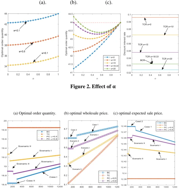
Then, numerical experiments show the different effects of 𝛼 in Figure 2. We consider banks and manufacturers to have the same risk preference, which means that h=e=10 and give TC=1200. We find that order quantity increases in 𝛼, with different given wholesale prices in (a). Order quantity decreases in wholesale price the same as to the above result. We note that if the retailer undertakes more finance from the bank, he may improve his order quantity when the wholesale price is the same. In this case, the bank discount interest rate is 0.032, and the trade credit discount interest rate is 0.072. What about the situation where trade credit has a lower cost? We consider different manufacturer risk preference levels in (b) and interest rate in (c) to explore if the result will change.
[Please insert Figure 2 about here]
We conclude that q increases with the ratio of bank credit when the manufacturer's risk preference is under a threshold. Nevertheless, when risk preference level exceeds the
threshold, as a result of the interest rate decreasing, the order quantity decreases first and then increases with 𝛼. For a given 𝛼, quantity increases in e. We find that if e=18.33, the order quantity by bank credit and trade credit is the same. Moreover, banks and manufacturers offer the same discount rate for the retailer. When e exceeds this threshold, the trade credit is more efficient.
6.1.2 Scenario II
For this situation, the retailer's repayment to the bank consisting of two parts. Within the credit line's part, the retailer needs to pay the bank for 𝑔𝑇𝐶(1 + 𝑟𝐶,𝐵). For another
part of the loan, it needs to pay (𝐿𝐵− 𝑔𝑇𝐶)(1 + 𝑟𝐵). The repayment to trade credit is 𝐿𝑇(1 + 𝑟𝑀). Similar to Equation (21), the expected profit function of the retailer in this scenario could be expressed as:
𝜋𝑟,𝑃,𝐼𝐼 = 𝐸(𝑝)𝑞 − (𝐸(𝑝) − 𝑠) ∫ 𝐹(𝑥)𝑑𝑥 𝑞
0 − 𝑔𝑇𝐶(1 + 𝑟𝐶,𝐵) − (𝐿𝐵− 𝑔𝑇𝐶)(1 + 𝑟𝐵) −
𝐿𝑇(1 + 𝑟𝑀) − 𝑇. (25)
It can be expressed as follows when we substitute 𝐿𝐵, 𝐿𝑆, and 𝑟𝐶,𝐵.
𝜋𝑟,𝑃,𝐼𝐼 = 𝐸(𝑝)𝑞 − (𝐸(𝑝) − 𝑠) ∫ 𝐹(𝑥)𝑑𝑥 𝑞
0 − 𝑔𝑇𝐶(1 + 𝑟𝐵− 𝑔𝑢ℎ𝑇𝐶) − (𝛼(𝑤𝑞 − 𝑇) −
𝑔𝑇𝐶)(1 + 𝑟𝐵) − (1 − 𝛼)(𝑤𝑞 − 𝑇)(1 + 𝑟𝑀) − 𝑇. (26)
Lemma 2. There is no optimal ratio for the retailer to decide. When 𝑟𝑀 > 𝑟𝐵, the retailer's profit increases in 𝛼; When 𝑟𝑀 < 𝑟𝐵, the retailer's profit decreases in 𝛼.
Considering a given 𝛼, we study the management decision by the retailer. Proposition 8 is given.
Proposition 8. In a decentralized supply chain, the retailer is given preferential credit
and finances by bank credit and trade credit portfolio. When the bank loan is higher than the credit line, the optimal order quantity satisfies the first-order optimality condition of its expected profit, which is given as follows:
𝑎 − 2𝑏 ∫𝑞𝑃,𝐼𝐼∗ 𝐹̅(𝐷)𝑑𝐷
0 − 𝑠 =
𝑤(1+𝑟𝑀+𝛼(𝑟𝐵−𝑟𝑀))−s
𝐹̅(𝑞𝑃,𝐼𝐼∗ ) . (27)
Equation (27) give the optimal order quantity when retailers use trade credit and bank credit simultaneously in the condition of that bank loan is higher than credit line. It shows that the optimal order quantity in scenario II is affected by 𝑟𝑀, 𝑟𝐵, and 𝛼. There is no effect of collateral and risk preference.
Corollary 5. (Effect of 𝜶) In scenario II, optimal order quantity increases in 𝛼,𝜕𝑞𝑃,𝐼𝐼
∗
𝜕𝛼 >
This Corollary shows the effect of bank financing ratio, trade credit interest rate and
bank interest rate on order decision. With high cost of financing, order quantity decreases.
6.2. Manufacturer’s problem
At the end of the selling period, manufacturer will receive extra interest revenue with 𝐿𝑇𝑟𝐶,𝑀 in scenario I and 𝐿𝑇𝑟𝑀 in scenario II. Thus, based on Equation (13), we obtain the manufacturer’s profit function as follows:
𝜋𝑚,𝑃,𝐼 = (𝑤 − 𝑘)𝑞 + 𝐿𝑇𝑟𝐶,𝑀. Scenario I
𝜋𝑚,𝑃,𝐼𝐼 = (𝑤 − 𝑘)𝑞 + 𝐿𝑇𝑟𝑀. Scenario II (28) When we substitute 𝐿𝑇, 𝑟𝐶,𝑀 into Equation (28), it could be written as:
𝜋𝑚,𝑃,𝐼= (𝑤 − 𝑘)𝑞 + (1 − 𝛼)(𝑤𝑞 − 𝑇)(𝑟𝑀− 𝑒𝑢 × (𝑔𝑇𝐶 − 𝛼(𝑤𝑞 − 𝑇))). Scenario I
𝜋𝑚,𝑃,𝐼𝐼= (𝑤 − 𝑘)𝑞 + (1 − 𝛼)(𝑤𝑞 − 𝑇)𝑟𝑀. Scenario II (29)
The Equation (29) represents the manufacturers’ profit in Scenario I and Scenario II when retailers finance inventory from the portfolio of bank loan and trade credit. It also helps to identify the optimal manufacturers’ operational decision. The manufacturer’s optimal wholesale price in two scenarios can be given respectively in Equation (30) and Equation (31).
Proposition 9. In a decentralized supply chain, the retailer receives preferential credit
from the bank and finances by bank credit and trade credit portfolio. The wholesale price in Scenario I (𝑤𝑃,𝐼∗ ) and Scenario II (𝑤𝑃,𝐼𝐼∗ ) are uniquely given by the following:
(i) In scenario I, 𝑤𝑃,𝐼∗ satisfies
𝑞𝑃,𝐼∗ (1 + 𝑟𝐶,𝑀(1 − 𝛼) + 𝛼𝑒𝑢𝐿𝑇) + 𝛼(1+𝑟𝐶,𝐵)+(1−𝛼)(1+𝑟𝐶,𝑀)+𝛼𝑒𝑢𝐿𝑇+2𝑒𝛼𝑤𝑢(1−𝛼)𝑞𝑃,𝐼∗ 𝑓(𝑞𝑃,𝐼∗ )(2𝑏 ∫𝑞𝑇∗𝐹̅(𝐷)𝑑𝐷 0 −𝑎+𝑠)−2𝑏𝐹̅(𝑞𝑃,𝐼∗ ) 2 −2𝛼𝑢𝑒(1−𝛼)𝑤2(𝑤(1 + 𝑟𝐶,𝑀(1 − 𝛼) + 𝛼𝑒𝑢𝐿𝑇) − 𝑘) = 0. (30)
(ii) In scenario II, 𝑤𝑃,𝐼𝐼∗ satisfies 𝑞𝑃,𝐼𝐼∗ (1 + 𝑟𝑀(1 − 𝛼)) + 1+𝑟𝑀+𝛼(𝑟𝐵−𝑟𝑀) ℎ(𝑞𝑃,𝐼𝐼∗ )[𝑠−𝑤(1+𝑟 𝑀+𝛼(𝑟𝐵−𝑟𝑀))]−2𝑏𝐹̅(𝑞𝑃,𝐼𝐼∗ ) 2(𝑤(1 + 𝑟𝑀(1 − 𝛼)) − 𝑘) = 0. (31) Where𝑞𝑃,𝐼∗ = 𝑇 𝑤+ 𝐹̅(𝑞𝑃,𝐼∗ )(𝑎−2𝑏 ∫0𝑞𝑇∗𝐹̅(𝐷)𝑑𝐷−𝑠)+𝑠−𝛼𝑤(1+𝑟𝐵−𝑔𝑢ℎ𝑇𝐶)−𝑤(1−𝛼)(1+𝑟𝑀−𝑒𝑢𝑔𝑇𝐶) 2𝑤2𝛼(1−𝛼)𝑒𝑢 . and 𝑎 − 2𝑏 ∫𝑞𝑃,𝐼𝐼∗ 𝐹̅(𝐷)𝑑𝐷 0 − 𝑠 = 𝑤(1+𝑟𝑀+𝛼(𝑟𝐵−𝑟𝑀))−s 𝐹̅(𝑞𝑃,𝐼𝐼∗ ) .
Proposition 9 reveals that when the retailer sources both with bank credit and trade credit, called portfolio credit, there is a different effect of risk preference and interest rate on wholesale price according to scenario I and scenario II.
7. Managerial implications
In this section, numerical experiments are given to explore the operational decision in the decentralized supply chain. Due to the fact that the detailed data of trade credit contract is non-publicize, especially about the SMEs. It is hard to test the impact of preferential credit on supply chain decision with empirical distributions. In fact, many researches always consider the numerical experiments with stochastic demand distribution to exam the result (Kouvelis and Zhao, 2012; Yang and Birge, 2018; Wu et al., 2019). We assume that the demands are uniform distribution, with D~U (0, 100) and give other parameters as follows: a = 14, b = 0.09, 𝑟𝐵= 0.08, s = 2, g = 0.4, k= 5, T = 50.
Under the condition of a decentralized supply chain, the retailer and the manufacturer decide the order quantity and wholesale price based on maximizing profit, respectively. We study the management decision and firms' profit, considering the retailer's collateral and different discount rate loan, which is given by bank (BC), manufacturer (TC), and portfolio credit (PC).
7.1 Effect of bank risk preference level
The bank risk preference level (h) would affluence the discount bank interest rate in BC and PC, and in turn, it can change the decision by retailer. We summarize the effect of bank risk preference on optimal order quantity, wholesale price, expected sale price, retailer's profit, manufacturer's profit, and the supply chain profit with bank credit and portfolio credit in Table 2.
For bank credit, under the conditions of case 1, bank risk preference has a positive effect on the order quantity and wholesale price but leads to a decrease in expected sale price. The retailer’s profit, manufacturer, and supply chain profit increase with bank risk preference. Under the conditions of case 2, order quantity, wholesale price, and expected sale price are not be affected by bank risk preference. Moreover, the manufacturer's profit is not influenced by bank risk preference. Nevertheless, the rise of banks' risk preference levels will promote the profit of the retailer and the supply chain.
[Please insert Table 2 about here]
When we consider portfolio credit, for the scenario I, the bank risk preference has a similar effect on management decisions of retailer and manufacturer to bank credit of
case 1. The retailer, manufacturer, and supply chain profit all increase with bank risk preference. As to scenario II, bank risk preference's effect on operational decision is similar to bank credit of case 2.
7.2 Effect of manufacturer risk preference level
We investigate the effect of manufacturer risk preference level under trade credit and portfolio credit and analyze the results in this subsection. The result is showed in Table 3.
[Please insert Table 3 about here]
As seen from Table 3, considering trade credit, we conclude that the manufacturer's risk preference has no effect on order decision and expected sale price. However, this can improve the wholesale price given by the manufacturer. A higher risk preference manufacturer offers trade credit to the retailer, leading to dwindling in the retailer's profit. The manufacturer's profit increases with her risk preference. The supply chain profit will not change with the manufacturer's risk preference.
Considering portfolio credit, under conditions of scenario I, we learn that the order quantity decreases with the manufacturer's risk preference. This result has a positive effect on wholesale price and expected sale price. With the rise in the manufacturer's risk preferences, both retailer and supply chain profit decrease. Manufacturer’s profit increases. In scenario II, because there is no preferential trade credit, the manufacturer's risk preference has no effect on operational decisions.
7.3 Effect of collateral
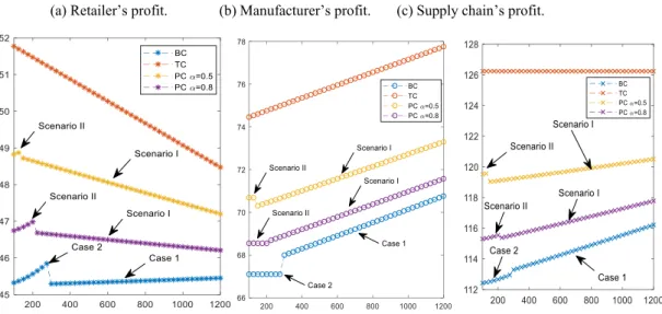
The effect of the retailer's collateral will be illustrated in this subsection. We set different ratios of bank credit (𝛼 = 0.5andα = 0.8) in portfolio credit conditions. The bank risk preference (h) amounts to 5, and the manufacturer risk preference (e) is 15. We compare different finance methods with collateral change.
[Please insert Figure 3 about here]
As can be seen in Figure 3(a), the optimal order quantity increases in retailer's collateral under BC and PC condition. The quantity may not change under TC. However, the order quantity under TC is the highest than the others. For PC conditions, with the increasing ratio of bank credit, the retailer will order less quantity from the manufacturer. Figure
3(b) shows the different effects of collateral on wholesale price. The wholesale price increases dramatically with the retailer's collateral under trade credit. For other financing methods, the wholesale price charged by the manufacturer increases slightly. With the increase in 𝛼, wholesale price rises. For trade credit conditions, the wholesale price is the lowest, and it is highest in bank credit conditions. The sale price is shown in Figure 3(c). Under TC, the sale price is the lowest with no change as collateral changing. For other financing methods, sale price decreases in collateral. With the increasing of 𝛼, sale price increases. Of interest, for bank credit in case 2 and portfolio credit in scenario II, the order quantity, wholesale price, and sale price will not change with the retailer's collateral.
[Please insert Figure 4 about here]
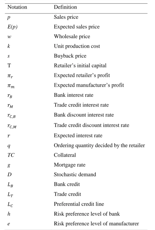
From Figure 4, we infer that the retailer that owes more collateral may not increase his profit with preferential credit. The discount interest rate may transfer to the manufacturer by pay for higher-order product expenses. However, the total supply chain profit will increase with collateral. As we have seen in Figure 4(a), the retailer's profit in TC financing conditions is higher than the others, although it decreases sharply with collateral. Under bank credit conditions, the retailer's profit increases slightly in case 1 but increases dramatically in case 2. The profit in case 2 is higher than that in case 1. Further, the retailer's profit under PC condition is located between those under BC and TC conditions. With the increasing of 𝛼, the profit will decrease. From Figure 4(b), the manufacturer has the highest profit under TC and gains the lowest profit under BC. The profit of the manufacturer is increasing with collateral under all financing methods. For supply chain profit, as seen in Figure 4(c), the collateral has no effect on that under trade credit. By trade credit, the supply chain has the highest profit than others. For bank credit and portfolio credit, the supply chain profit increases with the retailer's collateral. Furthermore, under bank credit conditions, the profit of the supply chain is the lowest.
We further discuss the other effects of the retailer's collateral on financing. Figure 5 gives collateral's influences to the expected interest rate, total interest, and total loan of retailers. It is crucial for us to explore the impacts of preferential credit from banks on management decisions.
[Please insert Figure 5 about here]
From Figure 5, we find that the expected rate of different financing methods decreases in collateral. The interest rate in trade credit is initially the highest. We conclude that
although the trade credit owes the highest financing unit cost and needs to be paid the highest interest, the retailer financing by trade credit would be the most profitable. In this way, trade credit is better than bank credit. We propose that the retailer’s decision needs to focus on choosing financing methods rather than only considering the interest rate and discount. The benefits of a discount loan interest rate may ultimately transfer to the manufacturer.
8. Conclusion
In this paper, we examine the effect of preferential credit on management decisions for capital-constraint retailers. In the competitive market, the bank offers preferential credit for high-quality retailers with collateral. The manufacturer also offers trade credit of discount interest rate based on the retailer’s credit line, which is evaluated by the bank. The bank risk preference and manufacturer risk preference may affect the discount interest rate of credit. The effect of preferential credit primarily depends on the retailer's collateral and financing institute’s risk preference. We investigate which financing methods would be the best for the retailer to finance, Bank credit, trade credit, or financing from both banks and manufacturers. Depending upon the loan amount compared to the credit line, financing in bank credit has two cases, and portfolio credit also has two scenarios in our model based on the relationship between credit line and bank loan. We model different situations to investigate operational decisions. Furthermore, a quantity-discount contract to coordinate the supply chain is considered in our model.
We find that with increasing bank risk preference levels, the retailer’s optimal order quantity will increase from bank credit due to the decreasing of financing cost. The retailer’s profit will increase in both case 1 or case 2. Both the wholesale price and manufacturer’s profit increase with bank risk preference level. The retailer’s collateral has a positive effect on supply chain decisions. However, under trade credit, the manufacturer’s risk preference level does not affect order strategies and retailer profit greatly. It can only improve the wholesale price and make the manufacturer's profit growth. The benefit that transfers to the manufacturer leads to harm to the retailer’s profit. There are no differences in the total supply chain profit. The retailer’s collateral will lead to a decreasing of the retailer's profit. But the total supply chain will increase. For portfolio credit, with the increasing of manufacturer risk preference, the retailer may order less, and the profit will be down when the part of bank loan
exceeds the preferential credit line. Moreover, collateral has a negative to the retailer’s decision. More collateral may not provide much profit directly to the retailer. There is no such effect in scenario I of risk preference and collateral. Consider different financing methods, and the trade credit is the most amicable for the retailer even though the financing cost is the highest.
In this paper, we investigate the effects of bank credit and trade credit under preferential credit situations in supply chain management. There are some attractive further research opportunities, including (i) credit finance with multiple manufacturers; (ii) dual-channel supply chain situations; (iii) trade credit from asymmetric manufacturers with competition. In the future, we would consider to investigate the impact of preferential credit from asymmetric manufacturers with competition on capital-constrained retailers. We hope this paper can guide the future management of capital-constrained supply chains from the perspective of real-world managers.
References
[1]. Breza, E., Liberman, A., 2013. The effect of trade credit on product markets: evidence from the suppliers of a large supermarket.
[2]. Burkart, M., Ellingsen, T., 2004. In-Kind Finance: A Theory of Trade Credit. American Economic Review 94, 569-590.
[3]. Carnovale, S., Rogers, D., and Yeniyurt, S., 2019. Broadening the Perspective of Supply Chain Finance: The Performance Impacts of Network Power and Cohesion. Journal of Purchasing and Supply Management 25 (2): 134–145. doi:10.1016/j.pursup.2018.07.007.
[4]. Chen, J., Zhou, Y.-W., Zhong, Y., 2017. A pricing/ordering model for a dyadic supply chain with buyback guarantee financing and fairness concerns. International Journal of Production Research 55, 5287-5304
[5]. Chod, J., 2016. Inventory, Risk Shifting, and Trade Credit. Management Science 63, 3207-3225.
[6]. Chod, J., Lyandres, E., Yang, S.A., 2019. Trade credit and supplier competition. Journal of Financial Economics 131, 484-505.
[7]. Choi, T.-M., Li, D., Yan, H., Chiu, C.-H., 2008. Channel coordination in supply chains with agents having mean-variance objectives. Omega 36, 565-576.
[8]. Dada, M., Hu, Q., 2008. Financing newsvendor inventory. Operations Research Letters 36, 569-573.
[9]. Deng, S., Gu, C., Cai, G., Li, Y., 2018. Financing Multiple Heterogeneous Suppliers in Assembly Systems: Buyer Finance vs. Bank Finance. Manufacturing & Service Operations Management 20, 53-69.
[10]. Doumpos, M., Zopounidis, C., 2011. A Multicriteria Outranking Modeling Approach for Credit Rating. Decision Sciences 42, 721-742.
[11]. Emery, G.W., 1984. A Pure Financial Explanation for Trade Credit. Journal of Financial and Quantitative Analysis 19, 271-285.
[12]. Feess, E., Thuyn, J.-H., 2014. Surplus division and investment incentives in supply chains: A biform-game analysis. European Journal of Operational Research 234, 763-773.
[13]. Fisman, R., Love, I., 2003. Trade Credit, Financial Intermediary Development, and Industry Growth. The Journal of Finance 58(1), 353-374.
[14]. Gallego, G., van Ryzin, G., 1994. Optimal Dynamic Pricing of Inventories with Stochastic Demand over Finite Horizons. Management Science 40, 999-1020. [15]. Gao, G.-X., Fan, Z.-P., Fang, X., Lim, Y.F., 2018. Optimal Stackelberg strategies
for financing a supply chain through online peer-to-peer lending. European Journal of Operational Research 267, 585-597.
[16]. Granot, D., Yin, S., 2005. On the effectiveness of returns policies in the price-dependent newsvendor model. Naval Research Logistics (NRL) 52, 765-779. [17]. Gan, X., Sethi, S.P., Yan, H., 2005. Channel Coordination with a Risk-Neutral
Supplier and a Downside-Risk-Averse Retailer. Production and Operations Management 14, 80-89.
[18]. Gupta, D. 2008. Technical note: Financing the newsvendor. Working paper,
[19]. Gupta, S., Dutta, K., 2011. Modeling of financial supply chain. European Journal of Operational Research 211, 47-56.
[20]. Hu, X., Su, P., 2018. The newsvendor's joint procurement and pricing problem under price-sensitive stochastic demand and purchase price uncertainty. Omega 79, 81-90.
[21]. Huang, J., Yang, W., Tu, Y., 2019. Supplier credit guarantee loan in supply chain with financial constraint and bargaining. International Journal of Production Research, 1-16
[22]. Jacobson, T., von Schedvin, E., 2015. Trade Credit and the Propagation of Corporate Failure: An Empirical Analysis. Econometrica 83, 1315-1371.
[23]. Jammernegg, W., Kischka, P., 2013. The price-setting newsvendor with service and loss constraints. Omega 41, 326-335.
[24]. Klapper, L., Laeven, L., Rajan, R., 2011. Trade Credit Contracts. The Review of Financial Studies 25, 838-867.
[25]. Kouvelis, P., Zhao, W., 2011. The Newsvendor Problem and Price-Only Contract When Bankruptcy Costs Exist. Production and Operations Management 20, 921- 936.
[26]. Kouvelis, P., Zhao, W., 2012. Financing the Newsvendor: Supplier vs. Bank, and the Structure of Optimal Trade Credit Contracts. Operations Research 60, 566- 580. [27]. Kouvelis, P., Zhao, W., 2017. Who Should Finance the Supply Chain? Impact of Credit Ratings on Supply Chain Decisions. Manufacturing & Service Operations Management 20, 19-35.