HAL Id: hal-00111341
https://hal.archives-ouvertes.fr/hal-00111341
Submitted on 18 Mar 2021
HAL is a multi-disciplinary open access
archive for the deposit and dissemination of
sci-entific research documents, whether they are
pub-lished or not. The documents may come from
teaching and research institutions in France or
abroad, or from public or private research centers.
L’archive ouverte pluridisciplinaire HAL, est
destinée au dépôt et à la diffusion de documents
scientifiques de niveau recherche, publiés ou non,
émanant des établissements d’enseignement et de
recherche français ou étrangers, des laboratoires
publics ou privés.
Distributed under a Creative Commons Attribution| 4.0 International License
Experimental and numerical analysis of localization
during sequential test for an IF-Ti steel
Thierry Hoc, Collette Rey, Jean Raphanel
To cite this version:
Thierry Hoc, Collette Rey, Jean Raphanel. Experimental and numerical analysis of localization during
sequential test for an IF-Ti steel. Acta Materialia, Elsevier, 2001, 49, pp.1835-1846.
�10.1016/S1359-6454(01)00076-3�. �hal-00111341�
EXPERIMENTAL AND NUMERICAL ANALYSIS OF
LOCALIZATION DURING SEQUENTIAL TEST FOR AN IF–Ti
STEEL
T. HOC1†, C. REY1and J. L. RAPHANEL2
1Laboratoire de Me´canique des Sols, Structures et Mate´riaux, Ecole Centrale Paris, UMR 8579, Grande Voie des Vignes, 92295 Chaˆtenay-Malabry Cedex, France and2Laboratoire de Me´canique des Solides,
Ecole Polytechnique, CNRS-UMR 7649, 91128 Palaiseau Cedex, France
Abstract — Localization of plastic deformation in polycrystals often occurs after a change of loading path. An
experimental study using several techniques at different scales (scanning electron microscopy, microgrids, local orientation measurements, transmission electron microscopy) has been conducted on mild steel sheets (interstitial free titanium steel) prestrained by plane tension and then deformed by uniaxial tension along the first tensile axis or the transverse axis. In this way localization has been linked to microstructural anisotropy developed during the first loading path. A model based on crystalline plasticity has then been introduced in a finite element code (Abaqus) with a description of intragranular hardening linked to the evolution of the dislocation densities on each slip system. The simulations make use of a finite element representative pattern based on actual grain distribution in the aggregate. The computations predict a localization in good agreement with the experimental data and show a link between saturation of dislocation densities and concentration of plastic deformation.
Résumé — La localisation de la déformation plastique dans les polycristaux peut apparaître lors de
changements de trajets de chargements. Une étude expérimentale utilisant plusieurs techniques à différentes échelles (microscopie électronique à balayage, microextensométrie, mesures locales d’orientations, microscopie électronique à transmission) a été effectuée sur une tôle d’acier doux prédéformée en traction plane soumise à des essais de traction simple dans le sens de prédéformation ou dans la direction orthogonale. La localisation a alors été reliée à l’anisotropie microstructurale formée pendant le premier trajet. Un modèle cristallin basé sur l’évolution des densités de dislocations attachées à chaque système de glissement a été introduit dans le code élement finis Abaqus. Ce modèle utilisant un motif représentatif extrait de l’expérience a permis une simulation de la localisation en bon accord avec les résultats expérimentaux et a confirmé la relation entre la saturation de la densité de dislocation et la concentration de la déformation plastique.
Keywords:Steel; Microstructure; Mesostructure; Scanning electron microscopy (SEM); Finite element
1. INTRODUCTION
Forming processes of polycrystalline sheets are often hampered by strain localizations which lead to dam-age or rupture and strongly limit the metal for-mability. The material is subjected to large strains and an element of volume follows a complex loading path. Sequential loading paths have thus been exten-sively used to simulate the process and to gain some understanding of strain localization phenomena in polycrystals [1–3]. These studies have established that strain localizes within bands and have linked this behavior to two main sources of softening resulting
† To whom all correspondence should be addressed. Tel.: +33-1-4113-1616.
E-mail address:hoc@mssmat.ecp.fr (T. Hoc)
from the evolutions of crystallographic textures and intragranular microstructures [4]. The crystalline structure of the material and the physical mechanisms of plastic deformation by intragranular slip on parti-cular crystallographic slip systems have thus to be accounted for. Along a monotonic load path, there is both a reorientation of the grains to optimize the conditions of plastic slip and an intragranular arrange-ment of dislocations to form walls with a high dislo-cation density limiting cells of low dislodislo-cation den-sities. These orientations and structures will interact and evolve when a change of strain path is imposed. The use of finite element codes in crystalline plas-ticity has been growing rapidly in the past 15 years and three main applications can be found in the litera-ture. The first is devoted to single and bi-crystals under monotonic and cyclic loadings [5], the second uses crystalline behavior to predict the development
of deformation textures [6, 7] for polycrystalline aggregates, and the third is focused on the study of heterogeneous local (intra- and intergranular) strain and rotation fields [8–10] for special aggregates with a small number of grains or for an area of a real polycrystal. Most of these studies are based on a mon-otonic or at the most cyclic load path and do not take into account a pre-existing intragranular microstruc-ture. To the best of our knowledge very few simula-tions have been performed with the aim of studying the strain localization after a change of loading path. The main problem in this case arises in the simulation of the second path for which an adequate description has to be provided for the microstructural anisotropy and hardening resulting from the activation of slip systems during the first path.
The present work, which includes an experimental study and numerical simulations, is an attempt to evaluate the respective roles of the intragranular microstructure and the deformation texture on the strain localization for mild steel sheets submitted to a sequential loading path composed of plane strain followed by uniaxial tension.
The experimental study has focused on the analysis of the localization occurring at the beginning of the second loading path. The characterization of the material at the macroscopic scale is obtained by sev-eral mechanical experiments using uniaxial testing machines and by deformation texture measurements with a texture goniometer. Strain localization during the second loading path is analyzed at the scale of the grains via in situ mechanical testing performed by scanning electron microscopy (SEM) with local orientation measurements with electron back-scat-tered diffraction (EBSD) and local strain measure-ment with microgrids deposited on the surface of the polished sample. At the smaller scale of the dislo-cation microstructures, thin foils are observed by transmission electron microscopy (TEM) to charac-terize dislocation cells (shape, orientation, etc.).
A crystalline model for plasticity and hardening is then proposed and introduced in the Abaqus finite element code. It allows us to simulate the evolution of the local strain field and the density of dislocations on the different slip systems before and at the begin-ning of the localization during the second loading path. One originality of the simulations is to build a virtual aggregate by the juxtaposition of an actual pat-tern of 114 grains called hereafter the “finite element
representative pattern” (FERP) whose initial
geometry, i.e. grain shape and size, position of grain boundaries and initial crystallographic orientations, has been measured on an area of the actual polycrys-tal.
Experiments and simulations are shown to be in reasonable qualitative agreement. The simulations provide estimates of non-directly measurable quan-tities such as dislocation densities or glide magnitudes which contribute to the analysis of experimental data.
2. EXPERIMENTAL PROCEDURE
The material and the experimental procedure have been described elsewhere [11]. In order to make this paper self-contained, we recall only some key elements in this section. The mild steel sheets (0.9 mm thick) have been initially cold-rolled, then annealed and skin-passed so that the initial crystallo-graphic texture is close to a ⬍111> fiber texture. The average grain size is 20 µm.
The first load path is plane strain along the rolling direction (RD) up to macroscopic logarithmic strain values of about 0.12, 0.18 and 0.24; these three prede-formed states are denoted by ⑀=0.12, ⑀=0.18 and ⑀=0.24 respectively. The second load path is uniaxial tension. It is applied to smaller samples taken from a region of uniform prestrain (checked by measures on a 1 mm×1 mm grid) with their tensile axis parallel or orthogonal to the RD [12]. A letter L or T respect-ively is used to denote this second loading path. These tensile tests are performed by SEM at 353 K, and are referred as in situ tests [13].
Microgrids (area 1 mm2; mesh 5 µm×5 µm) have
been deposited on the surface of the polished samples. The measure of the three-dimensional positions of their nodes in the initial and deformed states allows the computation of six components of the transform-ation gradient tensor F
˜ (namely F11, F12, F21, F22, F31,
and F32) between two successive configurations at
time t and t+dt (reference and current configurations respectively). The component F33can be estimated by the conservation of volume, but F13and F23cannot be determined by surface measurements. Three components of the Green–Lagrange tensor E
˜ (namely
E11, E12and E22) are then computed in the reference configuration. With the assumption of linearity between two successive steps, one can estimate components of the velocity gradient L
˜, hence
compo-nents of the deformation and rotation rates. More details on the technique and computation can be found in [14–16]. During the same test, the local orientations of several grains were measured using the EBSD technique.
In order to characterize heterogeneities at a smaller scale, some transmission electron microscopy (TEM) observations were carried out after the prestrain and after the second load path. These observations of dis-location cells were performed at 200 kV with a JEOL 200CX electron microscope equipped with a double tilt goniometer. The preparation of the samples required mechanical polishing to a thickness of approximately 150 µm followed by final thinning by a twin-jet electropolisher with an electrolyte com-posed of 5% perchloric acid in 2-butoxyethanol sol-ution at 55 V and 12°C. Light marks were engraved on the sample edges parallel to the RD direction.
3. CRYSTAL PLASTICITY MODEL
A crystalline plasticity constitutive model that accounts for deformation by crystallographic slip and
for lattice rotation with deformation was used in this analysis and implemented in the Abaqus finite element code. Implementations of the constitutive relations as a User Material subroutine in the Abaqus code have been described by Smelser and Becker [17]. The mechanical modeling follows the frame-work developed by Peirce et al. [18] and used later by Teodosiu et al. [19].
The kinetics of large transformations are used which are based on the multiplicative decomposition of the deformation gradient into elastic and plastic parts. The velocity gradient L
˜ is decomposed
addi-tively into an elastic part L
˜
eand a plastic part L
˜
pdue to glide on crystallographic slip systems. A system (s) is defined by a glide direction g→(s) and a glide plane normal n→(s). For body-centered cubic (b.c.c.) materials such as α-iron, the directions are the ⬍111> directions and we consider glide on the {110} and {112} planes which lead to 24 slip systems [20, 21]. The kinetics can be summed up by the following equations: L ˜= D˜ + W˜ = L˜ e+
冘
s g˙(s)→(s)g 丢 n→(s) (1) where D˜ and W˜ are respectively symmetric and
anti-symmetric parts of L
˜ and g˙
(s)is the slip rate on sys-tem (s).
The rate form of the constitutive equation couples elastic behavior with the flow theory of plasticity in the following way:
t 왓 苲 = K ⬇:D˜ ⫺
冘
s g ˙(s)R ˜ (s) (2) where t왓 苲is the Jaumann rate of Kirchhoff stress, defined by t 왓 苲 = t· 苲 ⫺W ˜t˜+ t˜W˜ (3) K
⬇strains identifies with the usual fourth rank tensor ofis a tensor of elastic moduli, which for small elastic elastic moduli c
⬇and R˜
(s) is a tensor containing the slip geometry and may be expressed as:
R ˜ (s)= K ⬇:D˜ (s)+ W ˜ (s) t ˜⫺t˜W˜ (s) (4)
The plastic slip rates are determined by a viscoplastic power law with the introduction of a threshold, so that the activation of a slip system (s) is governed by Schmid’s law, |ts|ⱖts
c where tsc is the critical shear stress, which depends on the structural variables and temperature, while ts is the resolved shear stress on slip system (s) given by ts= s˜:( ›
gs丢 n→s). The viscoplastic law gives:
g ˙s= g˙ o
|
ts tsc|
n sgn(ts) if |ts|>ts c g ˙s=0 otherwise (5)where g˙ois a reference strain rate, the exponent n is close to 100 at room temperature for metallic materials.
Hardening characteristics of the material depend on the interaction mechanisms between the different slip systems (activated and latent slip systems) at the con-sidered temperature and strain rates. Hardening is governed by the stacking fault energy of the metal, the density of dislocations, and the mean free path of the activated dislocations. It is generally expressed by
a hardening matrix whose components hsu take into
account the interactions between systems (s) and (u):
t˙sc=
冘
uhsu|g˙u| (6)
In its simplest form, the hardening matrix is taken with constant coefficients, sometimes reduced to two values, one for diagonal terms expressing self-harden-ing and one for off-diagonal terms or latent hardenself-harden-ing terms. This can hardly be the case for sequential tests, where latent slip systems during the first loading become activated slip systems during the second path. It is thus important to express the coefficients of the hardening matrix in terms of internal variables whose evolutions may be linked to the history of plastic deformation in the material. In our case we chose to use an average dislocation density on each slip sys-tem.
The evolution of the total dislocation density, based on Orowan’s relation and an annihilation process of dislocation dipoles [22], is given by:
r˙s=1
b
冉
1
Ls⫺Gcrs
冊
|g˙s| (7)where b is the magnitude of the Burgers vector, Gc
a parameter proportional to the characteristic length associated with the annihilation process of dislocation dipoles, and Lsthe mean free path of system (s) which can be expressed by:
Ls= K
冉
冘
u⫽sru
冊
⫺1/2(8)
where ruis the total dislocation density on a latent system (u). In this formulation, K is a material para-meter and the dislocation–dislocation interactions (forest interactions) are the only ones taken into account.
The critical shear stress on system (s) can be related to the dislocation densities by the relation:
Table 1. Parameters of the model a0 K t0(MPa) Gc(nm) n g˙0(s⫺1) r0(m⫺2) k1 k2 kp1 kp2 ks0 0.2 20 22 10 99 0.8×10⫺15 66×109 1 1.15 1.05 1.05 1.3 tsc= to+ mb
冉
冘
u asu ru冊
1/2 (9) where tois the friction stress which depends ontem-perature and asu characterizes the interactions
between two families of dislocations (s) and (u). By differentiation of equation (9) with respect to time, the phenomenological law (6) is obtained and the hardening matrix [23] is now given by:
hsu=m 2a su
冉
冘
l asl rl冊
⫺1/2冦
1 K冉
冘
l⫽u rl冊
1/2 ⫺G cru冧
(10) The hardening matrix depends explicitly on the cur-rent values of the dislocation densities. Its form is similar to the one suggested by Franciosi [24, 25] for b.c.c. single crystals and small strains. In his model, the terms hsu increase with the strain amplitude and present a sharp variation at the beginning of the plas-tic deformation, then tend to a constant.In order to determine the different parameters of the hardening law, a polycrystalline self-consistent model using an explicit concentration law has been developed. The identification of the physical para-meters is performed via an inverse method by using different loading paths including uniaxial tension, plane strain, cyclic plane shear and plane strain tests followed by uniaxial tensile tests. The homogeneous parts of the responses are the only parts used for identification purposes. The macroscopic stresses and texture evolutions are computed and compared to experimental results. Details of the procedure are given in [26]. The hardening law parameters obtained by this approach have values in good agreement with literature. These values are given in Table 1 where
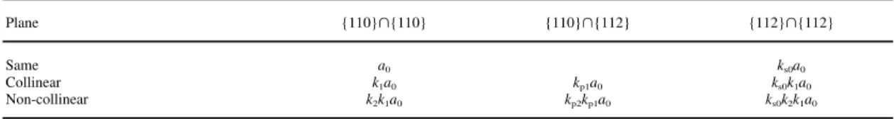
a0, k1, k2, kp1, kp2and ks0 are interaction coefficients between families of dislocations (as defined in Table 2).
The relations outlined above require a very small time step to achieve stable and accurate numerical integration. This is mainly due to the highly
non-lin-Table 2. Interaction coefficients
Plane {110}傽{110} {110}傽{112} {112}傽{112}
Same a0 ks0a0
Collinear k1a0 kp1a0 ks0k1a0
Non-collinear k2k1a0 kp2kp1a0 ks0k2k1a0
ear nature of the viscoplastic power law used for the computation of the slip rates. In order to increase the time step size, a forward gradient method has been used [27] for the integration of slip rates.
4. EXPERIMENTAL RESULTS
4.1. Macroscopic strain localization
Figure 1 shows typical nominal stress–stretch curves for the prestrained samples tested in tension along the rolling direction (L) and the transverse direction (T). The stretch is given by the ratio of the cross-head displacement to a gauge length Lo.
The virgin material presents the same behavior in uniaxial tension along the rolling or the transverse direction. The effect of a prestrain by plane strain is to increase the yield stress and to produce a very specific shape of the reloading curves which can be divided into three distinct stages (after a short initial transition at the very start of the loading):
1. an elasto-plastic transition which extends to about 1% and is parabolic in the transverse direction and sharper in the rolling direction;
2. a sudden load decrease more pronounced in the transverse direction;
3. a linear decrease of the load with stretch. Analysis of the nominal stress–stretch curves can be made in connection with the surface observation of the macroscopic strain localization (Fig. 2). The maximum of the load corresponds to the onset of the macroscopic strain localization in a macroband at about 54° to the tensile axis irrespective of the tensile direction. A second symmetrical macroband (see Fig. 2) is activated for a small increase in the applied strain for all samples tested in the rolling direction and for the sample ⑀=0.12T. In the case of sample
⑀=0.18T a new symmetrical macroband is activated
at 5.7% of stretch and no new macroband occurs for the sample ⑀=0.24T.
The computation of the evolution of the strain and rotation fields within the macrobands during post-bifurcation is based on microextensometry with a step
Fig. 1. Nominal stress–stretch curves.
Fig. 2. Localization function of prestrain and reloading direction. The initial width of the sample is 3 mm.
of 50 µm. The measure is done along a line parallel to the tensile axis which intersects the macrobands. The origin is fixed somewhat arbitrarily at some dis-tance from the band. Figures 3a and b show respect-ively the distribution along that line of the values of
Fig. 3. Local strain and rotation fields: (a) local deformation E22; (b) local rotation W12(in degrees).
the axial strain E22and rotation angle W12for the sam-ple ⑀=0.12T at several stages of deformation along the new path, namely 4%, 5.7%, 8.2% and 10.6% of macroscopic strain. Since Lagrangian quantities are used, they are plotted on the initial undeformed
con-figuration, on a vertical at a given abscissa one finds the values for the same material point.
The axial component of strain E22 reaches fairly
large values within the band (larger than 1, for an average macroscopic strain of 10.6%) and is close to zero elsewhere. Figure 3a shows the propagation mechanism of the macrobands with, for each macrob-and, one front remaining fixed (the one near the fixed origin of our abscissa) and the other propagating. The total rotation is large within the band, with a maximum absolute value of about 30°. The shear component E12is non-zero but remains small, and this is also the case when the shear component is expressed in a reference frame linked to the band [11].
4.2. Texture evolution and local orientations: the mesoscopic scale
Deformation texture measurements and compu-tations have been performed on virgin samples and after the prestrain. The initial texture is close to a fiber texture, with a ⬍111> fiber axis normal to the sheet plane. During plane strain a reinforcement of this fiber texture appears, increasing the average level of the orientation distribution function from 7 to 9. The textural evolution may thus be considered as somewhat limited.
Observations of the slip lines pattern within the macrobands (Fig. 4 of [11]) show two families of wavy (about 50 µm long) quasi-parallel coarse slip bands at ±50° from the tensile axis which appear at the beginning of the localization. We call these small parallel bands “mesobands”. This kind of mesostruc-ture is observed for all samples. With increasing deformation, the traces of these mesobands rotate towards the tensile axis.
This may be expressed in a more quantitative way by computing and plotting the distribution of the axial
component E22of the Green–Lagrange strain tensor.
The plot reflects the underlying structure of meso-bands (see Fig. 3 of [11]).
The local reorientation field is another interesting physical quantity which may be computed across the macrobands. The EBSD technique allows the
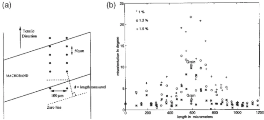
meas-Fig. 4. Local rotation in macroband for⑀=0.24T: (a) measurement procedure; (b) misorientation in macroband,
for stretches 1%, 1.3%, 1.5%.
ure of the local orientation of the same material point for several levels of straining along the second path. The orientation at the beginning of the appearance of the macroband is considered as reference (average macroscopic strain of 0.6% for ⑀=0.24T). The compu-tation of a reoriencompu-tation is made possible by using the Rodrigues vector as a metric representation of an orientation [28]. A difference between two Rodrigues vectors thus represents the local reorientation, which may be decomposed into an axis of rotation and an amplitude. In our case, it is ascertained that the reori-entation axes are very close to the sheet plane normal, so that only the amplitude needs to be plotted. Three successive levels of strain along the second path are considered (1%, 1.3% and 1.5%) and the material points are taken along two lines, parallel to the tensile axis and crossing the macroband. The principle of the measurement is shown in Fig. 4a. Figure 4b shows the magnitudes of the reorientation of the various material points. Note that the maximum value is near the middle of the band and that outside the band the reorientation is almost negligible. Inside the band the reorientation can vary greatly. For instance, the points labeled Grain A and Grain B in Fig. 4b have very different behaviors which cannot be due only to dif-ferent initial orientations. These points are located at the same distance from the origin axis, but are on two distinct lines of measurements (see Fig. 4a). The local behavior may thus be linked to the mesoband struc-ture, and may be attributed to different levels of axial strains.
4.3. Microscopic scale: evolution of the dislocation microstructures
TEM observations have been made in grains with a normal oriented along a ⬍111> direction which constitute the majority of the grains owing to the deformation texture. After a small amount of strain, dislocations tend to arrange themselves to form walls delimiting cells of material with low dislocation den-sities. The shape of these cells depends on the strain path. At the end of plane strain predeformation, the microstructure consists in two families of walls delimiting cells forming parallelograms.
Neverthe-less, a better definition of the set of walls at about 90° of the tensile axis is noted.
The microstructure of the sample ⑀=0.12T is stud-ied inside the macrobands during the second load path at 3% and 10% of macroscopic stretch. The micro-structure pattern at the smaller stretch level presents large fluctuations inside a grain and from grain to grain. Nevertheless, the dislocation arrangements typical of the preloading tend to disappear. For typical microstructure see, for instance, [29]. At the larger stretch level of 10%, the new dislocation cells have an aspect similar to cells which would have developed along the same strain path for a monotonic straining of virgin material.
5. NUMERICAL SIMULATIONS
The finite element code Abaqus was used, in which a constitutive model was introduced by means of a user subroutine UMAT. The model is based on physi-cal mechanisms of plastic deformation by intracrys-talline slip, for b.c.c. metals at a temperature slightly above the transition temperature (in our case the in situ experiments were at 353 K). Its equations have been given in Section 3, one only recalls here that it is a large-deformation, elasto-viscoplastic model with an original description of intragranular hardening. The coefficients of the hardening matrix are expressed in terms of dislocation densities on each slip system, which by their evolutions provide a model of the evolution of the anisotropy of the micro-structure in the course of a sequential loading. A satu-ration level has been introduced, since it has been observed that the large increase of deformation within a macroband does not give rise to a comparable increase of dislocation densities.
5.1. Finite element representative pattern
The polycrystalline structure had to be somewhat idealized for the implementation of a finite element code. Between the impossibility of knowing and meshing a three-dimensional structure, without destroying it, and the complete arbitrariness of imagining a virtual aggregate, a median way has been chosen which is to use a part of an actual polycrystal for the definition of a pattern of grains and to build up the complete structure by repeating this pattern. We call this pattern the finite element representative pattern (FERP) and we present hereafter its definition and how we have established its representativity.
The FERP is constructed from the surface of a mild
steel sample. An area Seof 190 µm×90 µm is used
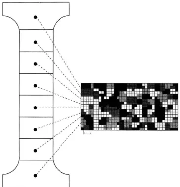
which contains 114 grains whose orientations are measured by EBSD. A grid of 5µm×5 µm is superim-posed which defines 684 elements, chosen as eight-noded brick elements. Each element is assigned a crystallographic orientation so that the grain bound-aries are followed approximately (see Fig. 5 where different shades of gray are used to visualize the dif-ferent grains).
A first check of the representativity of the FERP is that the crystallographic texture as measured by EBSD is close to the texture of the polycrystal, as measured by X-ray diffraction with a goniometer. The next check is by performing two simulations of a mechanical response, one using the FERP texture and the other with the complete experimental texture. The simulations of an uniaxial tensile test and of a cycle of plane shear deformation by a self-consistent model [26] using each data set show almost identical responses which supports the claim of representativity of the FERP.
In order to obtain a sample with adequate dimen-sions, the FERP is repeated eight times by translation along the tensile axis (see Fig. 5). The orientations of the 114 grains and the dislocation densities in each grain at the beginning of the second loading path cor-respond to the values computed at the end of the first loading. This method provides a direct construction of (T) samples. For (L) samples, we have chosen to keep the same morphology, that is to translate a FERP eight times along the tensile axis but to rotate each crystalline orientation by 90° about the normal to the sample surface. This avoids a tedious remeshing but has the drawback of introducing new orientation relations at the local level.
The results of computations presented hereafter only concern the simulation of the second loading path, that is, uniaxial tension along the rolling (L) or transverse (T) direction after a prestrain.
5.2. Stress–stretch curves
Figure 6 shows nominal stress–stretch curves in the transverse direction and in the rolling direction for any prestrain, as the result of a finite element compu-tation using the sample and mesh discussed above.
All these curves show an elasto-plastic transition and present a maximum followed by softening. Local-ization, which in a macroscopic sense may be equated with the maximum of a curve, occurs earlier for the L samples than for the T samples. For comparison, Fig. 6 shows the simulation by a self-consistent model [26] of a second path in tension along the transverse direction T of a sample with a 24% prestrain. The two models give very similar results in terms of elas-tic limit and maximum value (although the maximum is reached faster in the finite element simulation). The discussion will define the field of application of each type of approach.
Figure 6 retains the part of the curves, after the maximum nominal stress, which should be eliminated since the validity of the model in these cases can be questioned, not only for numerical stability reasons but also because the mechanisms of reorganizations of the dislocation substructures are not part of the model.
5.3. Local analysis
In order to compare the development of localiz-ation for (L) and (T) samples, the longitudinal strain
Fig. 5. Description of the finite element representative pattern (FERP).
Fig. 6. Nominal stress–stretch curves (self-consistent and finite element calculations).
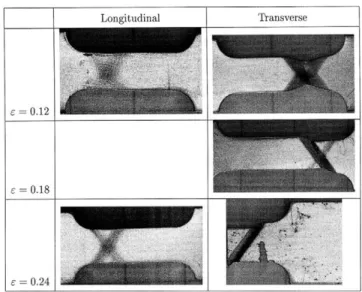
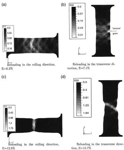
fields is examined at two successive steps of overall deformation for samples prestrained at ⑀=0.18. This analysis of the morphology of the localization process is one of the advantages of the finite element approach which computes the whole field of relevant mechanical quantities over the sample. At the begin-ning of the second loading, the deformation is mainly concentrated at the center of the (L) sample, while for sample (T) a large deformation occurs near the side of the sample. At a later stage, these two con-figurations develop localization bands presenting dif-ferent morphologies, diffuse necking for (L) and a well-defined macroband for (T). These results
corre-spond qualitatively to the experimental observations (Fig. 7).
A main advantage of the numerical simulations is to provide the local values of physical parameters inaccessible by experiments. More specifically, the glide quantities and the densities of dislocations can be computed in different grains. Before the beginning of the macroscopic localization and for all samples, the deformation is concentrated in five points forming a symmetrical configuration. For the reloading in the transverse direction (T) the evolution of this con-figuration is governed by the behavior of a “source” grain in which a large strain appears (see Fig. 7). On
Fig. 7. Longitudinal deformation obtained by finite element calculation for⑀=0.18L and⑀=0.18T. Reloading
in the rolling direction: (a) E=6.3%; (c) E=12.8%. Reloading in the transverse direction: (b) E=7.1%; (d)
E=15.7%.
the contrary, for the reloading in the same direction (L) this symmetrical configuration is rapidly erased and diffuse necking takes place. The local analysis of glide amplitudes and densities of dislocations in this grain is given in the figure for the case ⑀=0.18T.
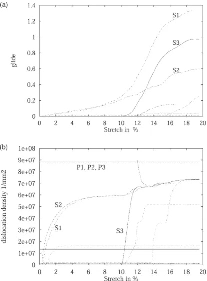
Figure 8a shows the initial activation of two sys-tems (S1,S2), then a sharp increase of the glide ampli-tude for one of the two slip systems previously acti-vated and the rapid activation of a new system (S3). This takes place at about 10% overall deformation and corresponds to a localization of the deformation. Figure 8b shows that the dislocation densities are constant on three slip systems (P1, P2, P3) close to 9×107 mm⫺2. This means that these three slip sys-tems, which have been activated during the first load-ing, are now latent. Deformation occurs by activation of two new slip systems whose dislocation densities
increase then saturate. Saturation close to 6×10⁷
mm⫺2
corresponds to localization. Note that the acti-vation of the third slip system is revealed by a very fast increase in its density of dislocation.
6. DISCUSSION
The phenomenon of localization and the behavior immediately following localization in prestrained
polycrystals subjected to a new loading path has been investigated experimentally at various scales. This experimental background has been the motivation for modeling the bifurcated behavior in a layer of grains which is obtained by the juxtaposition of an FERP with the texture and mechanical behavior similar to those of the whole polycrystal.
The objective of this modeling scheme is to account for the interactions between neighboring grains by using an actual grain distribution measured by EBSD. This provides a way to include second-order stresses in the model. At a smaller scale, the dislocation interactions are also included through the evolution laws for dislocation densities, validated in the transitory domain (beginning of a new loading path) and at the start of localization.
Our assumption is that localization results from the saturation, in terms of hardening capabilities or dislo-cation densities, of the active glide systems along the new loading path. This saturation is strongly influ-enced by the activity of glide systems during the first loading path which may have generated more or less strong obstacles to glide on the new systems. It is thus very important to have a model where intragranular anisotropy evolutions are well described. This is a reason for choosing a very anisotropic hardening
Fig. 8. Local parameters for the “source” grain (⑀=0.18T). (a) Glide quantities. (b) Dislocation density.
matrix with variable coefficients (see for instance [25]) and performing several experiments to validate the model. For b.c.c. metals it is necessary to consider 24 glide systems and the corresponding dislocation densities.
The finite element computations are consistent with the overall stress strain curves and they also repro-duce the main features of the bands of localization: diffuse localization for a longitudinal reloading (weak change of load path) and a well-defined band for a transverse reloading (strong change of load path).
The experimental analysis of the localization with a measure of local crystalline orientations within the macroband complements the one done by microexten-sometry and presented elsewhere [11]. The strain is mostly localized within macrobands which are made up of two conjugate families of mesobands that may probably be assimilated to coarse slip. The thickness of these bands is difficult to measure because of large strain gradients but it is almost of the order of the grain size. It seems that two families of glide systems, acting on planes more or less parallel across the grains, control the deformation immediately after
localization. EBSD measures made at material points inside and outside the bands show, in agreement with microextensometry measurements, that the macrob-ands present a fixed interface and an interface which moves as the deformation proceeds. This phenom-enon has also been observed in single crystals [16]. The propagation of a band takes place by activation of mesobands near the mobile interface. These meso-bands are the only sites of crystal rotations which may reach 30°. As strain and rotation saturate in a mesob-and, another one is activated. The strain level reached in the bands is very large and exceeds the scope of the constitutive laws which is why the numerical simulations should be limited to the beginning of post-bifurcation. It is also noteworthy that the axes of the bands rotate toward the tensile axis as the strain increases.
The activation of mesobands is accompanied by a macroscopic strain softening. This may be modeled by the evolution law for the densities of dislocations (recall Eq. (7)) whose parameters have been identified on experimental data, before localization. This law expresses an equilibrium between creation and
annihilation and thus enables the strain to increase without increasing the dislocation density. The ani-sotropy inherited from the first loading path is also taken into account. This anisotropic effect is clearly demonstrated by curves showing the evolution of dis-location densities for a grain located in the macroband subjected to a weak or a strong change of load path. For instance, Fig. 8 shows that for a strong change of path, the dislocation densities on the systems acti-vated during the first load path remain constant as two new systems become activated during a transition period before reaching saturated values of dislo-cation densities.
The use of spatially continuous densities of dislo-cation is somewhat limiting when it comes to mode-ling an intragranular dislocation microstructure and its evolution. The only characteristic length intro-duced, albeit without any orientation effect, is the mean free path which can be linked to the distance between dislocation walls. The number of active glide systems (two or three) seems to be predicted well by the simulations. It remains to be checked that the glide plane traces associated with the active systems in various grains are almost parallel. The comparison of the stress–strain curves for the second loading path shows that the effect of the prestrain level on the slope and localization threshold is well accounted for but that the threshold is too high in the computations and that the sudden softening effect is not simulated. The model accounts for dislocation densities and mean free paths but the strain heterogeneity at the end of the first load path has not been included. The model is not able to describe the undoing of the inherited microstructure. Despite this limitation, the most important features of the anisotropy inherited from the first load path are retained since the mor-phology of the macrobands is well simulated and since one checks that localization starts in particular groups of grains near the center and near the edges of the sample, as seen on the experiments, and not randomly.
There are indeed simpler models, such as self-con-sistent models, which can be used for the study of localization. To our knowledge, however, they have not been applied to sequential loading paths with the appearance of softening. A self-consistent scheme has been used (see [26]) to predict the stress–strain curve after prestrain of 24% and a strong change of loading path. The localization is found by the computation but with a very high threshold and followed by a very weak softening compared to experimental data. More-over, the model cannot yield any information about the morphology of the band. Some very recent work [30] attempts to use self-consistent schemes to describe the evolution of microstructures before bifur-cation. These schemes consider a two-phase material with moving boundaries. These models may be prom-ising, but require complex mathematical develop-ment.
The main result of this study, which is supported
by experimental evidence, is that the bifurcation finds its origin in microstructural features rather than textu-ral ones and is strongly dependent upon the intragran-ular anisotropy inherited from the prestrain. The chosen criterion for localization is based on the satu-ration of the glide systems which have been active during the first loading path. The transitory phase, just before the bifurcation, is linked to changes in the intragranular microstructures (see for instance [3] or [4]).
Two characteristics of this model may be emphas-ized as its strong points: a good account of intragranu-lar anisotropy and a realistic description of orientation relations between neighboring grains through the FERP. In order to make improvements, better evol-ution relations for the dislocation densities would be needed, and also an account of microstructural evol-utions, in particular the transition between the dislo-cation microstructure inherited from the prestrain and the building of a new one characteristic of the new loading path. On a somewhat different level, one should be able to consider a FERP consisting of more than one layer of grains but retaining a realistic pat-tern of orientation relations between neighboring grains.
7. CONCLUSION
This study is one of the first attempts to compare experiments and numerical simulations based on crys-talline plasticity for predeformed samples undergoing a new strain path. The essential characteristics of the response of a prestrained material have been described by using a finite element code in which a constitutive relation is based on a crystalline model relating the hardening of a slip system to the evol-utions of dislocation densities in the crystal.
The experimental study has called for several observation techniques at different scales to identify the physical mechanisms which control the plastic deformation of the material. The microstructural evol-utions, such as the formation of dislocation cells, have been observed by TEM. Local measurements of strain fields using surface grids and crystalline orientations by EBSD have been performed by SEM. The overall deformation textures have been measured with a tex-ture goniometer by X-ray diffraction. These obser-vations allowed us to determine the pertinent microscale and to formulate hypotheses for the evol-utions of dislocation densities on each glide system. The model, after identification of its key para-meters, has been introduced in the finite element code Abaqus, with a description of the macroscopic sample based on a representative pattern taken directly from experimental data. The use of finite elements is a direct way to account for actual grain to grain interac-tions and to set a characteristic length. The results of the computations are in very good agreement with experiments for the morphology of the localization and prestrain effects; they are less precise for the
localization threshold. One of the main advantages of the model is an access to quantities linked to physical variables, such as dislocation densities, which cannot be measured directly. The model thus shows a link between the saturation of dislocation densities on some glide systems and the occurrence of localization at the macroscopic level.
Acknowledgements—We thank Drs Ph. Pilvin and S. Forest for
stimulating discussions, and the laboratory PMTM, Universite´ Paris 13, and Laboratory LEM, ONERA, France, for help with the experimental work.
REFERENCES
1. Korbel, A. and Martin, P., Acta Metall., 1988, 36(9), 2575. 2. A.K. Ghosh and W.A. Backofen, Metall. Trans., 1973,
4, 1113.
3. Rauch, E. F. and G’Sell, C., Mater. Sci. Eng., 1989,
A111, 71.
4. Lopes, A. B., Rauch, E. F. and Gracio, J. J., Acta Metall., 1999, 47(3), 859.
5. Meric, L., Cailletaud, G. and Gasperini, M., Acta Metall., 1994, 42(3), 921.
6. Kalidindi, S. R., Bronkhorst, C. A. and Anand, L., J. Mech.
Phys., 1992, 40(3), 537.
7. Asaro, R. J. and Needleman, A., Acta Metall., 1985,
33(6), 923.
8. Harder, J., Int. J. Plast., 1998, 15, 605. 9. Becker, R., Acta Metall., 1998, 46(4), 1385.
10. Delaire, F., Raphanel, J. L. and Rey, C., Acta Metall., 2000, 48(5), 1075.
11. Hoc, T., Rey, C. and Viaris, P., Scr. Metall., 2000, 42, 749. 12. Schmitt, J. H., Shen, E. L. and Raphanel, J. L., Int. J.
Plast., 1994, 10(5), 535.
13. Chiron, R., Fryet, J. and Viaris, P., in Local strain and
temperature measurements in non-uniform fields at
elev-ated temperatures. Woodhead Publishing Limited,
Berlin, 1996.
14. Lineau, C., Analyse expe´rimentale de la de´formation plas-tique d’un polycristal d’acier comparaison avec les simula-tions de mode´les polycristallins, PhD thesis, Ecole des ponts et chausse´s, 1997.
15. Lineau, C., Rey, C. and Viaris, P., Mater. Sci. Eng. A, 1997, A234–236, 853.
16. Rey, C. and Viaris, P., Mater. Sci. Eng. A, 1997,
A234-236, 1007.
17. Smelser, R. E. and Becker, R., in ABAQUS User
Subrout-ines for Material Modeling, 1989.
18. Peirce, D., Asaro, R. J. and Needleman, A., Acta Metall., 1983, 31(12), 1951.
19. Teodosiu, C., Raphanel, J. L. and Tabourot, L., in Large
Plastic Deformation, Proc. Int. Seminar MECAMAT’91,
ed. C. Teodosiu, J. L. Raphanel and F. Sidoroff, 1993, p. 153.
20. Chin, G. Y., Metall. Trans. A, 1972, 3, 2213.
21. Keh, A. S. and Nakada, Y., Can. J. Phys., 1967, 45, 1101. 22. Essman, U. and Mughrabi, H., Philos. Mag., 1979, A40,
731.
23. Tabourot, L., Loi de Comportement Elastoviscoplastique du Monocristal en Grandes Transformations, PhD thesis, I.N.P. Grenoble, 1988.
24. Franciosi, P., Etude The´orique et Expe´rimentale du Com-portement Elastoplastique des Monocristaux Me´talliques se De´formant par Glissement: Mode´lisation pour un Char-gement Complexe Quasi Statique, PhD thesis, Universite´ Paris XIII, 1984.
25. Franciosi, P., Acta Metall., 1985, 33, 1601. 26. Hoc, T. and Forest, S., Int. J. Plast., 2001, 1, 65. 27. Needleman, A., Asaro, R. J., Lemonds, J. and Peirce, D.,
Comput. Meth. Appl. Mech. Eng., 1985, 52.
28. Becker, R. and Panchanadeeswaran, S., Text. Microstruct., 1989, 10, 167.
29. Hoc, T. and Rey, C., in Multiscale Phenomena in
Materials—Experiments and Modeling, ed. I. M.
Robert-son, D. H. Lassila, B. Devincre and R. Phillips, 1999, p. 67.