Faculty of Applied Sciences
Department of Electrical Engineering and Computer Science
Montefiore Institute
Single-Player Games:
Introduction to
A New Solving Method
Combining Classical State-Space Modelling
with a Multi-Agent Representation
-Academic year
2005-2006
DEA in Applied Sciences
presented by
First of all, I would like to express my deepest gratitude to my supervisor, professor Pascal Gribomont, head of the Artificial Intelligence Research Unit of the University of Liège. From the very beginning of our collaboration, he gave me the freedom to work in my favorite sub-field of the Artificial Intelligence, the game programs. He also found, again and again, very pertinent critics to my ideas and developments. They all contributed to an improvement of my work.
I am very grateful to the staff of the Electrical Engineering and Computer Science Department of the University of Liège, for all the help given, as well for my study as for my research. A special thanks to my colleague and friend Samuel Hiard, particulary for the long hours that we have spent together talking about our respective research activities. For me, it was always the occasion to make an internal summary of my recent advances and sometimes to discover that they did not work ! Let me also thank professor P.A. de Marneffe for the precious advices given for the presentation of my algorithms, professor L. Wehenkel for the state-of-the-art literature he suggested me to consult, and professor B. Boigelot for its encouragements. Finally, let me thank the members of my jury for the time that they will spent on reading this pages...
My most affectionate thanks go to my family and my close relations. My mother, who was always there to listen to me in the moments of doubt. In the memory of my father, who learned me how to work with eagerness. My girl-friend, for her constant support. It was not always easy for her to see that she could not turn my attention off my work. My friends, for which I had to little time.
François Van Lishout Liège
In many games, the machine has become stronger than the best human players. Ma-chines have already beaten the human World Champion in famous games like Checkers, Chess, Scrabble and Othello. However, mankind has not been humbled by chips in all games. The best human players are still stronger than computers in games like Go, Poker, Chinese Chess and Hex. In this thesis, we will focus on a new way to model single-player games in order to improve the performances of the machine.
Classically, games are described as search problems. Each game situation is consid-ered as a node in a graph. The arcs represent legal moves from one position to another. Solving a single-player game requires to solve a state-space problem, i.e. find one path that leads to a solution-state of the game. The heart of this thesis consists in exploring the idea that most single-player games can also be modelled as multi-agent systems. The agents are no longer the players of the game as for multi-player games, but prim-itive game elements depending on the particular game. Furthermore, instead of facing each other, the agents collaborate to achieve a common objective. This new represen-tation leads to new interesting resolution techniques, even more when both modelling methods are combined. It is demonstrated on the game of Sokoban, a challenging one-player puzzle for which mankind still dominates the machine.
For now, the best documented Sokoban solver called Rolling Stone uses single-agent search techniques with a lot of problem-dependent improvements, and is able to solve 59 problems of a difficult 90-problem test suite [8]. In [10], the fact that only trivial problems can be solved by using classical state-space techniques without other enhancements is demonstrated. Our program Talking Stones solves already 9 mazes of the same benchmark without any problem-dependant enhancement.
This thesis will also give an original presentation of the classical state-space algo-rithms. Usually, only a high-level description with abstract data types is given. Here we will present all the algorithms with the semi-formal-method proposed in [4]. The invariants specified in this work have not been taken from the literature. They have all been reconstructed from the original idea of the algorithm in order to produce a clear description of the latter and to prove its correctness. This approach has led to a contribution for the A* algorithm. The practical performances have indeed been improved for a particular implementation choice of practical interest.
Acknowledgements i Abstract ii Contents iii List of Figures iv 1 Introduction 1 1.1 State-Space Representation . . . 1
1.1.1 Single-Player vs Multi-Player Games . . . 2
1.1.2 Size of the Search Space . . . 2
1.1.3 Search Strategies . . . 2
1.2 Multi-Agent Systems . . . 3
1.3 The New Modelling Method . . . 3
1.3.1 The Game of Sokoban . . . 4
1.3.2 Classical State-Space Techniques . . . 6
1.3.3 Generalization of the Method . . . 6
1.4 Overview of the Rest of the Document . . . 7
2 Single-Agent Search 8 2.1 Framework Presentation . . . 8
2.1.1 The State-Space . . . 8
2.1.2 Useful Functions and Procedures . . . 9
2.2 Graph Search is Really Tree Search . . . 10
2.2.1 Acyclic Graphs . . . 10
2.2.2 Cyclic Graphs . . . 11
2.3 Blind Methods . . . 12
2.3.1 Depth-First Search . . . 12
2.3.2 Depth-First Search with Cycle Detection . . . 16
2.3.3 Depth-Limited Depth-First Search . . . 19
2.3.4 Iterative Deepening . . . 21
2.3.5 Breadth-First Search . . . 22
2.3.6 Efficiency Analysis . . . 24
2.4 Heuristically informed methods . . . 26
2.4.1 The A* algorithm . . . 27
3 The Game of Sokoban 44
3.1 Rules and Consequences . . . 45
3.1.1 Notation . . . 45
3.1.2 Difficulty of the game . . . 45
3.1.3 Optimality . . . 47
3.1.4 Efficient Representation of a Maze . . . 47
3.2 State of the Art . . . 48
4 The New Multi-Agent Modelling Approach 49 4.1 Solving a Particular Subclass of Problems . . . 49
4.1.1 Definition of the Subclass . . . 49
4.1.2 Protocol for Solving the Mazes of the Subclass . . . 51
4.1.3 Efficient Implementation of the Protocol . . . 52
4.1.4 Results . . . 60
4.2 Embedding the New Approach into a State-Space Algorithm . . . 61
4.2.1 Choosing the Right State-Space Algorithm . . . 61
4.2.2 Results . . . 61
4.2.3 Comparison with Rolling Stone . . . . 62
4.3 Generalization of the Method to Other Games . . . 63
4.4 Extensions of the Method . . . 63
Conclusion 65
Scheme Implementation 67
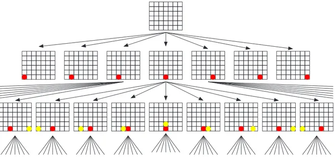
1.1 Portion of the state space for Connect-Four . . . 1
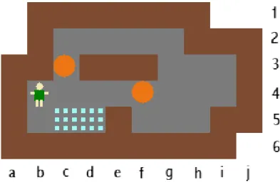
1.2 A Sokoban maze and a particular solution . . . 4
2.1 The finite search tree corresponding to an acyclic graph . . . 10
2.2 The infinite search tree corresponding to a cyclic graph . . . 11
2.3 The finite tree of all the possible acyclic paths of a cyclic graph . . . . 11
2.4 Invariant for depth-first search . . . 13
2.5 Invariant for depth-first search with cycle detection . . . 16
2.6 Invariant for breadth-first search . . . 23
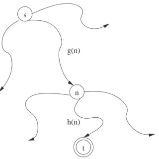
2.7 Construction of the heuristic estimate f (n) used by the A* algorithm. . 28
2.8 Invariant for the A* algorithm . . . 30
3.1 The last maze of our 90-problem benchmark . . . 44
3.2 Examples of deadlocks . . . 46
4.1 A Sokoban maze that is solvable stone-by-stone . . . 50
Introduction
Games have always fascinated mankind and attracted the attention of the AI research community. Writing game-playing programs is not just a diverting activity, it also has many applications in real-life problems. Indeed, when facing a problem humans often act as if they would be playing a game: they consider a number of different moves on their way to solve the problem. Some people consider even the life as a big game, where every alive being tries to maximize his well-being.
1.1
State-Space Representation
Classically, games are described as search problems. As an example, consider the game of Connect-Four. Given any game configuration, there is a finite number of moves that a player can make. Each of them leads to another position, which will allow the opponent a finite number of responses, and so on until it ends with a win or a tie. We can therefore represent the game of Connect-Four by considering each board situation as a node in a graph. The arcs in the graph represent legal moves from one board situation to another. These nodes correspond thus to different states of the game board. The resulting structure is called a state-space graph.
A path between two nodes of a graph is a sequence of arcs, such that the end point of any arc is the beginning point of the following one in the sequence. The problem of finding a particular path in a state-space graph is called a state-space problem. Figure 1.1 shows that starting the construction of the state-space graph with an empty board will lead to a graph representing all the possible games of Connect-Four.
1.1.1
Single-Player vs Multi-Player Games
Solving a single-player game requires to solve one state-space problem. Indeed, the game starts in a particular state and the program has just to find one path that leads to a goal node, i.e. a solution state of the game. The moves to play are then given by this path. This document mainly focuses on single-player games. As we will see, even if only one state-space problem needs to be solved, this will be far from trivial for interesting games.
In two-player games, the problem is not as easy, as finding one path that leads to a win does not really help. Indeed, this path will contain positions where it is the opponent’s turn. He will therefore have the freedom to decide what to play, not necessarily the moves of our winning path. In practice, two-player games are attacked with the minimax algorithm, but this is not covered in this document focused on single-player games 1. The problem becomes even harder when the number of opponents
grows.
1.1.2
Size of the Search Space
Obviously, the size of the search space plays a crucial role for solving state-space prob-lems. Intuitively, the depth of the solutions is also an important factor. The size of the search space of Connect-Four depicted in Figure 1.1, has been estimated at 1014 [1]. It
seems thus impossible to visit all states in reasonable time. We need more ingenious search strategies.
The problem of the size of the state-space graph is not specific to the game of Connect-Four. Indeed, all the interesting games are characterized by a huge search-space. A few more two-player examples are the game of Chess, where the state-space has been estimated at 10120, which is a number larger than the number of molecules in
the universe or the number of nanoseconds that have passed since the big bang [12], and the game of Go, where the size is even larger than for Chess, i.e. 10170 for the
classical 19 × 19 board [16]. A Single-Player example is the game of Sokoban, which will be the main focus of this document, and where the state-space is a cyclic graph estimated at 1098 [10].
1.1.3
Search Strategies
Many different algorithms have been created for exploring search spaces. They can be separated in two complementary groups:
• Blind methods, or uninformed search methods, do not use any problem-dependent information to guide through the search. They explore the state-space in a pre-defined way that is the same for all state-space problems.
• Heuristically informed methods use heuristics to determine in which order the different paths should be analyzed, i.e. to explore the most promising ones first.
A heuristic is a problem-dependent set of expert-rules for selecting lines that have a high probability of success. Heuristics are not foolproof: even the best game strategy can be defeated. For Connect-Four, the heuristic could for example be a function that favors paths leading to board configurations where the player’s tokens are strongly connected together and the opponent’s ones are dispersed all around the board.
The most popular strategy that uses heuristics is called the best-first search strategy. Humans use this natural strategy every day. For example, when planning to visit an old friend in another town, humans do not take the charts of all the existing roads of the world and explore all the possible combinations of roads until they found the best one leading to the desired destination. Instead, they use their experience to find a near-optimal route. When humans play games, they do not consider all possible moves in every possible position: they examine only moves that experience has shown to be effective. So heuristics can be seen as models of the experience of a problem.
Nevertheless, for some difficult games, machines are still far from beating humans and the research community mainly tries to do it with the existing modelling methods, focusing on new resolution methods. This document will instead introduce a new method, which seems to have never been tried till now. Actually, the main focus of this document will consist in proving that this method may lead to new interesting techniques and testing it on the game of Sokoban.
1.2
Multi-Agent Systems
According to [15], for game theorists a game is an abstraction of a situation where players, or agents, interact by making moves. Based on the moves made by the players, there is an outcome, or payoff, to the game. Standard games such as Poker and Chess are games in this sense. The game theorist’s notion of game, however, encompasses far more than what we commonly think of as games. Standard economic interactions such as trading and bargaining can also be viewed as games, where players make moves and receive payoffs.
1.3
The New Modelling Method
The heart of this thesis consists in exploring the idea that most single-player games can also be modelled as multi-agent systems. The agents are not, as usually, the players of the game, but more primitive game elements depending on the particular game. This leads to new interesting resolution techniques. This means thus that it will even be possible to solve single-player games using this multi-agent modelling approach.
1.3.1
The Game of Sokoban
The new game-modelling method will be demonstrated on a particular game: the game of Sokoban. This choice is not random. First, it is a one-player puzzle which has not been solved yet by the AI community. For now, the best documented solver called
Rolling Stone uses single-agent search techniques with a lot of problem-dependent
improvements, and is able to solve 59 problems of a difficult 90-problem test suite [10]. Furthermore, man still dominates machine in this domain.
Second, an unlimited set of different starting positions can be created by varying the size and the difficulty of the component problems. Different solving methods are therefore easy to compare, as there will always exist a test-set that can highlight the limits of the solving strategies. In this paper, we will compare our results to Rolling
Stone’s ones on the same 90-problem benchmark. The latter can be found at [6] with
their results. Chapter 3 will be dedicated to this game, explaining notably why it is so challenging. Let us just give the simple rules of the game yet, in order to be able to explain the contributions of this document in the domain.
A Sokoban maze is a grid composed of unmovable walls, free squares, exactly one man, and as many stones as goal squares. The player controls the man and the man can only push stones (not pull). Furthermore, only one stone can be pushed at a time. The objective of the game is to push all stones on goal squares.
Figure 1.2: A Sokoban maze and a particular solution: b4-c4-d4-e4-f4-g4-g3-g2-f2- e2-d2-c2-c3-c4-b4-b5-c5-c4-d4-e4-f4-g4-g3-h3-i3-i4-h4-g4-f4-e4-d4-e4-f4-g4-g3-g2-f2-e2-d2-c2-c3-c4. The corresponding stone-moves notation of the solution: f4-g4-h4, c3-c4-c5-d5, h4-g4-f4-e4-d4-c4-c5.
For a better understanding of the game, a solution to the problem of Figure 1.2 is given. It is first described as an ordered list of coordinates of the squares that the man must pass by, to bring all the stones on goal areas (starting with the initial square of the man). A shorter notation giving only the lists of the stone-moves is also provided. Note that this notation makes the implicit hypothesis that each stone-move of the solution is valid, i.e. that the man can reach the square adjacent to the stone to effectively make the push.
The idea of the new multi-agent representation is that every stone of the maze can be seen as an agent whose aim is to reach one of the goal squares, and the global goal is to find a solution for which everyone achieves his objective. It is also possible to impose some kind of optimality like minimizing the global number of agent moves. In this view of the problem, the man is only a puppet which can be called by the stones when they want to be pushed. It is important to note that the multi-agent notion which has been introduced is only conceptual and that it does not imply multi-agent programming. We will write an algorithm which requests a central solver to decide the order of the stones to be solved. This work presents thus solely a new way to view the problem which leads to new interesting resolution ideas.
We will define a particular subclass of Sokoban mazes that has been completely solved by a protocol based on our pure multi-agent representation. Intuitively, a maze is in this class if the stones are solvable one by one. Only one problem of our 90-problem benchmark is in the subclass (problem 78) and can be solved by this protocol. This is not surprising, as problems that are directly solvable stone by stone are uncommon in difficult benchmarks. Instead of elaborating other protocols for solving more general problems with the pure new multi-agent modelling approach, another idea has been developed.
As it is often the case in AI, trying to understand how the human player solves problems helps to find new algorithms. In the case of Sokoban, one of the talents of the human player consists in recognizing very soon in the resolution process that he can reach a configuration that is easy to solve (stone-by-stone). This suggests a new solving method for difficult games.
The method consists in using a classical state-space algorithm, but one in which the nodes whose corresponding state of the game is solvable by the new multi-agent modelling approach are defined as success nodes. This means that when the search reaches such a node, the search terminates successfully. The solution is then obtained by appending the solution path found by the state-space algorithm to the solution found by the multi-agent modelling method.
The offspring of success nodes are no longer reachable and can be considered to have been pruned out of the state-space. In practice, the size of the state-space will decrease substantially. On the other hand, more computation time is needed at each node as the multi-agent modelling approach is called for each node to determine whether it is a success node. However, the time lost by these calls is largely compensated by the time won by having less nodes to visit. Our program Talking Stones implements this idea.
At the time being, our program Talking Stones is not a contribution in the domain of Sokoban. It solves only 9 mazes of the benchmark whereas the state-of-the-art program
Rolling Stone solves 59. However, the latter is based on the IDA* algorithm with a lot
of really interesting problem-dependent enhancements. These are presented in [10] and it is well explained why each of them contribute to a substantial decrease of the search-tree size. On the other hand, the fact that no problem of the benchmark can be solved with the pure IDA* approach without these enhancements, even with a clever heuristic, is also demonstrated in [10]. We have not implemented these enhancements yet and we plan to inject them within our new method in future works. As Rolling stone has enjoyed tremendous progress by adding them to its initial pure IDA* approach (from 0 mazes solved to 59), we hope to benefit from the same kind of progression.
1.3.2
Classical State-Space Techniques
The classical state-space techniques can be reused in this approach, as tools that agents can use to solve subproblems of the game. For this purpose, the most popular best-first search algorithm will be intensively used: the A* algorithm [13, 14]. The latter will therefore be studied very carefully in this work. Note that even if the algorithm is presented in many AI books, it is often only presented at a rather high level and the fact that there exists a variety of possible practical implementations depending on the problem is often hidden 2.
This thesis will give an original presentation of the A* algorithm in particular and more generally of all the classical state-space algorithms. Usually, only a high-level description with abstract data types is given. Here we will present all the algorithms with the semi-formal-method proposed by [4]. The invariants specified in this work have not been taken from the literature. They have all been reconstructed from the original idea of the algorithm in order to produce a clear description of the latter and to prove its correctness. This approach has even led to a contribution for the A* algorithm. For one particular implementation choice for the abstract objects, we have discovered that it is possible to rewrite the algorithm in order to improve the practical performances.
1.3.3
Generalization of the Method
We can decompose the new solving method for difficult single-player games in three layers:
• The high-level layer is a classical state-space algorithm where a node is a success node if the medium layer can solve it. The choice of the algorithm depends on the characteristics of the game.
• The medium-level is a protocol based on a multi-agent representation of the game. The agents are primitive game elements depending on the particular game. The agents have to communicate together to find a common solution. They can use the algorithms of the low-level as tools for solving subproblems.
• The low-level is a set of algorithms for solving subproblems of the game. Classical state-space algorithms can be used but not exclusively.
We believe that it is possible for almost all games to determine primitive game elements that have to reach some goal. In puzzles like the 24-tile puzzle, the agents could be defined as the tiles. In this representation, each tile aims to reach its final destination but cannot move without altering the position of other agents. In the game of Sokoban, all the agents are instances of stones of the maze and have thus the same characteristics. For other games however, we could define agents that have their own personality. For the game of solitaire for example, the agents could be the 52 cards. Each agent is now unique. Note that for such imperfect information game, we must consider that only a subset of the agents is visible. The other agents can thus be seen as being in an unknown queue, waiting for entering into play.
2That does not mean that the well-known variations of the A* algorithm are often hidden. It
1.4
Overview of the Rest of the Document
Chapter 2 examines the most used search strategies. First, blind methods algorithms will be presented: the depth-first search and its variants, the breadth-first search and the iterative deepening depth-first search. Then, heuristically informed methods will be studied: the A* and the IDA* algorithm. Usually, only a high-level description with abstract data types of all these algorithms is given. Here we will present all the algorithms with the semi-formal-method proposed by [4]. The invariants specified in this work have not been taken from the literature. They have all been reconstructed from the original idea of the algorithm in order to produce a clear description of the latter and to prove its correctness.
Our new solving method will be demonstrated on the game of Sokoban. Chapter 3 introduces this game and give several arguments to show why this game is so chal-lenging. The precise definition of optimal Sokoban-solutions that we have chosen will than be given. We will justify briefly why we have chosen this definition instead of another also commonly chosen one. This chapter will also contain a short overview of the state-of-the-art in Sokoban programs.
Chapter 4 is dedicated to our new solving method applied to the real case of Sokoban. We will first define a particular subclass of Sokoban problem which have been completely solved by our multi-agent modelling approach. We will see that this class is too particular to be interesting for itself. However, we will see that it is possible to combine the iterative deepening algorithm that will be presented in chapter 2 with our new method and achieve better results. We will than give a generalization of the method and sketch how it could be used for other single-player games. Finally, different ways to extend the method will be suggested for future works.
Single-Agent Search
This chapter will describe classical search strategies commonly used for solving state-space problems. Deliberately, the most important strategies have been selected, letting other approaches in the dark. For more information, consult the references used in this chapter: [2, 7, 12, 17]. In this document, all the algorithms will be presented with the semi-formal method and the pseudo-code proposed by [3, 4].
2.1
Framework Presentation
2.1.1
The State-Space
Recall that a state-space problem consists in finding one path between a starting node and a goal node of a state-space graph. If the graph models a game, the states represent positions of the game board. The states are obviously problem-dependent. It must thus be supposed that the following data type is given:
type STATE = "problem-dependent";
The state-space graph is of course not present in memory. The space needed for stocking it would be too large for interesting problems. In fact, it is not necessary: each state-space algorithm starts with a beginning node and uses a function to generate the successors of the nodes that it wishes to expand. Typically, it is a function that "knows" the rules of the game and can compute all the possible moves in a given situation, obtaining the list of all the possible one-move modifications of the board. The following data type can thus be defined and the following function must be provided by the application:
type SUCCESSORS = list of STATE; 1
find-successors(s: STATE): SUCCESSORS;
⇒ function that returns the list of the successors of the state s.
1list can be implemented as a linked list. It would take us too far away from the purpose of this
document to explain in details how this can be done. We will restrict ourselves to specifying useful functions and procedures for manipulating lists. For a detailed implementation of linked lists, consult [3]. Note just that in this implementation, the constant nil is used to represent the empty list and that we will use the same convention here.
Our goal is to find a solution path, i.e. an ordered list of the states through which the game must evolve to reach a goal node. The different state-space algorithms will in fact manipulate lots of paths before finding the target one. This will be an essential data type of our framework:
type PATH = list of STATE;
Finding a goal node requires to know what a goal is. It depends of course of the problem studied. The following function must therefore be given:
goal-node?(s: STATE): boolean;
⇒ predicate true if and only if s is a goal state.
2.1.2
Useful Functions and Procedures
As lists will be intensively used by all search strategies, let us directly define useful functions and procedures that manipulate them, supposing that ELEM is the type of the elements of the list:
• initialize-list!(var l1: list of ELEM);
⇒ procedure that initialize the list l1 as an empty list.
• insert-front!(x: ELEM; var l1: list of ELEM);
⇒ procedure that inserts the element x in front of the list l1.
• insert-back!(x: ELEM; var l1: list of ELEM);
⇒ procedure that inserts the element x at the end of the list l1.
• get-first(l1: list of ELEM): ELEM;
⇒ function that returns a copy of the first element of the non-empty list l1.
• remove-first!(var l1: list of ELEM): ELEM;
⇒ function that removes the first element of the non-empty list l1 and returns
this element.
• append(l1, l2: list of ELEM): list of ELEM;
⇒ function that returns the concatenation of the lists l1 and l2.
• empty?(l1: list of ELEM): boolean;
⇒ predicate true if and only if l1 is the empty list.
• member?(x: ELEM; l1: list of ELEM): boolean;
⇒ predicate true if and only if x is an element of l1.
A constant for the empty list is also useful: const EMPTY_LIST = nil;
2.2
Graph Search is Really Tree Search
In this chapter, strategies for solving state-space problems in state-space trees will be given. In this section, the fact that graph search unfolds into tree search so that some nodes are possibly duplicated will be demonstrated.
As explained in the previous section, the graph is not present in memory. Each search strategy starts with the initial state of the problem and use the function
find-successors for generating the find-successors of previously generated nodes. The order
in which they are generated and removed from memory depends on the particular algorithm. To be more precise, nodes are generated for expanding previously generated paths until a path leading to a goal node is found (the first path being the one-node path which contains only the initial state of the problem).
Conceptually, the different search strategies can therefore be seen as various ways to explore the tree of all the possible paths that can be constructed from the initial state of the graph. This construction is only virtual and will never be computed. It is just useful for explaining the algorithms and proving their correctness. This section will be organized in two complementary parts: the cases of acyclic and of cyclic graphs.
2.2.1
Acyclic Graphs
A cycle is a path that contains at least two nodes that represent the same state of the problem and that are therefore labelled with the same etiquette (we will call such nodes
clones). Acyclic graphs are graphs that contains no cycle. The state-space graph of
the game of Connect-Four presented in chapter 1 (Figure 1.1) was an example of such a graph. Indeed, after each move the number of chips increases and the same position can therefore not occur twice in the course of the game (but can be reached in several ways, i.e. by several paths).
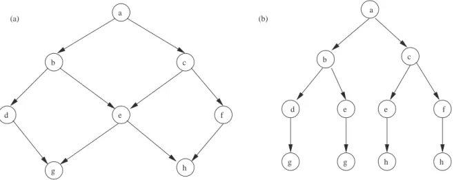
For an acyclic graph, the number of possible paths is finite and the tree representing all the possible paths of the graph is thus finite too. Figure 2.1 shows an example of the conceptual construction.
(b) b c d e f g h a a b c d e e f g g h h (a)
Figure 2.1: (a) An acyclic state-space graph: a is the start node. (b) The tree of all the possible paths from a.
2.2.2
Cyclic Graphs
Cyclic graphs contains at least one cycle. The state-space of Sokoban is an example of such a graph. Indeed, the man can push a stone to the left, come back to push it on its starting square, and finally come back on its own starting square, attaining the same state of the game again.
For a cyclic graph, the number of possible paths is infinite and the tree representing all the possible paths of the graph is thus infinite too. Figure 2.2 shows an example of the conceptual construction.
... b c d e g a (a) (b) a b c d e c a e g a e b b c d e c a e ... ... ... ... ... ... ... ... ...
Figure 2.2: (a) A cyclic state-space graph: a is the start node. (b) The infinite tree of all the possible paths from a.
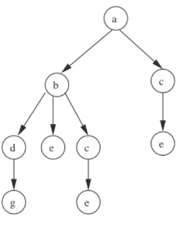
The good news however is that the nodes (and in particular the goal nodes) of the graph have all at least one clone at a finite level of the tree. This can be deduced by the fact that the graph has only a finite number of acyclic paths that starts at the root node. A finite tree of those acyclic paths can thus be constructed, as showed on Figure 2.3 for the graph of Figure 2.2.
e a
b c
d e c
g e
Each node of the graph appears exactly once in the tree, and the infinite tree containing also the cyclic paths is obviously only an extension of this tree. Algorithms that visit all the nodes at a particular depth before exploring deeper nodes will therefore terminate if a goal node exists. Algorithms with cycle detection (which avoid cycles) will only explore the tree of the acyclic paths and terminate thus even when no goal node exists. Some algorithms will however have no termination guarantee.
In the rest of the chapter, we will only consider the types of tree presented in this section. The trees can therefore be either finite or contain cyclic infinite branches. No trees with acyclic infinite branches will be considered (the only way to obtain such a tree would consist in starting with an infinite graph, but games are characterized by huge but finite graphs).
2.3
Blind Methods
This section presents algorithms for finding one path in a state-space tree, given no information about how to order the choices at the nodes.
2.3.1
Depth-First Search
The easiest way to explore the state-space tree consists in using a direct depth-first strategy. The idea of this search is simple. To find a goal node from a given node N, if
N is already a goal node the search terminates, else pick one of the children of N and
work forward from that node2. Other possibilities at the same level are memorized and
will be explored only when there is no more chance of reaching a goal node using the original choice.
The idea of the algorithm consists in working with a list open of paths to expand (a stack is appropriate too). Initially, it contains only one path: the path between the initial state of the problem and itself. At each iteration, the first path of open is extracted. If this path ends with a goal state, a solution path is found. Else, new paths are created by extending the removed path to all successors of the terminal state, and the new paths are added to the front of the list. The algorithm terminates when the solution path is found (it is then the first element of open), or when open is empty (no solution). However, we will see that for some kind of state-space trees the algorithm will never reach one of those termination cases.
For efficiency reasons, the paths will not be represented as usually as the ordered list of its constituting nodes from the starting to the final one. Indeed, testing if the final node is a goal node would require time proportional to the length of the list. Therefore, the paths will be represented in the reverse order: from the final node to the initial one of the sequence. This leads to a constant time, as the final node is yet the first of the list and can be accessed immediately.
2In this chapter, we will suppose that the successors are picked from left to right. Note that this
hypothesis is not constraining as the construction of the tree is only conceptual. The successors will be generated by the function find-successors and it can be decided where they will be placed in the virtual tree. Thus, this notion of left and right does only exist in the conceptual tree and not in the original problem.
2.3.1.1 Invariant
The invariant will be constructed using the following virtual coloring of the nodes:
• White nodes: nodes that have not yet been generated by the search.
• Blue nodes: nodes that have been generated but not visited. A node is said to be visited if we know that it is not a goal node.
• Green nodes: nodes that have been visited and that have at least one blue off-spring.
• Black nodes: nodes that have been visited and whose offsprings have all been visited.
The strategy of the depth-first search consists in keeping all the possible path from the root node to a blue node in open, and to order them in favor to the deepest and in case of a tie the leftmost blue nodes. At the beginning of the algorithm, all the nodes of the conceptual tree are white except the initial state of the problem which is blue. At each step of the algorithm, if the first node of the first path of open (the deepest blue node and in case of a tie the leftmost one) is a goal node the algorithm terminates. Else, it depends on whether this node is:
• An inner node: the node is colored green and its successors are all colored blue.
• A leaf: the node is colored black as well as all its ancestor that have no blue brother.
Figure 2.4 shows an example of the coloration after a few steps for a particular tree.
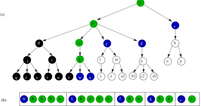
w b a b a b a b a a (b) w k e x k e f g c a b (a) e h l m n o p y z a2 b2 c2 d2 c d f g q r s t u v x k i j
Figure 2.4: Schematized view of the coloration before the path w-k-e-b-a will be ex-tracted from open: (a) The state-space tree. (b) The contents of open.
This coloration is only conceptual and will not be implemented. It is just useful for constructing a simple invariant that helps understanding the algorithm and proves its correctness. The strategy of the depth-first search can now be expressed as maintaining the following invariant:
P : open is composed of all the possible paths between the root node
of the tree and a blue node (ordered in favor to paths constructed from the deepest blue nodes, and in case of a tie the leftmost ones). The black nodes are all the left brothers of the green nodes and of the deepest and leftmost blue node. The white nodes are all the offsprings of the blue nodes.
The guardian B of the loop is true as long as open is not empty and as the first node of the first path of open is not a goal node. This means that after the loop testing if open is empty permits to decide whether a solution has been found or not.
2.3.1.2 Program
function depthfirst(start-state: STATE): PATH; var first-state: STATE;
first-path: PATH; open: list of PATH;
successor-list: SUCCESSORS; begin
initialize-list!(first-path); insert-front!(start-state, first-path); initialize-list!(open); insert-front!(first-path, open); {P}
do not empty?(open) cand not goal-node?(get-first(get-first(open))) → first-path := remove-first!(open);
first-state := get-first(first-path);
successor-list := find-successors(first-state);
"Add all the possible expansions of first-path with nodes of successor-list in front of open" {P}
od; {P and not B}
if empty?(open) → depthfirst := EMPTY_LIST ¤ not empty?(open) → depthfirst := get-first(open) fi
end.
The operation "Add all the possible expansions of first-path with nodes of
successor-list in front of open" can easily be computed. We can consider that the nodes of successor-list are ordered from right to left. This hypothesis can again be formulated
without restriction because the tree is conceptual and the location of the successors in the virtual tree can thus be chosen. From this, a simple loop solves the problem. At each iteration, the first successor is removed from successor-list, a new path is created by adding this successor in front of first-path and the created path is added in front of
The simple invariant of this inner loop can be stated as follows:
P2: successor-list contains consecutive successors of the first node of
first-path ordered from right to left and open begins with all the
possible one-node expansions of first-path created with successors that are not in successor-list and ordered from left to right.
In fact, before the loop, successor-list contains all the successors and open begins with no expansion of first-path. At each step, the first node of successor-list is removed and the corresponding expansion is added in front of open. The guardian B2 of this
inner loop is true until successor-list is empty.
{P2}
do not empty?(successor-list) →
insert-front!(insert-front!(remove-first!(successor-list),first-path),open) {P2}
od {P2 and not B2}
The final code is obtained by replacing in the main code the operation "Add all the
possible expansions of first-path with nodes of successor-list in front of open" by the
code of the inner loop here above.
2.3.1.3 Termination
The termination of the inner loop is trivial. The command remove-first!(successor-list) is executed at each iteration, so the size of successor-list will be decremented. The loop will thus end after a number of iteration equal to the size of successor-list. As the latter has been produced by the function find-successors and as this function returns a finite list of successors, the number of iteration will be finite too.
The main loop is more critical. Actually, we have no termination guarantee for general state-space trees. Indeed, if an infinite branch exists in the tree and if the first goal node is situated to the right of the first infinite branch, it will never be found. In fact, the nodes of the infinite branch must all be colored green before nodes situated to the right of the branch will be considered and it would take an infinite time to color them.
Intuitively however, if the state-space is finite this problem will not appear and the main loop will terminate. More formally, in a finite tree, the number of possible paths is finite. Therefore, the number of new paths that can be added to open is finite. At each iteration, a path is removed from open and new paths are potentially added. By construction, the same path cannot be added twice. This means that after a finite number of iteration, it will be impossible to add new paths to open. From this point, paths will only be removed and the size of open will decrease. The loop will terminate when the list is empty.
The efficiency of the depth-first search algorithm will only be investigated at the end of this section, where a comparison between the different blind methods will be done. The condition that the tree should be finite is worrying, as it will not be the case for many games. The program proposed in the next subsection solves this problem.
2.3.2
Depth-First Search with Cycle Detection
This algorithm is only a slight modification of the pure depth-first algorithm where only the finite sub-tree of the acyclic paths of the state-space tree is explored. A list
open will again be used but this time only acyclic paths will be added. To achieve this,
only the successors that have no clones in the current path will be used for expansion.
2.3.2.1 Invariant
The invariant will once again be constructed using a virtual coloring of the nodes. The definition of the different colors remains the same but the notion of visited has changed. A node is now said to be visited if we know that it is not a goal node or if we know that it is a clone of one of its ancestors.
To achieve the new coloration of the nodes, the same coloring as before is used except for the case of inner nodes. The list of all the successors of the inner node is again generated but this time all the successors that are clones of one of their ancestor are colored black as well as all their descendant 3. The latter are indeed all clones, as
the offsprings of a clone are also offsprings of the original node. The successors that have not been colored black are then colored blue. If all the successors where colored black, then the treatment that was performed on leaf nodes will be performed on this inner node (directly after the black coloration) and the coloring mechanism continues.
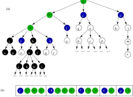
p p f f f e (b) b a k e b a f b a c a d a ... ... ... ... ... ... (a) a b c d j g a b c d h i q r b e f o p j k ... ... ... ... ... ... ... l b e m s k
Figure 2.5: Schematized view of the coloration before the path f-e-b-a will be extracted from open: (a) The infinite state-space tree. (b) The content of open.
3As a clone has an infinite number of descendant, an infinite number of nodes will have to be
colored black. However, recall that the coloring is only conceptual. That means that no infinite node-painting will be performed. The aim of this virtual coloration is only to model the fact that no acyclic solution exists in the subtrees of clones and that these nodes can be excluded from the search.
Figure 2.5 shows an example of the coloration after a few steps for a particular infinite tree. The invariant is only a slight modification of the invariant of the pure depth-first search algorithm:
P : open is composed of all the possible paths between the
root node of the tree and a blue node (ordered in favor to paths constructed from the deepest blue nodes, and in tie cases the leftmost ones). The black nodes are all the left brothers of the green nodes and of the deepest and leftmost blue node and all the children of the green nodes that are clones of one of their ancestor as well as the offsprings of those nodes. The white nodes are all the offsprings of the blue nodes.
2.3.2.2 Program
The main code is the same as before except that the operation "Add all the possible
expansions of path with nodes of successor-list that are not member of first-path in front of open" will be used instead of the other one.
This operation can be computed using a similar inner loop as before, with the difference that at each iteration, the new path with the first successor of successor-list is only created and added in front of open if this successor is not a member of first-path. The invariant P2 is the same as before except that we add "all the possible one-node
expansions of first-path created with successors that are neither in successor-list nor in first-path" instead of simply "not in successor-list". The guardian B2 is exactly
the same as before.
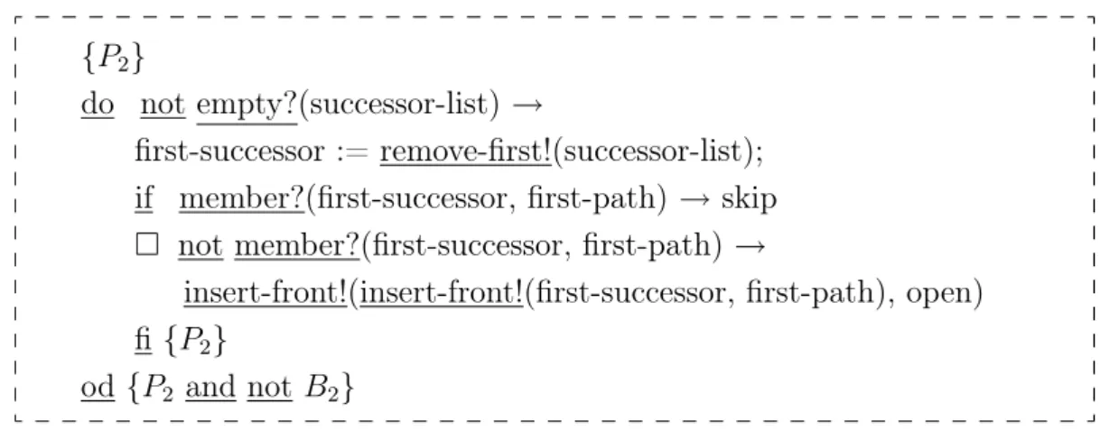
{P2}
do not empty?(successor-list) →
first-successor := remove-first!(successor-list); if member?(first-successor, first-path) → skip ¤ not member?(first-successor, first-path) →
insert-front!(insert-front!(first-successor, first-path), open) fi {P2}
od {P2 and not B2}
2.3.2.3 Termination
The termination of the inner loop can be proved with the same argument as before because the function remove-first! is once again called at each iteration. This time only acyclic paths are added to the list open. As we consider only infinite trees with cyclic infinite branches, the number of acyclic paths is finite and the same argumentation as before proves the termination of the main loop.
2.3.2.4 Variant
Another way to achieve this algorithm consists in keeping in addition to the open list of paths to expand, a closed list of the visited nodes. Instead of checking if a successor is in the path from which it was generated, the closed list will be consulted. The clones of already visited nodes will thus be detected directly.
The definition of the different colors remains the same but the notion of visited changes again. A node is now said to be visited if we know that it is not a goal node or if we know that it is a clone of a previously visited node. To achieve the new coloration of the nodes, the same coloring as usually is used except for the case of inner nodes. The list of all the successors of the inner node is again generated but this time all the successors that are clones of a green or a black node are colored black as well as all their descendant. The invariant P is easy to modify: the black nodes are all the left brothers of the green nodes and of the deepest and leftmost blue node and all the children of the green nodes that are clones of a green or a black node as well as the offsprings of those nodes. The invariant P2 must merely be adapted for
performing the membership test on closed.
function depthfirst-cycledetection(startstate: STATE): PATH; var first-state, first-successor: STATE;
first-path: PATH; open: list of PATH; closed: list of STATE;
successor-list: SUCCESSORS; begin
initialize-list!(first-path); insert-front!(startstate, first-path);
initialize-list!(open); insert-front!(first-path, open); initialize-list!(closed); {P} do not empty?(open) cand not goal-node?(get-first(get-first(open))) →
insert-front!(first-state, closed); first-path := remove-first!(open); first-state := get-first(first-path); successor-list := find-successors(first-state); {P2} do not empty?(successor-list) → first-successor := remove-first!(successor-list); if member?(first-successor, closed) → skip ¤ not member?(first-successor, closed) →
insert-front!(insert-front!(first-successor,first-path),open) fi {P2}
od {P and P2 and not B2}
od; {P and not B}
if empty?(open) → depthfirst-cycledetection := EMPTY_LIST ¤ not empty?(open) → depthfirst-cycledetection := get-first(open) fi
The termination of the inner and main loops are the same as for the first variant. The membership test will take time proportional to the length of closed. As closed contains also the states of the current path, this methods performs less efficiently than the preceding one. However, the advantage of this method is that for some problems,
closed can be implemented as an indexed vector or a hash-table instead of a list and
that the membership test will thus take a constant time. The first variant of the algorithm took time proportional to the length of the paths of open which are already implemented as list and it was therefore not possible to go faster.
2.3.3
Depth-Limited Depth-First Search
Another way to ensure to termination of the depth-first search algorithm is to limit the depth of the search. All the nodes situated deeper than the limit will be ignored and the algorithm terminates for all type of trees (even infinite trees with acyclic infinite branches). The problem of this method is that the goal nodes situated deeper than the limit are also neglected. The algorithm could thus conclude wrongly that no solution exists. It can therefore be used only when the fact that the first solution cannot be deeper than a certain depth is known a priori.
A simple but inefficient way to implement this search strategy would consist in modifying the classical depth-first algorithm such that paths of the same length as the depth limit are not expanded. The inefficiency comes from the fact that computing the length of a path takes a time proportional to its length. The classical implemen-tation consists therefore in memorizing the length of each path of open in another list called open-elem-sizes (keeping them both in the same list is of course also possible). Computing the length of a new created path consists now merely in adding one to the length of the path that was just expanded.
2.3.3.1 Invariant
The invariant will be constructed with the same coloring of the nodes as for the general depth-first search algorithm, except that we consider that the nodes that are deeper than the depth limit have all been colored black before the algorithm starts. As usually, this coloration is conceptual; in this case its only purpose is to model the fact that those nodes are ignored from the very start. The different steps of the coloring of the nodes remain the same as for the general depth-first algorithm except that when the successors of an inner node are black the inner node is considered as a leaf node. The invariant can now be defined as follows:
P : open is composed of all the possible paths between the root node
of the tree and a blue node (ordered in favor to paths constructed from the deepest blue nodes, and in tie cases the leftmost ones).
Open-elem-sizes is the list of the length of the path of open in
the same order. The black nodes are all the left brothers of the green nodes and of the deepest and leftmost blue node. The white nodes are all the offsprings of the blue nodes.
2.3.3.2 Program
function limited-depthfirst(start-state: STATE; depth-limit: integer): PATH; var first-state: STATE;
first-path: PATH; open: list of PATH;
open-elem-sizes: list of integer; current-size: integer;
successor-list: SUCCESSORS; begin
initialize-list!(first-path); insert-front!(start-state, first-path); initialize-list!(open); insert-front!(first-path, open);
initialize-list!(open-elem-sizes); insert-front!(1, open-elem-sizes); {P} do not empty?(open) cand not goal-node?(get-first(get-first(open))) →
first-path := remove-first!(open);
current-size := remove-first!(open-elem-sizes); if current-size = depth-limit → skip
¤ current-size < depth-limit → first-state := get-first(first-path);
successor-list := find-successors(first-state);
"Add all the possible expansions of first-path with nodes of
successor-list in front of open and actualize open-elem-sizes"
fi {P}
od; {P and not B}
if empty?(open) → limited-depthfirst := EMPTY_LIST ¤ not empty?(open) → limited-depthfirst := get-first(open) fi
end.
The operation "Add all the possible expansions of first-path with nodes of
successor-list in front of open and actualize open-elem-sizes" is a slight modification of the
corresponding operation of the depth-first search. The invariant P2 remains the same
except that a sentence must be added to express that open-elem-sizes must always contain the list of the length of the paths of open in the same order.
{P2}
do not empty?(successor-list) →
insert-front!(insert-front!(remove-first!(successor-list),first-path),open); insert-front!(1 + current-size, open-elem-sizes) {P2}
2.3.3.3 Termination
The termination of the inner loop is exactly the same as its counterparts. The termina-tion of the main program consists again in proving that the number of different paths that can be added to open is finite and that we will eventually reach a point where paths can only be removed. This is clear since the depth of the search has been limited and the explored tree is therefore finite and contains a finite number of different paths from the root.
The difficulty when using this algorithm is to chose a good depth-limit. A too small value would lead to a high probability that all the goal nodes are ignored and a too large value would lead to an important time complexity (non-solution paths will be expanded very deep wasting a lot of time). The next algorithm solves this problem.
2.3.4
Iterative Deepening
To avoid the difficulty of the choice of the depth limit, we can execute the depth-limited depth-first search iteratively by increasing the depth limit at each iteration until a solution is found. An integer current-limit will represent the current depth-limit. It will be initialized to zero and increased by one at each iteration. The variable
current-solution will be the returned value of the function limited-depthfirst for the
current depth-limit. Initially it will be the empty list and it will change only in the last iteration, i.e. when it becomes the least deep and leftmost solution path. The algorithm can then terminate and the guardian B which is true as long as current-solution is the empty list is appropriate. The algorithm makes obviously the hypotheses that at least one goal node exists. This is not worrying for practical games which have at least one finite solution.
2.3.4.1 Invariant
P : current-solution is the leftmost solution path of the state-space
tree that has a length exactly equal to current-limit (empty list if no such solution exists).
2.3.4.2 Program
function iterative-deepening(start-state: STATE): PATH; var current-limit: integer;
current-solution: PATH; begin
current-limit := 0; current-solution := EMPTY_LIST; {P} do empty? current-solution →
current-limit := current-limit + 1;
current-solution := limited-depthfirst(start-state, current-limit) {P} od; {P and not B}
iterative-deepening := current-solution end.
2.3.4.3 Termination
The algorithm terminates only if a goal node exists in the state-space tree. Recall that we consider only finite trees or infinite trees with cyclic infinite branches and that therefore at least one goal node must be situated at a finite depth if a goal node exists in the tree.
The advantage of this method is that it finds the shortest solution path. The algorithms seen till now did not have this convenient property. They find the leftmost solution paths and this is not necessarily the shortest. The inconvenient of the iterative deepening algorithm is that at each iteration, the paths previously computed have to be recomputed again. However, in the efficiency analysis of the different blind methods we will show that it will not affect the time complexity so much. Typically, when the branching factor is not too small, most of the time will be spent in the last iteration and repeated computations with lower limit values adds relatively little to the total time.
2.3.5
Breadth-First Search
This algorithm starts with the same idea as the depth-first search algorithm: to find a goal node from a given node N, if N is already a goal node the search is terminated, else another node of the state-space is picked and the algorithm works forward from that node. The difference is that the picked node is no more the leftmost child of the node, but the closest node to the start node that was not visited yet. When several such nodes exist, the leftmost one is conventionally chosen. Thus, if the previous picked node is not the rightmost of a particular level, the next picked node will be its right neighbour. Else, it will be the leftmost node of the next level. The algorithm progress thus in breadth, level by level. Hence the name of the algorithm.
The idea of the implementation consists in working with a list open similar to the one used by the depth-first search strategy. The only difference, is that all the expanded paths will be added to the back of the list instead of the front 4.
2.3.5.1 Invariant
The invariant will be constructed using the following virtual coloring of the nodes:
• White nodes: nodes that have not yet been generated by the search.
• Green nodes: nodes that have been visited. From now and for the rest of the document, the original notion of visited will be used (nodes that are known non-goal nodes).
• Blue nodes: nodes that have been generated but not visited.
4Note that in the implementation of lists as linked lists that we have suggested, it is possible to
keep two pointers that indicates the locations of the first and the last element of the list. The function
insert-back! can thus be implemented in time constant. The only operation that needs to be done is
merely to link the last element of the list (that was linked to nil) to the new element and to link this new element to nil.
At the beginning of the algorithm, all the nodes of the conceptual tree are white except the initial state of the problem which is blue. At each step of the algorithm, if the least deep and leftmost blue node is a goal node the algorithm terminates. Else, this node is colored green. If no blue node exists, all the nodes have been visited and no solution exists. As usual, this coloration is only conceptual and will not be implemented.
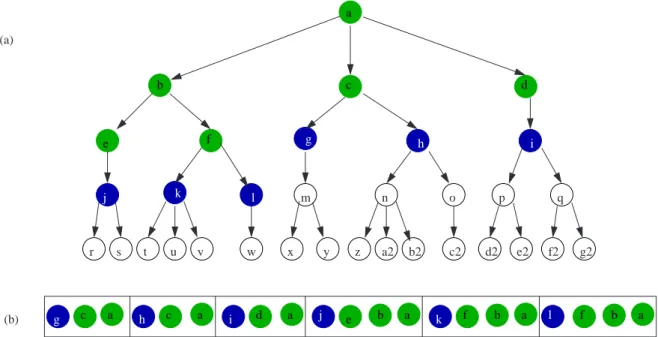
The strategy of the algorithm can be expressed as maintaining the invariant:
P : open is composed of all the possible paths between the root node
of the tree and a blue node (ordered in favor to paths constructed from the least deep blue nodes, and in tie cases the leftmost ones). The green nodes are the ancestor of the blue nodes and the white nodes their offsprings.
Figure 2.6 shows an example of the coloration and the corresponding contents of
open after a few steps for a particular tree.
a b c d e f c a c a d a e b a f b a f b a (a) m n o p q r s t u v w x y z a2 b2 c2 d2 e2 f2 g2 (b) j k l g h i g h i j k l
Figure 2.6: Schematized view of the coloration before the path g-c-a will be extracted from open: (a) The state-space tree. (b) The contents of open.
The main code is the same as for the depth-first search except that the operation
"Add all the possible expansions of first-path with nodes of successor-list to the back of open" is used instead of the other. This can be computed by considering this time
that the nodes of successor-list are ordered from left to right. Considering the opposite choice as for the depth-first case is not problematic. The explored tree is still conceptual and the nodes must not be placed at the same positions than for the depth-first search. A simple loop performs the operation. At each iteration, the first successor is removed from successor-list, a new path is created by adding this successor in front of first-path and the created path is added to the back of open. The paths added at the end of open will therefore be ordered in favor to the ones containing the leftmost successors and the invariant is preserved. The loop terminates when the list is empty. The simple invariant of this inner loop can be stated as follows:
P2: successor-list contains consecutive successors of the first node of
first-path ordered from left to right and open ends with all the
possible one-node expansions of first-path created with successors that are not in successor-list and ordered from left to right.
The guardian B2 is the usual one for the actualization of open, i.e. it is true as long
as successor-list is not empty.
{P2}
do not empty?(successor-list) →
insert-back!(insert-front!(remove-first!(successor-list),first-path),open) {P2}
od {P2 and not B2}
2.3.5.2 Termination
The termination of the inner loop can be proved with the usual argument. In fact, the function remove-first! is once again called at each iteration and successor-list will eventually become an empty list after a finite number of steps.
The algorithms terminates if a goal node exists at a finite depth. Indeed, at each iteration a node is colored green. Furthermore, no node is colored green before all the nodes of the less deep levels are all colored green. As the number of nodes of each level is finite, the level of the goal node will be reached after a finite number of steps and finding the goal in this level will also require a finite number of steps.
If no goal node exists, the algorithm terminates if and only if the state-space tree is finite. The fact that exactly one node is colored green at each iteration demonstrates this fact. Indeed, if the tree is finite, all the nodes will be green after a finite number of steps and the algorithm concludes that no solution exists. In the infinite case it would take an infinite time to color all the nodes and the procedure would never terminate.
2.3.5.3 Variants
A variant with cycle detection can also be constructed. Limiting the depth of the search makes however less sense as the algorithm works already level by level.
2.3.6
Efficiency Analysis
This subsection compares the main blind methods on two important measures of com-plexity:
• The time complexity: correspond to the order of magnitude of time needed for finding a solution. It is measured as the total amount of nodes generated by the search strategy until a solution is found.
• The space complexity: correspond to the order of magnitude of memory used during the execution of the algorithm. It is measured as the maximum number of nodes that must be kept in memory during the execution of the algorithm.
The different uninformed search methods will be compared on a generic state-space tree for which each inner node has exactly b successors and the only solution is the rightmost node situated at a depth d. This is the worst place possible at depth d because we have supposed that the different strategies works from left to right. Note that the performances of all algorithms become better when the first solution moves to the left, but this can only occur by chance as an uninformed method cannot order the nodes so that the most promising are explored first.
The number of nodes grows exponentially with the depth, so the number of nodes generated by the breadth-first search strategy is 1+b+b2+b3+.... The time complexity
is thus O(bd). The breadth-first search maintains all the bdcandidate paths in memory.
Those paths are composed of a maximum of d nodes and the space-complexity is thus
O(bd) too.
In the depth-first search category, we will not consider the pure algorithm because it has no termination insurance and both complexities may be infinite. We will rather study the complexities of the depth-first search limited to a depth of dmax so that d ≤
dmax. The total number of nodes of the depth-limited tree is bdmax and the nodes will all
be generated except the offspring of the solution node. The time complexity is therefore
O(bdmax). With a cycle-detection mechanism, the complexity remains generally the same except for special state-space trees for which the number of cycle is very high.
The maximum number of nodes in memory occurs when the search has reached the leftmost leaf. At this precise moment, the number of green nodes is dmax − 1;
i.e. all the nodes of the leftmost branch except the leaf. The number of blue nodes is (b − 1) × (dmax− 1) + 1; i.e. each green node has exactly (b − 1) blue children except
the deepest one which has one more. The number of paths in memory is equal to the number of blue nodes. All paths are bounded by a size of dmax. The space complexity
is therefore only O(d2 max).
The iterative deepening algorithms performs (d + 1) depth-first searches limited respectively by a depth of 0, 1, ..., d. The maximum number of nodes in memory oc-curs in the last iteration when the search reaches the leftmost node of depth d. The same argumentation as for the depth-limited depth-first search shows that the space complexity is O(d2).
The start node will be visited (d + 1) times (at each iteration), the children of the start nodes d times (at each iteration except the first one), etc. The number of generated nodes is thus:
(d + 1) × 1 + d × b + (d − 1) × b2 + ... + 1 × bd
This gives also a time complexity of O(bd). The conclusion is that even if the
iterative deepening seems very coarse at the first glance, the regenerating of nodes is in fact surprisingly small. It can be shown that the ratio between the number of nodes generated by iterative deepening and those generated by breadth-first search is approximately b
b−1 for b ≥ 2 [2]. This means that when the branching factor is high
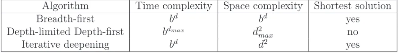
the difference becomes practically unnoticeable. The following tabular summarizes the conclusions:
Algorithm Time complexity Space complexity Shortest solution
Breadth-first bd bd yes
Depth-limited Depth-first bdmax d2
max no
Iterative deepening bd d2 yes
Table 2.1: Efficiency comparison of the three main blind methods
The column Shortest solution indicates whether each algorithm finds the shortest solution first or not. For some problems however the arcs may have different costs and the optimal solution would not be the shortest but the one for which the sum of the costs of the arcs is minimal. It is not possible to achieve such optimality with the pure blind methods presented here. The A* and IDA* algorithms presented in the next section are designed to ensure this cost-optimality.
The cost of an arc is a number which indicates how difficult it is to make the problem evolve from the initial state of the arc to its target state. For some problems it is indeed convenient to do so. Consider for example a path-finding application. A robot must go from its starting point to a target point of a game area. The latter is composed of forest, lakes and deserts. We could for example consider that it is more difficult to travel through a forest than a desert, and even more difficult to traverse a lake. A convenient way to model this is to associate a cost of 1 to the arcs that represents a one-step move in the deserts, 2 in the forest and 3 in a lake. The problem is now to find the solution-path with minimum cost.
The iterative algorithm combines obviously the best properties of breadth-first search and depth-first search. It is thus often the best choice for practical AI problems when the problem is not too complex. The depth-first search algorithm is also very of-ten used. The language PROLOG for example works in depth-first manner. However, the blind methods that we have seen make nothing to fight against the combinatorial explosion because they consider each possibility to be equally probable. For complex AI problems, methods based on heuristics are more appropriate. This is the subject of the next section.
2.4
Heuristically informed methods
In chapter 1 we have seen that a heuristic is a function for selecting lines that have a high probability of success. The search efficiency may improve spectacularly by using clever heuristics to guide through the search. In this section, the most famous algorithm that uses heuristics and its most important variant will be presented: the A* and IDA* algorithms.
From now, we will suppose that a cost has been associated to the arcs of the state-space tree. This means that a function cost(s1, s2) defines the cost of moving from
each state s1 of the state-space tree to each successor s2 of s1. If the problem does not
require to associate different costs to the arcs, the function will simply use a value of 1 for each.