HAL Id: dumas-00802143
https://dumas.ccsd.cnrs.fr/dumas-00802143
Submitted on 19 Mar 2013
HAL is a multi-disciplinary open access
archive for the deposit and dissemination of sci-entific research documents, whether they are pub-lished or not. The documents may come from teaching and research institutions in France or abroad, or from public or private research centers.
L’archive ouverte pluridisciplinaire HAL, est destinée au dépôt et à la diffusion de documents scientifiques de niveau recherche, publiés ou non, émanant des établissements d’enseignement et de recherche français ou étrangers, des laboratoires publics ou privés.
The economic geography of Europe and the role of
regional policy
Julian Hinz
To cite this version:
Julian Hinz. The economic geography of Europe and the role of regional policy. Economics and Finance. 2012. �dumas-00802143�
The Economic Geography of Europe
and the Role of Regional Policy
∗Julian Hinz† June 2012
Supervisor: Matthieu Crozet Second Reader: Lionel Fontagn´e
Abstract
In this thesis I set up a standard New Economic Geography model and estimate it in the regional context of the European Union. The analysis underlines the clear core-periphery structure of Europe, but also identifies forces that hint at a catching-up of lesser developed peripheral regions. While regions that are close to the geographic center on average have a much higher market access, regions far from the center can improve their market access over the time period of 1999 - 2009 relative to their initial position. I estimate and evaluate the impact of European Union Cohesion Policy on this process and do not find the positive developments to be caused by or connected to the financial facilities of the European Union Regional Policy.
∗I thank Matthieu Crozet for supervising this Master thesis and for his help. I am grateful to Sandy Dall’erba and Julie le Gallo for their help sharing and commenting on data on European Regional Policy. I thank Holger Breinlich for further comments on his research. I am thankful for the invaluable help of Rose von Richthofen and Nilofar Saidi.
1
Introduction
“The Community shall have as its task [...] to promote throughout the Community a harmonious, balanced and sustainable development of eco-nomic activities [...], the raising of the standard of living and quality of life, and economic and social cohesion and solidarity among Member States.” — Article 2 of the Treaty establishing the European Community (1957)
The European Union has had a profound impact on the Economic Geography of the European Continent. The creation of the community in 1958 with the Treaty of Rome (1957) marked the starting point of an ever closer political and economic integration of a growing number of countries. In 2012, with now 27 member states, the political entity has more than half a billion inhabitants speaking in 23 official languages, that account for approximately 20% of the world’s GDP (European Commission, 2008a). Although the community has evolved into a highly integrated union, economic and social disparities have remained high. 43% of the European Union’s economic output is generated in just 14% of its territory (European Commission, 2008c), particularly in the core situated in the geographic center of Europe. The peripheral regions are characterized by on average higher unemployment rates and a lower GDP per capita, emphasizing the strong core-periphery structure.
The economic integration of Europe has been at the heart of the entire integration process. The removal of borders and the introduction of one market for goods, the possibility for citizens of the EU to roam, live and work freely in any member country are known to have a vast impact on the economic geography of the continent (Crozet & Lafourcade, 2009, p. 79). The introduction of a single currency in wide parts of the political union, further reducing barriers for the internal market, has surely contributed to this end. In the context of the monetary integration and in light of Mundell (1961)’s criteria for an optimal currency area, Dall’erba (2008) recognizes that when “countries loos[e] control over monetary policy, cohesion policies [are] sometimes seen as the only tool to cushion asymmetric shocks and structural problems.”
Since the Treaty of Rome in 1957, the European Community and later the European Union has the task “to promote throughout the Community a harmonious development of economic activities, a continuous and balanced expansion, an increase in stability, an accelerated raising of the standard of living and closer relations between the States belonging to it” (Treaty of Rome, 1957, Article 2). With establishing the Structural
Funds and later the Cohesion Fund, this task received financial firepower.
EU regional policy has the aim to promote cohesion in economic, social and territorial terms for regions in the European Union. The size of the allocated funds is regularly about a third of the entire EU budget (European Commission, 2008b). The funds
are allotted via different mechanisms to account for different objectives. In the pe-riod of 2000 - 2006 the two most important among others were defined as (European Communities, 2004):
Objective 1, for which roughly 80 percent of funds were transferred to regions, was the
aim in NUTS2 regions where the GDP per capita is less than 75 percent of the EU25 average. Almost all regions of the new member states were covered by this objective. The primary obstacles to prosperity in these regions were assumed to be a general low level of investment, high unemployment and the lack of basic infrastructure.
Objective 2, for which about 16 percent of the available funds were allotted to, was
the aim in the regions that were facing a structural change in previous key sectors, most notably declines in industrial activity and other traditional activities, leading to unemployment.
The Cohesion Fund provided another source of infrastructure funding and co-financing for countries that had a GDP of less than 90% of the EU average, covering similar areas as Objective 1.
In prior programming periods from 1989 - 1993, 1994 -1999 the aims were named dif-ferently and varied in numbers, the general objectives were of course closely related to the current ones. In the current period of 2007 - 2013, Objective 1 has been re-named the convergence objective and Objective 2 is part of the competitiveness and
employment objective (European Commission, 2008a). The allocated funds are aimed
at promoting economic growth and improved competitiveness on a regional level. This is to be achieved via several channels, most notably in infrastructure, human capital formation and social inclusion.
These policies have naturally been subject to economic research. Most of the econo-metric evaluations of European Union Regional Policy and its economic impact are situated in the Economic Growth literature, employing very different techniques lead-ing to no coherent picture of the results (Dall’erba & Le Gallo, 2008). Among the notable contributions are Rodriguez-Pose & Fratesi (2004), employing a cross-sectional panel data analysis finding spending on infrastructure through Objective 1 funds to have an insignificant effect and only investments in human capital and education to have a medium run significant positive return. Becker et al. (2010) exploit the afore-mentioned threshold of a GDP below 75% of the average GDP for the eligibility for Objective 1 regions to identify causal effects of the receipt of funds on economic growth in the respective regions. Other authors, such as Dall’erba & Le Gallo (2008) and Gallo
et al. (2011) employ spatial econometric techniques to account for spatial linkages in
The main strand in economic research that is concerned with spatial features is of course Economic Geography, analyzing the roots and effects of agglomeration economies. The core-periphery concept, of apparent interest when studying the case of Europe, has received wide attention at least since the seminal contribution of Krugman (1991), a turning point for the henceforth New Economic Geography, emphasizing the inter-play between proximity to markets for demand and supply, prices for input factors and trade costs.
The notion of market access has created a burgeoning literature with a wide range of topics. Hanson (1998, 2005) and Redding & Venables (2004) were successful in porting the theoretical advances to empirical tests. Redding & Venables (2004)’s econometric approach has been particularly influential, deriving a structural equation that relates wages to the proximity to demand and supplier markets, and achieving to explain a large part in the international variation of income with geographic features. Head & Mayer (2011) extend this analysis over a long period of time to find a long-term impact of market access on the economic development of countries.
Hanson (1998, 2005)’s work focusses on the subnational level, estimating the effects of market access on wage differentials for US counties. Other research applying this theoretical framework to country-level data include Brakman et al. (2004), who study the case of Germany.
A different strand of the economic geography literature exploits historical coincidences as a form of natural experiments: Redding & Sturm (2008) use the German partition and reunification between the end of World War 2 and 1990 showing the importance of market access through a decline of population in border areas, as suggested by the theory. Davis & Weinstein (2002) test the durability of economic geography against external shocks, analyzing the population distributions before and after allied bomb-ings of World War 2 on Japanese cities, finding a strong persistence of established economic geographical patterns.
In the European context, a number of works stand out. Head & Mayer (2004) use a similar framework as Redding & Venables (2004) to develop a model of location choice for firms, and show using data on Japanese investments in Europe that investments are made “where the markets are”, focussing the research on the backward linkages to demand sources. Crozet (2004) sheds light on the forward linkages, developing and estimating a model of individual location choice with interregional migration data for five European countries. Combes & Overman (2004) provide a survey over literature and open questions over for the specific case of Europe.
Breinlich (2006) follows closely the methodology and focus of research of Redding & Venables (2004) and applies the framework to European regions, identifying human capital accumulation as a channel through which market access influences wages. Head & Mayer (2006), also focussing on European regions, modify the approach slightly and
are looking at wage and employment responses to proximity to markets for different industries.
This paper also makes use of the Redding & Venables (2004) methodology and through its European focus is closely related to Breinlich (2006) and Head & Mayer (2006). It extends the analysis to all 248 regions of the 25 member states of 2006 that were located in continental Europe. Analyzing the determinants for the economic geography of Europe, I estimate the impact of Objective 1 (and Cohesion Fund) and Objective 2 facilities on the dynamics and determinants of the distribution of income.
The paper is organized as follows: In section 2 I set up the theoretical framework in which I am to analyze the Economic Geography of Europe. The following sections are concerned with the empirical testing of this model, where the trade equation is estimated and market access is calculated (Section 3) and these results then used in the estimation of the wage equation (Section 4). In section 5 I draw the link to the policy dimension and estimate the role of European Union Regional Policy in the determinants for change of the distribution of income across Europe. Section 6 finally concludes.
2
Theoretical Framework
In this section I set up a standard New Economic Geography model, modified for the purpose of an analysis of regional wage differences. The framework is fundamen-tally based on Fujita et al. (1999), and comparable to Redding & Venables (2004), while highlighting the regional approach similar to Head & Mayer (2006) and Breinlich (2006). I loosely follow the notation of Combes et al. (2008) for its ease of use and readability.
The model is made up by R regions, where in each region r there are nr firms that
produce their variety of a good qr. The consumer in region r, who derives his income Yr from wages wr and rent on capital xr, and spends a fraction µr on the produced
products from region r and all other regions s∈ R. In the following, r is to be perceived as the domestic region, whereas s is a foreign region, simplifying the understanding of the model.
2.1 Supply Side
As usual, the model consists of a supply and demand side. On the supply side, for the firm in region r to produce one unit of its product, it is faced with a function
qr= ALαrXrβ − a (1)
with α + β = 1
where in the Cobb-Douglas function-like component Lr is the labor input, α the
as-sociated labor share in income, Xr the input of capital and β the share of capital in
income. A is a standard technological parameter and a is a fixed input which deter-mines the degree of increasing returns to scale, both are assumed to be identical across all regions.
The firm maximizes the production of its variety qr while operating under a cost
constraint. The optimization problem is therefore: max
Lr,Xrqr
= ALαrXrβ− a
s.t. Cr= wrLr+ xrXr
The optimization leads to the cost function
Cr = wαrxβr (qr+ a)
For the firm this implies a profit
Πr= R
∑
s=1
prqrs− wαrxβr (qr+ a)
This introduces the notion of distance, as qrs is the quantity of a variety qr that is
produced in region r and then sold in (or exported to) region s. Splitting the cost into fixed and marginal cost this becomes
Πr= R
∑
s=1
prqrs− mrqr− Fr (2)
with the marginal cost mr= wαrxβr (3)
and the fixed cost Fr= awαrxβr (4)
The operating profit of a firm in region r exporting to region s in equilibrium is then
with an equilibrium mill price p∗r, the equilibrium quantity qrs∗ and trade cost τrs ≥ 1.
The trade costs are ad valorem, or so-called iceberg trade costs, meaning a fraction of
τrs−1
τrs of the shipped goods “melts” on the way from region r to s. Under increasing returns to scale and imperfect competition, the firm establishes an equilibrium price for the consumer1 of
p∗rs= τrsp∗r= τrsmr ( σ σ− 1 ) (6)
receiving a markup of σ−1σ over the marginal cost. Substituting (6) into (5) yields
π∗rs= mr τrsqrs∗
σ− 1 (7)
2.2 Demand side
On the consumer side, the equilibrium demand qrs∗ for goods in region s from region r is derived from the consumer’s utility maximization. The agent is assumed to have a preference for consuming all available varieties from all regions R, characterized by a CES utility function:
max qrs Us= ( R ∑ r=1 nrq σ−1 σ rs ) σ σ−1 (8) s.t. R ∑ r=1 nrprsqrs = µsYs
As described above, Ysis the income in region s, µs the share of income devoted to the
consumption of the considered good, σ the elasticity of substitution, nr the number of
varieties in region r. The optimization leads to
qrs∗ = p−σrs ∑RµsYs
r=1nrp 1−σ rs
(9)
which can be further simplified by defining a price index Ps
q∗rs= p∗−σrs µsYsPsσ−1 (10) with Ps = ( R ∑ r=1 nrp∗1−σrs ) 1 1−σ (11)
The equilibrium quantity exported from region r to s is therefore negatively dependent on its price, and positively dependent on the share of income devoted to consumption of this good, discounted by the price level in the importing region.
1
Multiplying (10) on both sides with nrprs yields
nrp∗rsq∗rs= nrp∗1−σrs µsYsPsσ−1 (12) which I will call the trade equation in accordance with previously mentioned authors using a similar setup and following Redding & Venables (2004). This equation will be estimated in section 3.1.
Returning to the firms’ profit function (2), summing over all exports, that is to say all operating profits (7), from region r and subtracting the fixed costs (4) then yields a total profit of Π∗r = R ∑ s π∗rs− Fr = R ∑ s m1r−στrs1−σσ−σ(σ− 1)σ−1µsYsPsσ−1− Fr (13)
Rearranging terms and repackaging the constants into c = 1σ ( σ σ−1 )1−σ yields Π∗r = cm1r−σM Ar− Fr (14)
with calling the sum over income of importing regions s discounted by respective price indexes and trade costs the market access following the notation of Redding & Venables (2004):2 M Ar= R ∑ s=1 µsYsPsσ−1τrs1−σ (15)
Assuming zero profit in the long-run, the profit equation (14) can be rearranged to Π∗r = cm1r−σM Ar− Fr= 0 ⇔ mr= ( cM Ar Fr ) 1 σ−1
Inserting the marginal cost mrand fixed cost Frfrom the optimization program of the
2
Head & Mayer (2011) provide a discussion over naming this term market access or real market
firm, equations (3) and (4), and solving for wr yields ( cM Ar Fr ) 1 σ−1 = wαrxβr wr = (c a ) 1 ασ M A 1 ασ r x− β α r (16)
which is the familiar wage equation named by Fujita et al. (1999).
So far the approach is purely static. As described above, one of the aims of this paper is to analyze the change over time, in particular the change of wages. I therefore introduce a time dimension and divide observations in time t by the previous one t−1:
wr,t wr,t−1 = ( ctat−1 ct−1at ) 1 ασ( xr,t xr,t−1 )−β α ( M Ar,t M Ar,t−1 ) 1 ασ
The exponents α, β, the shares of factor returns, are assumed not to change over time.Taking the logarithm, I obtain the first differences of the wage equation, describing the growth rate of the remuneration for the immobile factor:
ln wr,t− ln wr,t−1 = 1 ασ(ln ct− ln at− ln ct−1+ ln at−1)− β α(ln xr,t− ln xr,t−1) + 1 ασ(ln M Ar,t− ln MAr,t−1)
which I abbreviate with: ∆ ln wr,t= 1 ασ(∆ ln ct− ∆ ln at)− β α∆ ln xr,t+ 1 ασ∆ ln M Ar,t (17)
The change in the remuneration for the immobile factor, namely wages, is therefore positively dependent on the change in the elasticity of substitution, negatively depen-dent on the change of the degree of IRS and a change in the remuneration of mobile capital, while a change in market access increases wages. The former three appear reasonable, particularly any relative change in the remuneration for the mobile input, capital, means relatively less remuneration for the immobile input ceteris paribus and a higher degree of increasing returns to scale, essentially higher fixed costs, implies a lower number of firms resulting in lower wages. The latter is intuitive as well: greater market access implies a more profitable environment for the firm, thus the ability to pay higher wages.
3
Estimation of the Trade Equation
In the previous section 2, two equations have been highlighted: the trade equation (12) and the wage equation (16). These two are fairly standard in the literature, while less common is the first difference of the wage equation, equation (17), describing the
growth rate of wages.
In order to estimate the model, two stages are necessary. In the first stage, I estimate the trade equation, essentially a standard gravity equation, with two different but re-lated approaches, which I call RV method after Redding & Venables (2004) and HM
method after Head & Mayer (2004) as coined by Paillacar (2009). Both
methodolo-gies make use of fixed effects for importers and exporters to obtain estimates for the construction of the market access M Ar in section 3.5, but differ in the data and trade
costs variables used, which will be explained below in section 3.2.
In a second stage in sections 4 and 5, I use these constructed variables for the estima-tions of equaestima-tions (16) and (17), the wage equation and the respective growth rate of
wages.
3.1 Econometric specification
The trade equation is estimated in a similar fashion as Redding & Venables (2004), using fixed effects for importer and exporter to capture what Anderson & van Wincoop (2003) call multilateral resistance term.
Recalling equation (12) from section 2 and separating the CIF price into FOB price and trade costs, the trade equation becomes
nrp∗rsq∗rs=(nrp∗1−σr ) (τrs1−σ) (µsYsPsσ−1) (18) The left hand side is the total value of all varieties shipped from region r to s, in other words the total value of exports. The first term on the right hand side is exporter spe-cific, the number and local prices of domestic varieties. The second term is trade costs between the two regions. The third term finally is importer specific, the importer’s share of income allotted to the considered good and the foreign price level. Condensing these attributes and introducing a time dimension yields
Xrs,t = (ir,t)(τrs,t1−σ)(js,t) (19)
where Xrs,t is the bilateral trade flow from region r to s at time t and ir,t and js,t are
the exporter and importer-specific features. The latter will be used to estimate the market capacity, the expenditure discounted by price level, of the locations. Taking
logs yields
ln Xrs,t= ln ir,t+ (1− σ) ln τrs,t+ ln js,t
I estimate this equation in both the RV method and the HM method then with ln Xrs,t = θt+ η1,r,tEXr+ η2,s,tIMs+ (1− σ) η3,tT Crs
EXr is the dummy for the exporting region r, IMs is the dummy for the importing
region s and T Crs contains a number of variables responsible for transport cost. In
this case, trade costs will be assumed to depend on distances DISTrs and a shared
official language LAN Grs. In the HM method, I also include a dummy BORDERrs
if a trade flow leaves the country, i.e. when exporter and importer regions are not located in the same country, as intra-country trade between regions is expected to reach different magnitudes than other trade flows.3 On the other hand, in the RV
method I follow Redding & Venables (2004) and include a variable CON T IGrs if two regions are contiguous. The estimated equation is then
ln Xrs,t = θt+ η1,r,tEXr+ η2,s,tIMs+ ζ3,tDISTrs+ ζ4,tLAN Grs+ ζ5,tBORDERrs+ ϵrs,t
(20) ln Xrs,t= θt+ η1,r,tEXr+ η2,s,tIMs+ ζ3,tDISTrs+ ζ4,tLAN Grs+ ζ5,tCON T IGrs+ ϵrs,t
(21) for the HM method and RV method respectively, where in both ζi= (1− σ) ηi.
3.2 Two Approaches for Estimation of the Trade Equation
As described, I estimate the trade equation applying two different approaches. Theo-retically, both approaches are fully consistent with the framework set up in section 2. Empirically however, as will be displayed in section 3.4, the two methodologies deliver slightly differing results.
Redding & Venables (2004) estimate the trade equation with bilateral trade data from all countries. Through the importer fixed effect, the estimation yields an estimate for the income discounted by price level for all locations, without the need for internal trade data. Paillacar (2009) coins this the RV method. While this technique certainly has the advantage of ridding the estimation of the need for internal trade data, it has a clear disadvantage too: it does not allow for a border effect, which then can potentially bias the estimates for other assumed trade costs.
Head & Mayer (2004) proceed differently: they include a dummy variable for interna-tional trade flows, creating the need for internal trade data. The dummy is designed
3
to capture all costs associated with the crossing of a national border, “comprising [a] home bias in consumer preferences and government procurement, differential technical standards, exchange rate uncertainty, and imperfect information about potential trade partners” (Head & Mayer, 2004, p. 962), and therefore should have a negative sign. Paillacar (2009) names this approach the HM method. Breinlich (2006), also applying the original framework by Redding & Venables (2004) to a select number of European regions, adapts the approach further in exclusively using trade flows originating from the European Union, therefore requiring only European export and production data. In my estimation using the HM method, I proceed similar to Breinlich and use exclu-sively data on exports and production from the 25 member states of the European Union before the enlargement of 2007.
Except for the treatment of internal trade flows, all variables are the same. The results in section 3.4 emphasize the technical differences. As the exclusive use of European data for the HM method significantly reduces the data sample, I again follow Breinlich (2006) and pool data to four periods: 1999−2001, 2002−2004, 2005−2007, 2008−2009. As Breinlich notes, this also has the positive effect of reducing short-term fluctuations in the sample.
3.3 Data
For the estimation of the trade equation, equations (20) and (21), data on bilateral trade flows and trade costs is necessary. Unfortunately, although EUROSTAT and affiliated agencies such as ESPON are providing rich regional data in many aspects, trade data in a regional detail is unavailable on a European level. While for some European countries more fine-grained data is available and used in related research, see e.g. Combes et al. (2005) using regional trade flows between French regions, complete coverage for all EU member states is only available in national figures.4 Due to this constraint, I have to resort to national accounts on trade flows. The most complete database for trade flows I find to be UN Comtrade, and I use the cleaned and completed BACI version from CEPII (Gaulier & Zignago, 2010). The highly disaggregated product-level data is reaggregated to the sector level using a concordance table from HS6 to ISIC Rev. 2.5 As previous authors I use manufacturing exports for the estimations, hence aggregate at the ISIC Rev. 2 top-level 3 code. BACI is accompanied by a smaller dataset that enables a distinction between true zeros and missing values. Like Redding & Venables (2004) I add 1 for all zero trade flows to prohibit log(0)s in the regression. As all figures are reported in thousands of dollars, a
4Related research that makes use of regional trade data from countries in other part of the world
are among others Wolf (2000) and Anderson & van Wincoop (2003) using data from US states, and Hering & Poncet (2010), using regional Chinese trade data.
5
http : //www.macalester.edu/research/economics/page/haveman/ T rade.Resources/tradeconcordances.html
negligible $1.000 trade flow is therefore assumed to take place. The dataset treats the countries of Luxembourg and Belgium as one. Luxembourg is hence assumed to be a region situated in Belgium.
As previously elaborated, when estimating the trade equation with the RV method, no information on internal trade flows is necessary. However, for the HM method, this is the case. Like Head & Mayer (2004, 2006) and Breinlich (2006), I follow Wei (1996) and calculate internal trade as the difference between manufacturing production and exports. Data on manufacturing production is derived from the OECD STAN database.
As for the required information on trade costs, I make use of two databases provided by CEPII, the Distances database (Mayer & Zignago, 2011) and the Gravity database (Head et al. , 2010), using information on the location of capitals for the calculation of distances, shared official languages and common borders with trading partners. However, as this paper is concerned with European regions, I have created an analogous database for European NUTS2 region of the EU25 using the same strategy as detailed in Mayer & Zignago (2011) applied to European regions. I include 248 regions that lie on the European continental shelf.6
Following Paillacar (2009), for distances I use simple great circle distances. Head & Mayer (2002) note that this overestimates the home bias in trade and propose a population-weighted distance measure. Paillacar however finds that ad hoc great circle distances do not significantly alter the estimations, while recognizing that data on internal population is highly incomplete. This is even more true on a regional level, where the classification of regions is already somewhat ambiguous.7 For internal distances a standard approach is to use the area of the region and assuming it to have a disk-like shape, for which the average distance is calculated as DISTrr = 23
√
arear/π.
3.4 Results from Estimation of the Trade Equation
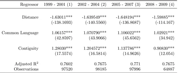
Estimating the trade equations (20) and (21), the results between the two approaches differ in the expected form. Table 1 shows the results of the estimation with the RV
method. Distance, a common language, and a shared border (contiguity) together can
explain about 76% of variation in the data. All coefficients have the expected sign and are economically and statistically highly significant for all years.8 The coefficients on
6
I exclude any overseas territories or departements, Portuguese and Spanish islands in the Atlantic Ocean, Spanish enclaves in Northern Africa, and Gibraltar. See Appendix A for further information.
7
The Nomenclature of Units for Territorial Statistics for European regions classifies by population size: NUTS2, which is used in this paper, is a body of land that is inhabited by a population of size between 800.000 and 3.000.000 and is mainly based on institutional divisions in member states.
8
As annual data has been grouped into four periods of two to three years, standard errors are clustered around importer-exporter pairs. Significance is reported with t-statistics based on cluster-robust standard errors.
Table 1: Trade equation RV Method 1999 - 2009 Regressor 1999 - 2001 (1) 2002 - 2004 (2) 2005 - 2007 (3) 2008 - 2009 (4) Distance -1.63011*** -1.639549*** -1.648194*** -1.59885*** (-138.1693) (-140.5560) (-136.8687) (-114.167) Common Language 1.06157*** 1.070790*** 1.106022*** 1.02921*** (42.8597) (43.9066) (45.6562) (34.942) Contiguity 1.28030*** 1.204572*** 1.137786*** 0.90830*** (17.5574) (16.5814) (14.9626) (12.054) Adjusted R2 0.7602 0.7675 0.771 0.7675 Observations 97520 98185 97996 64887
Note: statistical significance * at p < 0.1, ** at p < 0.05, *** at p < 0.01, cluster-robust t-statistic in
round brackets (standard errors clustered around country pairs). Dependent variable is the logarithm of trade flow, the independent variables are logarithm of distance and binary indicators for a common language and contiguity of countries.
distance are slightly higher for all periods than in Redding & Venables (2004)9 and marginally increase until the fourth period, which is also inline with the literature.10 The importance of contiguity between trading partners is higher than in Redding & Schott (2003) and Redding & Venables (2004) but steadily decreasing. A common language between trading partners, not included in the original Redding & Venables (2004) estimation, displays no particular trend and range marginally lower than the reported values from Breinlich (2006).
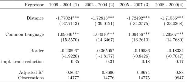
Tables 2 and 3 show the results for the estimation of the trade equation with the HM
method. While all coefficients in both tables have the expected sign, the magnitude
differs tremendously. For all 25 countries of the European Union the coefficient on distance is much larger than for the old member states before the 2004 enlargement, while the border coefficient is much lower for the estimation with all member states compared to the selection of the EU15. This result is somewhat puzzling, as it im-plies much lower trade reductions when crossing a border in the new member state countries compared with the old member states. The issue is most likely rooted in the construction of internal trade data. When exclusively looking at the estimation for the countries that were members of the EU before the enlargement of 2004, the coeffi-cients are to a large extent in line with previous research: the implied trade reductions by crossing a national border mirror Breinlich (2006)’s findings, with values decreas-ing from −72% in the first period to −64% in the third period. Note however that
9Compare (Redding & Venables, 2004, p. 62, Table 1, Column 1) for the same methodology used. 10
See Disdier & Head (2008) for a survey on the topic of the high negative impact of distance on trade.
Table 2: Trade equation HM Method 1999 - 2009 Regressor 1999 - 2001 (1) 2002 - 2004 (2) 2005 - 2007 (3) 2008 - 2009(4) Distance -1.77024*** -1.72813*** -1.72492*** -1.71556*** (-37.7113) (-39.0121) (-34.2575) (-33.0368) Common Language 1.09646*** 1.03010*** 1.09456*** 1.20567*** (15.5570) (14.3467) (16.2610) (14.7680) Border -0.43596* -0.36505* -0.19536 -0.18334 (-1.9220) ( -1.8177) (-0.8426) (-0.7047)
impl. trade reduction 0.35 0.31 0.18 0.17
Adjusted R2 0.8637 0.8696 0.8674 0.88
Observations 14777 14776 14775 9847
Note: statistical significance * at p < 0.1, ** at p < 0.05, *** at p < 0.01, cluster-robust t-statistic in
round brackets (standard errors clustered around country pairs). Dependent variable is the logarithm of trade flow, the independent variables are logarithm of distance and binary indicators for a common language and the crossing of a border. Implied trade reduction is 1− exp(border).
Breinlich (2006) and Head & Mayer (2006) allow border effects to vary across different countries.11 The coefficients are only statistically significant for the first two periods. In both estimations of EU25 and EU15 a common language plays an economically and statistically significant role in the determination of the size of trade flows, although the coefficient varies across time. The estimation of the trade equation with the HM
method explains between 86%− 90% of the variation of trade flows. Although
coeffi-cients vary substantially between the estimations for the EU25 and EU15, to ensure consistency those coefficients of the estimation with all 25 countries of the European Union are used for the calculation of the market access.
In the analysis below, mostly the results from the HM method will be used, as the information on internal trade flows appears to be extraordinarily important in the context of regions, as will be shown below. However, the results from the RV method are overall similar and provide a good contrast to be used to underpin the general findings and highlight the differences rooted in the construction of the two methods.
3.5 Computation of Market Access
Having obtained estimates for trade costs and importer fixed effects, I can proceed to compute the market access for all regions. However, the trade equation, as described above, is estimated with national data. To make the step to regional market access, one
11
Letting border effects vary across countries in my case led to enormous variations in the later calculated market access. I therefore resorted to assuming a common effect, although Chen (2004) finds significant differences for the effect for European countries.
Table 3: Trade equation HM Method 1999 - 2009 for EU15 only Regressor 1999 - 2001 (1) 2002 - 2004 (2) 2005 - 2007 (3) 2008 - 2009 (4) Distance -1.1965275*** -1.203978*** -1.175567*** -1.181475*** (-22.4601) (-23.6480) (-19.0561) (-18.6857) Common Language 1.1780656*** 1.116936*** 1.213514*** 1.284977*** (17.6732) (1.060122) (19.4007) (16.4424) Border -1.2741031* -1.060122* -1.037907 -1.141489 (-6.1237) ( -4.5934) (-4.0140) (-3.8505)
impl. trade reduction -72 % -65 % -64 % -68 %
Adjusted R2 0.8954 0.9003 0.892 0.9059
Observations 8844 8844 8844 5898
Note: statistical significance * at p < 0.1, ** at p < 0.05, *** at p < 0.01, cluster-robust t-statistic in
round brackets (standard errors clustered around country pairs). Dependent variable is the logarithm of trade flow, the independent variables are logarithm of distance and binary indicators for a common language and the crossing of a border. Implied trade reduction is 1− exp(border). Note that this estimation only includes data on EU15 countries.
critical assumption has to be made: all regions in a country share the same price-level. While this assumption is quite strong and disregards apparent differences (Combes
et al. , 2008), it allows to split the estimated importer country fixed effect by regional
expenditure shares: exp(IMs)η2,s = µsYs µSYS exp(IMS) η2,S = µsYs PS1−σ (22)
where region s is situated in the importing country S, implying Ps = PS,∀s ∈ S. The
trade equation is also estimated with national data on trade costs, so for the calculation of region market access, the regional data is used, relying on official regional languages and distances from regions to countries, other regions within the same country and internal distances as described in section 3.3.
Recalling equation (15), the market access will then be calculated using equation (19) accordingly for the respective time t as:
M Ar,t= R ∑ s=1 µs,tYs,tPs,tσ−1τrs,t1−σ = R ∑ s=1 (js,t)(τrs,t1−σ) ⇒ MAr,t= R ∑ s=1 (
exp(IMs)η2,s,t(DISTrs)ζ3,texp(LAN Grs)ζ4,texp(BORDERrs)ζ5,t
) (23)
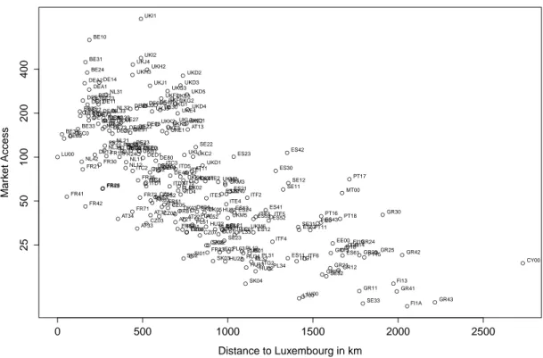
Figure 1: Distance to Luxembourg and Market Access in Period 1999 - 2001 ● ● ● ● ● ● ● ● ● ● ● ● ● ● ● ● ● ● ● ● ● ● ● ● ● ● ● ● ● ● ● ● ● ● ● ● ● ● ● ● ● ● ● ● ● ●● ● ● ● ● ● ● ● ● ●● ● ● ● ● ● ● ● ● ● ● ● ● ● ● ● ● ● ● ● ● ● ● ● ● ● ● ● ● ● ● ● ● ● ● ● ● ● ● ● ● ● ● ● ● ● ● ● ● ● ● ● ● ●● ● ● ● ● ● ● ● ● ● ● ● ● ● ● ● ● ● ● ● ● ● ● ● ● ● ● ● ● ● ● ● ●● ● ● ● ● ● ● ● ● ● ● ● ● ● ● ● ● ● ● ● ● ● ● ● ● ● ● ● ● ● ● ● ● ● ● ● ● ● ● ● ● ● ● ● ● ● ● ● ● ● ● ● ● ● ● ● ● ● ● ● ● ● ● ● ● ● ● ● ● ● ● ● ● ● ● ● ● ● ● ● ● ● ●● ● ● ● ● ● ● ● ● ● ● ● ● ● ● ● ● ●● ● ● ● 0 500 1000 1500 2000 2500 Distance to Luxembourg in km Mar k et Access AT11 AT12 AT13 AT21AT22 AT31 AT32 AT33 AT34 BE10 BE21 BE22 BE23 BE24 BE25 BE31 BE32 BE33 BE34 BE35 CY00 CZ01 CZ02 CZ03 CZ04 CZ05 CZ06 CZ07 CZ08 DE11 DE12 DE13 DE14 DE21 DE22 DE23 DE24 DE25 DE26DE27 DE30 DE41 DE42 DE50DE60 DE71DE72 DE73 DE80 DE91 DE92DE93 DE94 DEA1 DEA2 DEA3 DEA4 DEA5 DEB1 DEB2 DEB3 DEC0 DED1 DED2 DED3 DEE0 DEF0 DEG0 DK01 DK02 DK03DK04DK05 EE00 ES11 ES12 ES13 ES21 ES22 ES23 ES24 ES30 ES41 ES42 ES43 ES51 ES52 ES53 ES61 ES62 FI13 FI18FI19 FI1A FI20 FR10 FR21 FR22 FR23 FR24 FR25 FR26 FR30 FR41 FR42 FR43 FR51 FR52 FR53 FR61FR62 FR63 FR71 FR72 FR81 FR82 FR83 GR11 GR12 GR13GR14 GR21 GR22 GR23 GR24 GR25 GR30 GR41 GR42 GR43 HU10 HU21 HU22 HU23 HU31 HU32 HU33 IE01 IE02 ITC1 ITC2 ITC3 ITC4ITD1 ITD2 ITD3 ITD4 ITD5ITE1 ITE2 ITE3 ITE4 ITF1 ITF2 ITF3 ITF4 ITF5 ITF6 ITG1 ITG2 LT00 LU00 LV00 MT00 NL11 NL12 NL13 NL21 NL22 NL23 NL31 NL32 NL33 NL34 NL41 NL42 PL11 PL12 PL21 PL22 PL31 PL32 PL33 PL34 PL41 PL42 PL43 PL51PL52 PL61 PL62 PL63 PT11 PT15 PT16 PT17 PT18 SE11 SE12 SE21 SE22 SE23 SE31 SE32 SE33 SI01 SI02 SK01 SK02 SK03 SK04 UKC1 UKC2 UKD1 UKD2 UKD3 UKD4 UKD5 UKE1 UKE2 UKE3 UKE4 UKF1 UKF2 UKF3 UKG1UKG2 UKG3 UKH1 UKH2 UKH3 UKI1 UKI2 UKJ1 UKJ2UKJ3 UKJ4 UKK1 UKK2 UKK3 UKK4 UKL1 UKL2 UKM2UKM3 UKM5 UKM6 UKN0 25 50 100 200 400
Note: Distance to Luxembourg in kilometers and market access relative to Luxembourg (LU00 =
100). Market access calculated with HM method for period from 1999 - 2001.
for the HM method and
⇒ MAr,t=
R
∑
s=1
(
exp(IMs)η2,s,t(DISTrs)ζ3,texp(LAN Grs)ζ4,texp(CON T IGrs)ζ5,t
) (24) for the RV method.
Figure 1 displays the resulting market access values of the 248 regions, using coefficients calculated with the HM method, for the period of 1999 - 2001 relative to their distance from Luxembourg. The trend is easily visible: the further a region is located from the geographic center of the European Union the lower is its market access. Particularly well positioned and blessed with a high market access seem to be the metropolitan re-gions of London (NUTS 2 codes UKI1 and UKI2) and Brussels (NUTS 2 codes BE10, BE31 and BE24).12 Of particular interest with respect to the latter part of this paper, section 5, is figure 2. While less clear than the relationship between distance to the ge-ographic center and market access, it appears that regions located far from the center
Figure 2: Distance to Luxembourg and Relative Change in Market Access 1999 - 2009 ● ● ● ● ● ● ● ● ● ● ● ● ● ● ● ● ● ● ● ● ● ● ● ● ● ● ● ● ● ● ● ● ● ● ● ● ● ● ● ● ● ● ● ● ● ● ● ● ● ● ● ● ● ● ● ● ● ● ● ● ● ● ● ● ● ● ● ● ● ● ● ● ● ● ● ● ● ● ● ● ● ● ● ● ● ● ● ● ● ● ● ● ● ● ● ● ● ● ● ● ● ● ● ● ● ● ● ● ● ●● ● ● ● ● ● ● ● ● ● ● ● ● ● ● ● ● ● ● ● ● ● ● ● ● ● ● ● ● ● ● ● ●●● ● ● ● ● ● ● ● ● ● ● ● ● ● ● ● ● ● ● ● ● ● ● ● ● ● ● ● ● ● ● ● ●● ● ● ● ● ● ● ● ● ● ● ● ● ● ● ● ● ● ● ● ●● ● ● ● ● ● ● ● ● ● ● ● ● ● ● ● ● ● ● ● ● ● ●● ● ● ● ● ● ● ● ● ●●● ● ● ● ● ● ● ● ● ● ● ●● ● ● ● 0 500 1000 1500 2000 2500 Distance to Luxembourg in km Change in Mar k et Access AT21 AT22 AT31 AT32 AT33 AT34 BE34 CY00 CZ01 CZ02 CZ03 CZ04 CZ05 CZ06 CZ07 CZ08 EE00 ES11 ES12 ES13 ES24 ES30 ES41 ES43 ES51 ES52 ES53 ES61 ES62 FI13 FI18 FI19 FI1A FI20 FR83 GR11 GR12 GR13 GR14 GR21 GR22 GR23 GR24 GR25 GR30 GR41 GR42 GR43 HU10 HU21 HU22 HU23 HU31HU32 HU33 LT00 LU00 LV00 PL11PL21PL12 PL22 PL31 PL32 PL33 PL34 PL41 PL51 PL52 PL61 PL62 PL63 SE21 SE23 SE31 SE32 SE33 SI01 SI02 SK01 SK02 SK03 SK04 AT11 AT12 AT13 BE10 BE21 BE22 BE23 BE24 BE25 BE31 BE32 BE33 BE35 DE11 DE12 DE13 DE14 DE21 DE22 DE23 DE24 DE25 DE26 DE27 DE30 DE41 DE42 DE50 DE60 DE71DE72DE73
DE80 DE91 DE92 DE93 DE94 DEA1 DEA2 DEA3DEA4 DEA5 DEB1 DEB2 DEB3 DEC0 DED1 DED2 DED3 DEE0 DEF0 DEG0 DK01 DK02 DK03DK04DK05 ES21 ES22 ES23 ES42 FR10 FR21 FR22 FR23 FR24 FR25 FR26 FR30 FR41FR42 FR43 FR51 FR52 FR53 FR61FR62 FR63 FR71 FR72 FR81 FR82 IE01 IE02 ITC1 ITC2 ITC3 ITC4ITD1ITD2 ITD3
ITD4 ITD5ITE1 ITE2 ITE3 ITE4 ITF1 ITF2 ITF3 ITF4 ITF5 ITF6 ITG1 ITG2 MT00 NL11 NL12 NL13 NL21 NL22NL23 NL31NL33NL32 NL34 NL41 NL42 PL42 PL43 PT11 PT15 PT16 PT17 PT18 SE11SE12 SE22 UKC1 UKC2 UKD1 UKD2 UKD3 UKD4 UKD5 UKE1 UKE2 UKE3UKE4 UKF1 UKF2 UKF3 UKG1UKG2 UKG3 UKH1 UKH2 UKH3UKI1UKI2UKJ1
UKJ2 UKJ3 UKJ4 UKK1 UKK2 UKK3 UKK4 UKL1 UKL2 UKM2UKM3 UKM5 UKM6 UKN0 −30 −20 −10 0 10 20 30
Note: Distance to Luxembourg in kilometers and change in market access from period 1999 - 2001 to
period 2008 - 2009, relative to Luxembourg. Market access calculated with HM method.
improved their market access in the period of 2008 - 2009 relative to their initial market access in the period of 1999 - 2001 more than those regions located closer to the center.
The differences between the two techniques used to estimate the trade equation become apparent when looking at table 4. Market access calculated based upon coefficients from the RV method is muss less reliant on the domestic component of trade, while the corresponding figures for the HM method mirror the home bias in trade, with respect to both domestic region and country, captured by the border dummy in the estimation. Note also that the latter shows a clear trend for European regions in the composition of their market access: Europe and the rest of the world gain shares at the expense of the domestic region and country. In the RV method no such clear trend is visible, and while the order of importance is equivalent to the HM method, it seems to deliver less precise results.
Table 4: Composition of Market Access for all period using HM method and RV method HM method ’99 - ’01 ’02 - ’04 ’05 - ’07 ’08 - ’09 Region 12.36 11.88 11.53 11.63 Country 70.31 67.76 65.36 65.03 Europe 14.21 16.52 18.62 18.53 World 3.12 3.84 4.49 4.81 RV method ’99 - ’01 ’02 - ’04 ’05 - ’07 ’08 - ’09 Region 7.92 8.19 8.21 7.93 Country 51.56 53.53 52.62 52.11 Europe 38.30 36.25 36.93 37.24 World 2.23 2.03 2.24 2.72
Note: Market access in top half calculated with the HM method, in bottom half calculated with RV
method. Cells show average share of regional, national, European and worldwide component in market access for all 248 regions per time period.
4
Estimation of the Wage Equation
Having obtained estimates for market access, I can proceed to apply these values in the estimation of the wage equation (16) and the related change in wages (17). Recalling from section 2 the wage equation (16) reads:
wr= (c a ) 1 ασ x− β α r M A 1 ασ r
Taking logs and applying a time dimension yields ln wr,t= 1 ασln ( ct at ) −β αln xr,t+ 1 ασM Ar,t
Recall that atcan vary over time but is invariant across regions. This is then estimated
as
ln wr,t= θt+
1
ασln M Ar,t+ ϵr,t (25)
The renumeration for the mobile input, xr,t, is captured in the error term, while the
constant θt captures the time-variant atand ct. All cross-regional differences are thus
assumed to be captured in the residual, which is a quite strong hypothesis (Redding & Venables, 2004). In section 4.2 I therefore conduct several robustness tests.
Wages, the remuneration for the immobile factor, is proxied with GDP per capita, following numerous related papers. As I am calculating the market access over periods, I also take the mean GDP per capita for the respective time periods. Regional GDP data comes from EUROSTAT.
4.1 Baseline Estimation
Table 5: Baseline estimation wage equation 1999 - 2009
Regressor ln(GDPpc) (1) ln(GDPpc) (2) ln(GDPpc) (3) ln(GDPpc) (4) ln(MA RV) 0.25744*** (17.1927) ln(MA HM) 0.345281*** (18.9450) ln(MA) P1 0.30239*** 0.38873*** (9.4554) (10.7178) ln(MA) P2 0.267724*** 0.35773*** (8.6643) (9.6623) ln(MA) P3 0.237804*** 0.32963*** (8.4723) (9.3684) ln(MA) P4 0.212776*** 0.28435*** (7.9523) (8.2021)
Period Dummies yes yes yes yes
Adjusted R2 0.2702 0.2965 0.2722 0.2978
Observations 992 992 992 992
Year 1999 - 2009 1999 - 2009 1999 - 2009 1999 - 2009
Note: statistical significance * at p < 0.1, ** at p < 0.05, *** at p < 0.01, t-statistic in round
brackets. Due to the nature of the regressor being itself generated from a prior regression, t-statistics should be reported based on bootstrapped standard errors, which however could not be done. The independent variable is the logarithm of the mean of GDP per capita in the respective period, as described in the text. The regressors in columns (1) and (2) are the logarithms of the market access calculated with the RV method in column (1) and HM method in column (2). The regressors in columns (3) and (4) are the logarithm of the market access in period 1 (P1 = 1999 - 2001), period 2 (P2 = 2002 - 2004), period 3 (P3 = 2005 - 2007) and period 4 (P4 = 2008 - 2009) calculated with the RV method in column (3) and the HM method in column (4).
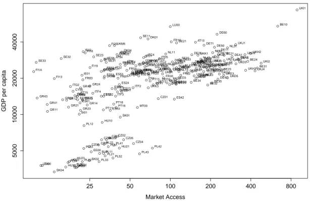
Table 5 reports the results for the baseline estimation using both above described methods. Market access is in all cases economically and statistically highly significant and the estimated coefficients are well in line with the results from the directly related research, Breinlich (2006) and Head & Mayer (2006) in particular. Making use of the panel character of the data, columns (1) and (2) report the average impact of market access on wages, with market access calculated with the RV method and HM method respectively. Columns (3) and (4) allow the coefficient to vary by period. In both specifications, the impact of market access decreases. Figure 3 plots the relationship for the period of 1999 -2001. To a large part the downward trend of the coefficient is due to the upward movement of the distinct group of points in the lower left of
Figure 3: GDP per capita and Market Access in 1999 - 2001 ● ● ● ●● ● ● ● ● ● ● ● ● ● ● ● ● ● ● ● ● ● ● ● ● ● ● ● ● ● ● ● ● ● ● ● ● ● ●● ● ● ● ● ● ● ● ● ● ●● ● ● ● ● ● ● ● ● ● ● ● ● ● ● ● ● ● ● ● ●● ● ● ● ● ● ● ● ● ● ● ● ● ● ● ● ● ● ● ● ● ● ● ● ● ● ● ● ● ● ● ● ● ● ● ● ● ● ● ● ● ● ● ● ● ● ● ● ● ● ● ● ● ● ● ● ● ● ● ● ● ● ● ● ● ● ● ● ● ● ● ● ● ● ● ● ● ● ● ● ● ● ● ● ● ● ● ● ● ● ● ● ● ● ● ● ● ● ● ● ● ● ● ● ● ● ● ● ● ● ● ● ● ● ● ● ● ● ● ● ● ● ● ● ● ● ● ● ● ● ● ● ● ● ● ● ● ● ● ● ● ● ● ● ● ● ● ● ● ● ● ● ● ● ● ● ● ● ● ● ● ● ● ● ● ● ● ● ● ● ● ● ● ● ● ● ● Market Access GDP per capita AT11 AT12 AT13 AT21AT22 AT31 AT32 AT33 AT34 BE10 BE21 BE22 BE23 BE24 BE25 BE31 BE32 BE33 BE34 BE35 CY00 CZ01 CZ02 CZ03 CZ04 CZ05 CZ06 CZ07 CZ08 DE11 DE12 DE13 DE14 DE21 DE22 DE23 DE24 DE25 DE26DE27 DE30 DE41 DE42 DE50 DE60 DE71 DE72 DE73 DE80 DE91DE92 DE93 DE94 DEA1 DEA2 DEA3 DEA4 DEA5 DEB1 DEB2 DEB3 DEC0 DED1 DED2 DED3 DEE0 DEF0 DEG0 DK01 DK02 DK03DK04 DK05 EE00 ES11 ES12 ES13 ES21 ES22 ES23 ES24 ES30 ES41 ES42 ES43 ES51 ES52 ES53 ES61 ES62 FI13 FI18 FI19 FI1A FI20 FR10 FR21 FR22 FR23 FR24 FR25 FR26 FR30 FR41 FR42 FR43 FR51 FR52 FR53 FR61 FR62 FR63 FR71 FR72 FR81 FR82 FR83 GR11 GR12 GR13 GR14 GR21 GR22 GR23 GR24 GR25 GR30 GR41 GR42 GR43 HU10 HU21 HU22 HU23 HU31 HU32 HU33 IE01 IE02 ITC1 ITC2 ITC3 ITC4 ITD1 ITD2 ITD3 ITD4 ITD5 ITE1 ITE2 ITE3 ITE4 ITF1 ITF2 ITF3 ITF4 ITF5 ITF6 ITG1 ITG2 LT00 LU00 LV00 MT00 NL11 NL12 NL13NL21 NL22 NL23 NL31 NL32 NL33 NL34 NL41 NL42 PL11 PL12 PL21 PL22 PL31 PL32 PL33 PL34 PL41 PL42 PL43 PL51 PL52 PL61 PL62 PL63 PT11 PT15 PT16 PT17 PT18 SE11 SE12 SE21 SE22 SE23 SE31 SE32 SE33 SI01 SI02 SK01 SK02 SK03 SK04 UKC1 UKC2 UKD1 UKD2 UKD3 UKD4 UKD5 UKE1 UKE2 UKE3 UKE4 UKF1 UKF2 UKF3 UKG1 UKG2 UKG3 UKH1 UKH2 UKH3 UKI1 UKI2 UKJ1 UKJ2 UKJ3 UKJ4 UKK1 UKK2 UKK3 UKK4 UKL1 UKL2 UKM2 UKM3 UKM5 UKM6 UKN0 5000 10000 20000 40000 25 50 100 200 400 800
Note: Average GDP per capita in 1999 - 2001 (2010 EURO) and the regions’ market access (LU00 =
100) in 1999 - 2001.
the graph - almost exclusively regions located in the new member states entering the European Union in 2004.13 The estimated values range between 0.21− 0.3 for the RV method and 0.28− 0.38 for the HM method, implying an average increase in GDP per
capita between 21%− 30% and 28% − 38% respectively for a doubling of the value of market access, depending on the time period and method used. Market access explains between 27%− 30% of the variation of income. The implied values for σ, the elasticity of substitution, are plausible as well, when assuming a standard α = 23: they range in between 7.04 and 3.85.
The determination of wages by market access of a region may appear well established through the results, however the attention should be turned to two important issues: First, the use of GDP data, or the estimation of it as through the trade equation, creates an immediate endogeneity problem for the wage equation, where GDP per capita, as a proxy for wages, is regressed on market access. Second, as Redding & Venables (2004) and Breinlich (2006) point out, the returns on the mobile input should equalize across countries and regions by assumption, and would therefore be captured in the constant not the error term, which would create another source of endogeneity.
13
See table 11 for the corresponding baseline estimation for only EU15 regions and figure 6 for the plot in the period of 2008 - 2009 in appendix C.
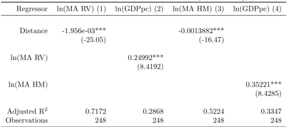
Table 6: Instrumental Variable Estimation (1999 - 2001)
Regressor ln(MA RV) (1) ln(GDPpc) (2) ln(MA HM) (3) ln(GDPpc) (4)
Distance -1.956e-03*** -0.0013882*** (-25.05) (-16.47) ln(MA RV) 0.24992*** (8.4192) ln(MA HM) 0.35221*** (8.4285) Adjusted R2 0.7172 0.2868 0.5224 0.3347 Observations 248 248 248 248
Note: statistical significance * at p < 0.1, ** at p < 0.05, *** at p < 0.01. t-statistic in round
brackets based on heteroskedasticity-robust standard errors. Due to the nature of the regressor in columns (2) and (4) being itself generated from a prior regression, t-statistics should also be reported based on bootstrapped standard errors, which however could not be done. ln(MA XY) is the logarithm of the market access in the period 1999 - 2001 calculated with the respective method.
4.2 Robustness Checks
It is apparent that by construction of the market access variable one should be con-cerned about endogeneity. The domestic component, even when not explicitly calcu-lated, as in the RV method, shows the local expenditure on the considered good. This expenditure is dependent on the income, which itself is of course dependent on the wage, the dependent variable of the estimation, creating a potential reverse causality. As Head & Mayer (2004) note, in the extreme case where transport costs are infinitely high, only local expenditure enters the market access. Redding & Venables (2004) address this concern with excluding the domestic component from the estimation and regressing wages exclusively on what they call foreign market access. This in turn however eliminates the arguably most important source of high wages, in particular where market access is high: the demand from the own region. Exemplifying this by taking the Belgium capital region Brussels (NUTS2 code BE10), market access cal-culated with the HM method for the period of 1999 - 2001 is reduced by 53% when excluding the domestic region, while at the same time, the neighboring regions Flem-ish Brabant (NUTS code BE24) and Walloon Brabant (NUTS code BE31) lose only 5% and 3% respectively, as they draw most of their total market access not from the own region, but from the capital region of Brussels, which is still included in their exclusively non-domestic market access.14
Another approach to solve the simultaneity problem is to find a good instrument
14
This also becomes apparent in table 4, as described above, showing the shares in market access for domestic region, country, Europe and the rest of the world.
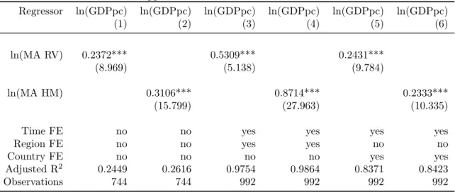
Table 7: Lagged Market Access and Fixed Effects Regressor ln(GDPpc) ln(GDPpc) ln(GDPpc) ln(GDPpc) ln(GDPpc) ln(GDPpc) (1) (2) (3) (4) (5) (6) ln(MA RV) 0.2372*** 0.5309*** 0.2431*** (8.969) (5.138) (9.784) ln(MA HM) 0.3106*** 0.8714*** 0.2333*** (15.799) (27.963) (10.335)
Time FE no no yes yes yes yes
Region FE no no yes yes no no
Country FE no no no no yes yes
Adjusted R2 0.2449 0.2616 0.9754 0.9864 0.8371 0.8423
Observations 744 744 992 992 992 992
Note: statistical significance * at p < 0.1, ** at p < 0.05, *** at p < 0.01. t-statistic in round
brackets based on heteroskedasticity-robust standard errors. Due to the nature of the regressor being itself generated from a prior regression, t-statistics should also be reported based on bootstrapped standard errors, which however could not be done. ln(MA XY) is the logarithm of the market access calculated with the respective method. The dependent variable is the logarithm of GDP per capita, average per period lagged by one period in columns (1) and (2), and average for the period for columns (3) to (6). Estimations for column (3) and (4) include time and region fixed effects, for column (5) and (6) include time and country fixed effects. Coefficients for all time, region and country fixed effects are not reported.
that is not influenced by wages, but is highly correlated with the calculated market access. As figure 1 shows, the distance to Luxembourg appears to qualify well for this task as a purely geographical variable.15 Table 6 shows the results for the IV estimation for the period of 1999 - 2001: in the first stage, distance, as the instrumental variable already explains 71% and 52% respectively of variation in regional market access (column 1 for RV method and column (2) for HM method ). In the second stage, the coefficients in columns (2) and (4) are slightly smaller, but they remain highly economically significant and hence very similar in magnitude and are just as significant statistically as in the baseline estimation.
However also the non-domestic component raises concerns: as Breinlich (2006) notes, shocks to wages may be spatially correlated, such as a nationwide strike. To control for such effects, I estimate the same baseline regression with a one-period lag (Table 7, columns (1) and (2)). Country-specific effects that are time-persistent, e.g. insti-tutional setting, can be controlled for by including a country fixed effect (Table 7, columns (5) and (6)). Other unobserved variables may be region-specific and
time-15Breinlich (2006) includes a second instrument, country size, to account for a large national market
in the light of border effects. In my analysis such measure is insignificant for EU25, but vagely significant for EU15. Regional size is highly significant with a negative sign, however the endogeneity here is clear: administrative regions are man-made smaller in metropolitan areas because of higher population in a smaller area, where income, and hence market access is higher.
persistent (Table 7, columns (5) and (6)). None of these fixed effects or lagged variables reduce the significance of market access for the determination of wages.16 All controls for robustness underline the importance of market access in the determination of the remuneration for the immobile factor.
5
The Role of EU Funds
The European Union Regional Policy, as briefly characterized in section 1, aims to promote cohesion among European regions in economic, social and territorial terms. The means to achieve these forms of cohesion are specified in the objectives, and I here focus on Objective 1 and the Cohesion Fund, and Objective 2. The theoretical and econometric framework setup in the previous sections allow to analyze, whether these two objectives have achieved a measurable effect, as they are directly concerned with economic prosperity.
To evaluate the success of this aim in the proposed theoretical framework in section 2, I now analyze the change in wages, as postulated in equation (17).
5.1 Change in Wages
The estimation of the change in wages, is expectedly similar to the estimation of the wage equation (25) in section 4. Recalling equation (17) from section 2:
∆ ln wr,t= 1 ασ(∆ ln ct− ∆ ln at)− β α∆ ln xr,t+ 1 ασ∆ ln M Ar,t
This is estimated analogous equation to (25) as ln wr,t− ln wr,t−1 = θt+
1
ασ(ln M Ar,t− ln MAr,t−1) + ϵr,t (26)
Again θt captures the time-variant at and at−1 as well as a change in the elasticity
of substitution ct. The return on the mobile factor, xr,t and xr,t−1 is captured in the
error term ϵr,t.17
In section 5.2 I first estimate equation (26) and control for initial GDP and the change of human capital. Afterwards in section 5.3 I inspect with the estimation of equation (27) whether and how funds from the EU regional policy facilities influenced the change in wages and interacted through the assumed channels.
16While the value for the coefficient shoots up when introducing a regional fixed effect (Columns
(3) and (4)), in both cases the intercept, not displayed in the table, also drops significantly. The coefficients have no economic interpretation, only their significance is important.
17
The same possibility of it being captured in the constant as in the equation (25) remains. See section 4.2 for robustness tests in this respect.
Figure 4: Change of Market Access (HM method) and Change in GDP 1999 - 2009 ● ● ● ● ● ● ●● ● ● ● ● ● ● ● ● ● ● ● ● ● ● ● ● ● ● ● ● ● ● ● ● ● ● ● ● ● ● ● ● ● ● ● ● ● ● ● ● ● ● ● ● ● ● ● ● ● ●● ● ● ● ● ● ● ● ● ● ● ● ●● ● ● ● ● ● ● ● ● ● ● ● ● ● ● ● ● ● ● ● ● ● ● ● ● ● ● ●●●● ● ●● ● ● ● ● ●● ● ● ● ● ● ● ● ● ● ● ● ● ● ● ● ● ● ● ● ● ● ● ● ●● ● ● ● ● ● ● ● ● ● ● ● ● ● ● ● ● ● ● ● ● ● ●● ● ● ● ● ● ● ● ● ● ● ● ● ● ● ● ● ● ●● ● ● ● ● ● ● ● ● ● ● ● ● ● ● ● ● ● ● ● ● ● ● ● ● ● ● ● ● ● ● ● ● ● ● ● ● ● ● ● ● ● ● ● ● ● ● ● ● ● ● ● ● ● ● ● ● ● ● ● ● ● ● ● ● ● ● ● ● ● ● −40 −20 0 20 −20 0 20 40 60 80 100
Change of Market Access in %
Change of GDP per capita in %
AT21 AT22 AT31 AT32AT33AT34 BE34 CY00 CZ01 CZ02 CZ03 CZ04 CZ05 CZ06 CZ07 CZ08 EE00 ES11 ES12 ES13ES24 ES30 ES41 ES43 ES51 ES52 ES53 ES61 ES62 FI13 FI18 FI19 FI1A FI20 FR83 GR11 GR12 GR13 GR14 GR21 GR22 GR23 GR24 GR25 GR30 GR41 GR42 GR43 HU10 HU21 HU22 HU23 HU31HU32 HU33 LT00 LU00 LV00 PL11PL12 PL21 PL22 PL31 PL32 PL33 PL34 PL41 PL51 PL52 PL61 PL62 PL63 SE21SE23 SE31 SE32 SE33 SI01 SI02 SK01 SK02 SK03 SK04 AT11 AT12 AT13 BE10 BE21 BE22 BE23 BE24 BE25 BE31 BE32 BE33 BE35 DE11 DE12 DE13 DE14 DE21 DE22 DE23 DE24 DE25 DE26 DE27 DE30 DE41 DE42 DE50 DE60 DE71 DE72 DE73 DE80 DE91 DE92 DE93 DE94 DEA1 DEA2 DEA3 DEA4 DEA5DEB1 DEB2 DEB3 DEC0 DED1 DED2 DED3 DEE0 DEF0 DEG0 DK01 DK02 DK03DK04 DK05 ES21 ES22 ES23 ES42 FR10 FR21 FR22 FR23FR24FR25FR26 FR30 FR41FR42 FR43 FR51 FR52FR53 FR61FR62 FR63 FR71 FR72 FR81 FR82 IE01 IE02 ITC1 ITC2 ITC3 ITC4 ITD1 ITD2ITD3 ITD4 ITD5ITE1ITE2
ITE3 ITE4 ITF1 ITF2 ITF3 ITF4 ITF5 ITF6ITG1 ITG2 MT00 NL11 NL12 NL13 NL21 NL22 NL23 NL31 NL32NL33 NL34 NL41 NL42 PL42 PL43 PT11 PT15 PT16 PT17 PT18 SE11 SE12 SE22 UKD1 UKI1 UKJ3 UKK3 UKM5UKM6 UKC1 UKC2 UKD2UKD3 UKD4
UKD5 UKE1 UKE2 UKE3 UKE4 UKF1 UKF2 UKF3 UKG1 UKG2 UKG3 UKH1 UKH2 UKH3 UKI2 UKJ1 UKJ2 UKJ4 UKK1 UKK2 UKK4 UKL1 UKL2 UKM2UKM3 UKN0
Note: Distance to Luxembourg in kilometers and market access relative to Luxembourg (LU00 =
100). Market access calculated with HM method for period from 1999 - 2001.
Data for the EU Regional Funds comes from (Gallo et al. , 2011; Dall’erba & Le Gallo, 2008, 2007; Dall’erba, 2005) and EU DG Regio. I follow Lopez-Rodriguez et al. (2007) in proxying human capital with by the share of the population aged 25 - 59 (aged 25-64 for 2008) with an educational attainment of at least upper secondary education.18
5.2 Baseline Estimation of Change in Wages
Columns (1), (2) and (3) of table 8 report the results for the baseline estimation of the change in wages. Column (1) shows that on average for all 248 regions a doubling of the market access over the entire time period from 1999 - 2009 resulted on average in an increase in GDP per capita of 90%. Columns (2) and (3) allow the coefficient to vary between old and new member states, and Objective 1 and 2 regions respectively. The result is revealing: while in the old member states a doubling of the market access of a region resulted in an increase of GDP per capita of only 63%, for new member states it yielded a massive 147%.
18
Unfortunately data for Denmark, Sweden, Slovenia and the UK Highlands is uncomplete due to a change in NUTS2 regions.
T able 8: Baseline estimation of Change in W ages (HM metho d, 1999 -2009), Con trols for Initial GDP p er capita and Change in Human Capital ∆ln(GDPp c) ∆ln(GDPp c) ∆ln(GDPp c) ∆ln(GDPp c) ∆ln(GDPp c) ∆ln(GDPp c) ∆ln(GDPp c) ∆ln(GDPp c) ∆ln(GDPp c) Regressor (1) (2) (3) (4) (5) (6) (7) (8) (9) ∆ln(MA) 0.9073*** 0.7291*** 0.801*** (18.148) (13.3132) (13.3429) ∆ln(MA) EU15 0.6280*** 0.5613*** 0.6402*** (17.6838) (13.1776) (14.8634) ∆ln(MA) EU+10 1.46556*** 1.289*** 0.3461 (4.9644) (4.9688) (0.538) ∆ln(MA) OBJ1 0.9781*** 0.9061*** 0.9359*** (13.1154) (10.5078) (10.2015) ∆ln(MA) OBJ2 0.7004*** 0.6667*** 0.5423*** (7.2472) (7.7660) (10.6290) initial GDPp c -5.7e-06*** -3.6e-06*** -2.89e-06 -1.9e-06 1.02e-06 5.31e-07 (-3.7895) (-3.692) (-1.4957) (-1.4248) (1.113) (0.5195) ∆HC -0.04061 (-0.1405) ∆HC EU15 0.7145** (3.0816) ∆HC EU+10 0.914 (0.617) ∆HC OBJ1 -0.5676 (-1.0546) ∆HC OBJ2 0.8769** (3.2211) EU15 dumm y no y es no no y es no no y es no Ob j. 1 dumm y no no y es no no y es no no y es Adjusted R 2 0.6455 0.7197 0.7101 0.687 0.7335 0.7151 0.7072 0.8168 0.7426 Observ ations 248 248 231 248 248 231 166 166 166 Note: statistical significance * at p < 0 .1, ** at p < 0 .05, *** at p < 0 .01, t-statistic in round brac k ets. Due to the nature of the regressor b eing itself generated from a prior regression, t-statistics should b e rep orted based on b o otstrapp ed standard errors, whic h ho w ev er could not b e done. The indep enden t v ariable is the first difference of the logarithm of GDP p er capita, as describ ed in the text. The regressors are the difference of the logarithm of Mark et Access calculated with the HM metho d, initial GDP p er capita, the difference of Human Capital. All differences b et w een the p erio d of 1999 -2001 and 2008 -2009. EU15 signals the group of old mem b er states, EU+10 the group of new mem b er states after the enlargemen t of the EU in 2004. OBJ1 and OB2 group b y recipien t region of Ob jectiv e 1 and 2 funds from Regional P olicy .
A similar picture is painted when differentiating between Objective 1 and 2 regions:19
an improvement of market access by 100% for the former yielded a 98% increase in GDP per capita, while it was only 70% for an Objective 2 region. The results hint at the higher impact of market access improvement for lesser developed regions. Figure 4 displays this relationship graphically.
To further establish this relationship, columns (4) to (9) of table 8 control for two standard controls in growth regressions, the change in human capital over the same time period and the initial GDP per capita, as classical growth theory predicts higher growth rates for initially poorer regions.20 Only controlling for initial GDP expectedly lowers the coefficients in all three specifications, columns (4), (5) and (6), but all remain highly significant. Additionally controlling for the change in human capital shows interesting results, in particular for the specification splitting between Objective 1 and 2 regions in column (9): while market access retains an economic and statistical significance for both groups, the change in human capital is only statistically significant for Objective 2 regions. A 10% increase in human capital in an Objective 2 region yielded on average an increase of 8.8% in GDP per capita. The increase of market access for comparison by 10% yielded only an increase by 5.4% in an Objective 2 region, while boosting GDP per capita in an Objective 1 region by 9.4%. The explained variation of the change in wages varies between 65%− 82%.
5.3 Estimation of the Effect of Regional Policy Funds
In the light of these results it is interesting to see whether financial flows from the respective Objective 1 and 2, and Cohesion funds in the programming period of 2000 - 2006 had an influence on the change of wages over the time period of 1999 to 2009. To estimate this effect I come back to equation (26). The impact of funds from the regional policy can then be estimated with
ln wr,t− ln wr,t−1 = θt+
1
ασ(ln M Ar,t− ln MAr,t−1) + HrEUr+ ϵr,t (27)
where EUr is a vector of the different funding sources and Hr a vector of possible
interaction channels.
As previously discussed, Objective 1 and the Cohesion Fund have the aim to allow poorer regions to converge, having a primary focus on the financing of infrastructure
19
Note that, as explained in section 1 Objective 1 regions are comprised of almost all new mem-ber state regions, except for Prague, Bratislava and Cyprus, and a smaller nummem-ber from peripheral countries. The similarity in the direction of the coefficients in columns (2) and (3) is therefore no surprise.
20
See Mankiw et al. (1992) for the seminal work including human capital in a standard neoclassical Solow-Swan model.