Chattering-free Sliding Mode Control for Propellantless Rendez-vous using Differential Drag

CHATTERING-FREE SLIDING MODE CONTROL FOR PROPELLANTLESS

RENDEZ-VOUS USING DIFFERENTIAL DRAG

Hancheol Cho, Lamberto Dell’Elce, Gaëtan Kerschen

University of Liège, Space Structures & Systems Laboratory,

1, Chemin des Chevreuils, Liège B-4000, Belgium, Tel.: +32 4366 9449,

hancheol.cho@ulg.ac.be, lamberto.dellelce@ulg.ac.be, g.kerschen@ulg.ac.be

ABSTRACT

This paper develops a differential drag-based sliding mode controller for satellite rendez-vous. It is chattering-free and avoids bang-bang type control to adjust the relative motion more efficiently. In spite of uncertain nonlinear perturbations and disturbances, it is shown that the in-plane relative motion between two satellites can be effectively controlled by regulating the drag difference. An adaptive tuning rule is also presented such that the errors are suppressed to lie within a desired error box. The proposed controller is simple and easy to implement in a small satellite, and numerical simulations are carried out to demonstrate its effectiveness in a high fidelity environment.

Index Terms— Rendez-vous, Differential drag,

Adaptive sliding mode control, Chattering 1. INTRODUCTION

Owing to the well-established correlation between spacecraft mass and mission’s cost, there is great interest in fuel-optimal relative maneuvers between two or more satellites. In this context, the exploitation of natural perturbations is an attractive means to reduce or even remove fuel consumption, and hence, propellantless maneuvers using solar sail [1], geomagnetic field [2], Coulomb forces [3], and atmospheric drag were proposed. Amongst them, the idea to use differential drag as control force for relative motion is particularly attractive to enhance the maneuverability of small satellites in low-Earth orbit, so that ongoing and forthcoming missions envisage this technique to achieve propellantless rendez-vous, cluster keeping, or constellation deployment, e.g., QARMAN [4], SAMSON [5], and Flock [6], respectively. The utilization of differential drag to control the relative motion of satellites was first proposed by Leonard [7]. Based on the linearized Hill-Clohessy-Wiltshire equations [8,9], a rendez-vous strategy was proposed in which the relative motion of the chaser around the target is decomposed into a mean and a harmonic component, which inspired numerous researchers thereafter [10-12]. Bevilacqua et al. [13] used a similar approach to include the secular effects of the second zonal

harmonic (J2) perturbation. They further devised an adaptive Lyapunov-based controller with bang-bang type to account for nonlinear unmodeled dynamics [14]. In [15], a simple proportional-integral-derivative controller was derived to maintain the along-track distance between the two satellites using differential drag. Since bang-bang control cannot easily be implemented in practice, Dell’Elce and Kerschen [16] developed a non bang-bang optimal controller via model predictive control and compared it with an existing analytical technique.

In this paper a new chattering-free sliding mode controller is developed to perform an optimal rendez-vous of two satellites in low-Earth orbit, exploiting differential drag as control force. The proposed controller is designed to successfully compensate for uncertainty effects and/or unmodeled dynamics associated with air drag and to account for practical limitations such as input saturation. Also, continuity of the control functions embedded in the controller guarantees no chattering, hence, non bang-bang type control is obtained. In addition, a simple adaptive law to accurately estimate uncertainty bounds and a control gain is introduced. The novel sliding mode controller with the adaptive law automatically updates the control gain in real time to have errors remain within a user-specified small region. Numerical simulations assuming a realistic scenario are used to validate the robustness and accuracy of the chattering-free sliding mode controller.

2. RENDEZ-VOUS USING DIFFERENTIAL DRAG In the current paper, it is assumed that only in-plane control is considered for rendez-vous. It is known that the controllability of the differential drag in the out-of-plane direction is two orders of magnitude smaller even for highly inclined orbits [17], and hence, it is quite limited to control the out-of-plane motion solely using differential drag. The main purpose of this paper is to develop a computationally

simple and light controller that is able to execute accurate non bang-bang type control for differential drag-based

rendez-vous with low computational overhead, without knowing any information about uncertainties under which the satellites may experience.

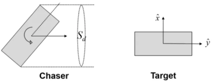
Figure 1 Scheme of attitude motion of chaser and target Let us consider the rendez-vous problem illustrated in Figure 1. The target is assumed to have a stable attitude, while the chaser is controlled in real time by rotating about its orbital plane. The control output is S , the cross-d

sectional area of the chaser exposed to the atmosphere, and it is assumed that the drag of the chaser is proportional to

d

S which is bounded by Sd



Smin,Smax



. A set of the input to the controller comprises

1) estimates for the drag force and its uncertainty bounds obtained by the module ‘drag estimator’ and 2) a reference trajectory computed by the module ‘optimal maneuver planner’,

and both 1) and 2) are evaluated once at the beginning of the maneuver. In this paper, 1) and 2) obtained in [16] are employed to design a sliding mode controller which shall be developed in Section 3.

The ‘drag estimator’ module undertakes the estimation of the drag force on the target and the chaser. The estimation is performed so that it minimizes the mean square errors between the observed and simulated semi-major axes of the satellites. Then, the differential drag is represented by [16]







,c , , , , , , , 1 1 1 , est d est est est

d d t d c d t est d t est d c d est d t est h b t c F F F F F F C S F c x C m       _  _               

where S is the cross-sectional area of the chaser illustrated _d

in Figure 1, m is the mass of the chaser, _c est_, d t

F is the estimated time history of the drag of the target, ,

est d c C is the estimated drag of the chaser, ,

est b t

C is the estimated ballistic coefficient of the target, c is the altitude correction factor, h

and x is the altitude gap between the target and the chaser.

The output ( , est b t C , , est d c C , , est d t

F , c ) of this module serves as h

the input to the ‘optimal maneuver planner’ and the sliding mode controller.

Next, the module ‘optimal maneuver planner’ computes the reference control output ( Sd r, ) and the reference

trajectory ( x y x yr, r,  ) which are solved with an hp-r, r

adaptive Radau pseudospectral transcription [18] using the software GPOPS. To best balance between accuracy and computational efficiency, two dominant perturbations are included in this module: secular J2 effects and short period / altitude-dependent variations of the drag.

It is noted that the coordinate system considered in this paper is the decomposed curvilinear system



x y,



, which considerably improves the accuracy of the solution for middle and long range maneuvers. More specifically, x and

y denote the radial and along-track position of the chaser

with respect to the target, respectively, each of which comprises a mean



x_m,y_m



and an oscillatory component



x y_o, _o



so that xmxox and ymyoy. Schweighart

and Sedwick [19] decomposed into these two components to account for the secular variations of the J2 perturbations. More specifically, the two components satisfy the relations [16]: 

















2 2 2 2 2 2 4 2 , 2 2 2 , 2 2 ₂ , 2 2 2 , m m o o d o o c c x x y c c c y y x c c _c x y F c c y cx                         

where  is the orbital frequency of the target,

 

2 2 2 3 1 1 3cos 2 8 e t t J R c i r   _  _{ is the Schweighart-Sedwick} coefficient, while J2 is the second zonal harmonic coefficient, R is the equatorial radius of the Earth, e r is the t

distance from the center of the Earth to the target, and i is t

the inclination of the reference orbit of the target. The output (Sd r, ,x y x yr, r,  ) of this module then serves as an r, r

input to the controller.

3. CONTROLLER DESIGN

First, consider the ideal (reference) system on which the optimal reference control output (Sd r, ) and the reference

trajectory (x y x yr, r,  ) are derived by the module ‘optimal r, r

/ altitude-dependent variations of the drag are included, the following linearized equation of relative motion [19] holds:







2 , 2 5 2 , 2 , r r r r r d r x cy c x y cx F                

where Fd r, is obtained by (1) and further rewritten using a

normalized control u by _r  , ,





, , , 1 1 , est d c d r est d r d t est h r r r r b t c C S F F c x u C m                

where the normalized control u is bounded by r u r



0,1



.

Next, we consider the real system that is assumed to be expressed in the form of







2 2 5 2 , 2 , x d y x cy c x g y cx F g                  

where g_xg_x



t x y x y, , , , 



and g_yg_y



t x y x y, , , , 



are

unknown perturbations and disturbances that compensate for any differences between the left hand sides and the right

hand sides in (5). In addition, Fd is given in (1) and

further rewritten in the form:















, , , 1 1 , est d c d est d d t est h b t c r r C S F F c x C m u         _   _            

where  and  are uncertain additional terms, and

 

0,1

u  .

Then, the error dynamics is described by











2 2 5 2 , 2 , x y x x y x r y e ce c e g e ce u u g                         

where e_xxx_r , e_y yy_r,   u u u_r, and the terms

x

g and



     u  gy



are uncertain. The aim is to

develop a control law u so that, upon applying it, the errors e and x e converge to zero while suppressing the y

effects of the uncertainties. It should be noted that the control output u for the real system is given by uu_r  . u

Now, define the 2-vector sliding surface s_{ }s_x s_y_ T of the form:  s e Se,   where e_{ }e_x e_y_{ and} T 



2



2 2 2 2 _, 2 2 0 c c c c S      _         _     

where  is a positive small constant. In order to guarantee

the asymptotic stability, the real part of the eigenvalues of

S should be negative, which is equivalent to the condition 0   . When s 0, (8) yields 



2



2 2 2 2 , 2 2 . x y x y x c e e c e c e ce              

From (2), the errors on the mean components of the trajectory satisfy 









2 , 2 2 , 2 4 2 , 2 2 2 , 2 x m x y y m y x c c e e e c c c e e e c             

and if we substitute (10) into (11), we find that the mean component errors become

 , , ₂ 0, 4 . 2 x m y m x e c e e c      

Hence, if we choose a sufficiently small value for  , the

mean component errors are identically zero in the x direction and very small in the y direction. Furthermore, (10) is analogous to the dynamics of the errors on the oscillatory components given by (2), and hence, the oscillatory component errors also progressively reduce to zero during the sliding phase s 0.

Next, the following Lyapunov function is defined as a prelude to controller design:

 1 , 2

T

V  s Ps  

where P is a constant positive definite matrix of the form:

 11 12 21 22 . P P P P P_{ } _    

Since P is positive definite, its elements must satisfy  P110, P P11 22P P12 21,  

and P  is further assumed in this paper. The derivative 22 0

of (13) yields























* 11 21 12 22 * 12 22 * 12 22 22 , T x y x y r x y r x y r V P s P s L P s P s u L P s P s L u L P s s P L u L P                      _  _       P s s  _   where









2 * 2 2 2 11 21 12 22 5 2 5 2 2 2 , 2 , . x y y x y x y x y c L c e c e e c L u g g P s P s P s P s                             It is noted that _L*

is measurable while L is uncertain but bounded by L LM with L being a positive constant. M

When P s12 xP s22 y is zero,  is not defined and





*

11 x 21 y

V P s P s L holds from (16), meaning that there is no control authority. This uncontrollability is instantaneous so at this instant we simply maintain u with its previous value (instead of using the control law which shall be given by (18)). Hence, in the development that follows it is assumed that P s12 xP s22 y is not zero and  is well defined.

Next, let us consider the following form of the control law:  * 12 22 , x y r r P L u s s P          _  _    

where the gain  is a positive constant. Substituting (18) into (16) yields  12 12 22 22 22 2 12 12 22 22 22 22 . x y x y x y M x y P P V s s P L s s P P P P s s P L P s s P P                         _  _    

Now, consider the region where 12 22

x y

P

s s

P   holds,

where  is a small positive constant. Then, (19) further satisfies 





12 12 22 22 22 22 12 22 22 . x y M x y x y M P P V s s P L P s s P P P s s P L P             

In order to guarantee the asymptotical stability of the system,

V should be negative so that the gain  can be chosen as

 LM.



   

In brief, it is shown that the control law given by (18) forces the trajectory of the error dynamics (7) to move from initial conditions to the region 12

22 x y

P

s s

P   in a finite time and

remain in the region.

The only concern is now how to determine the gain  because it requires the prior knowledge about the uncertainty bound L . In practice, it is very difficult to M

accurately estimate the bound value. Hence, an adaptive law that automatically tunes the uncertain parameter  is proposed.

First, we know that if the gain  given by (21) is applied, the system is eventually bounded by

12 22

x y

P

s s

P   . Next, if we assume that the gain 2 is

applied to the system, then 12

22 2 x y P s s P    would be obtained because from (21) increasing  twice is mathematically equivalent to decreasing the value of  by half. In general, if the estimated gain ˆ is applied, the

system is bounded by 12 22 ˆ ˆ x y P s s P        , where  is the real (unknown) gain. This observation provides us with a new method to determine the gain . Suppose that we apply a rough estimate ˆ and observe 12

22 ˆ x y P s s P   .

Then, the real gain  can be estimated by

 ˆ ˆ,



    

where ˆ is the tried estimate for the gain, and ˆ and  are the observed and the desired upper bound for 12

22 x y

P

s s

P  ,

respectively. Now, we have the following adaptive law for the gain :

Adaptive Law: Let  be the initial estimate. Then, the real-0

time adaptive law for the gain  is given by the following rules:

1) At each instant of time 12 22 x y P s s P  is compared with  . When 12 22 x y P s s P   ,  maintains its

current value (with  as the initial condition). In ₀ discrete time implementation, it is expressed as

 ( 1) ( ) 12 ( ) ( ) 22 , when , k k k k x y P s s P         

where the superscript (k) denotes a quantity at the

kth scan time. 2) If 12 22 x y P s s

P   at time t , then the gain 

should be updated to be multiplied by

12 22 / x y P s s

P  . In discrete time implementation, it

is represented by ( ) ( ) 12 ( 1) ( ) 22 12 ( ) ( ) 22 , when . k k x y k k k k x y P s s P P s s P          

In order to prevent a sudden rise of the gain, (24) is relaxed by imposing a rate limiter  :

 ( ) ( ) 12 ( 1) ( ) 22 min , , k k x y k k P s s P                        

where  is a positive constant. (25) limits the increasing rate of the gain by  .

Proof: If 12 22

x y

P

s s

P   is observed, it means that the

current gain  is not enough to suppress 12 22

x y

P

s s

P  less

than . By exploiting the adaptive law given by (25), the gain  gradually increases until the condition

12 22

x y

P

s s

P   is attained, which is guaranteed by (22). 

Finally, the final normalized control is obtained by

r

uu   , where u u is given in (4). Then, the actual _r

control output S is retrieved using (6) and saturated to d

satisfy Sd



Smin,Smax



. Since only continuous functions are included in u , S is also continuous and chattering free. d

4. NUMERICAL SIMULATION

The new continuous controller with the adaptive law proposed in this paper is applied to a realistic scenario for rendez-vous. The chaser is QARMAN, a triple-unit CubeSat developed by the Von Karman Institute in Belgium. The University of Liège is in charge of developing a payload onboard QARMAN for the in-orbit validation of differential drag-based maneuvers. The target is another QB50 spacecraft flying with the long axis aligned to the orbital velocity.

The parameters used in the simulation are listed in Table 1. It is supposed that the real system associated with (5) includes gravitational perturbations up to order and degree 10, solar radiation pressure, luni-solar perturbations, and perturbations of the polar axis. The atmospheric model is NRLMSISE-00, and a 30% bias and short period stochastic variations, based on [20], are also included. Figure 2 illustrates real and estimated drag of the target.

The control parameters are selected as

 5 4 6 11 12 21 22 10 , 0.005, 10 , =1.01, 3000, 1000, 0, 10 . M L P P P P             

Table 1 Simulation parameters Mean elements of the target Semi-major axis 6728∙103 _m Eccentricity 0 Inclination 98 deg RAAN 90 deg

Argument of perigee 0 deg

True anomaly 0 deg

Initial gap of the chaser

Along-track 50∙103 _m

Radial 100 m

Target properties Ballistic coefficient 0.014 m2_kg-1

Chaser properties

Mass 4 kg

Dimensions 0.3×0.1×0.1 m3

Drag coefficient 2.8

It is observed that if the initial gain is too large, the control output S is easily saturated and the errors start to oscillate d

with large amplitudes from the beginning of the maneuver. Hence, it is safe to try a small value for the initial guess of the gain. Then, it will be automatically tuned to gradually increase according to the adaptive law.

Figure 3 exhibits the planned and controlled trajectories in the y-x plane (left) and the final phase (right). The red solid lines represent the reference trajectories obtained by the module ‘optimal maneuver planner’ and the black dotted curves are associated with the controlled ones.

In Figure 4 the cross-sectional area of the chaser S is d

depicted. The red solid line represents the reference input

obtained by the ‘optimal maneuver planner’ and the black dotted curve is the control output. From the figure, one can observe that the control output S generally follows the d

reference Sd r, while the tiny difference between them fights

for reducing the uncertain effects. As a result, the controlled trajectory tracks the reference one quite well with bounded errors in both x- and y- axes. To see this boundedness more clearly, one can consider Figure 5, which depicts the time history of the errors in x and y directions. It is evident from the figure that the errors in both directions do not diverge but are bounded by e _x 20 (m) and e y 100 (m) during the whole maneuver.

To see how the adaptive law works, refer to Figure 6. In the upper figure, the quantity 12

22 x y

P

s s

P  is plotted while the

time history of the gain  is depicted in the lower figure. The two red horizontal lines are drawn in the upper figure to display  and to stress that the quantity 12

22 x y

P

s s

P 

eventually should lie between the two red horizontal lines. In the first half of the maneuver, 12

22 x y

P

s s

P  sometimes

deviates from the bounded region



 , 



and the gain increases on all such occasions by following the adaptive law. As a result, in the second half of the maneuver,

12 22

x y

P

s s

P  is bounded by the region and remains there. A

further look at the figure reveals the fact that 12 22

x y

P

s s

P  is

finally bounded by 0.0013 that is less than 0.005, which means that the updated final gain value  0.056 is larger than the real gain value that exactly enforces 12

22 x y

P

s s

P  

. The reason for the excessive gain is resulted from slow Figure 2 Real (red) and estimated (blue) drag of target

response of the differential drag-based controlled system. Hence, even if the gain value is enough, it takes time for the system to become bounded within the desired region and during the time interval, the adaptive law continuously increases the gain value. Our future work will account for this issue.

5. CONCLUSIONS

A new chattering-free sliding mode controller is proposed for rendez-vous of the two satellites only using differential drag. Unlike most of the literature that exploits the bang-bang control, it is continuous and enables fine control. Furthermore, the controller developed in this paper is computationally simple and light to be implemented onboard a real small CubeSat. In order to counteract the effects of unknown perturbations and disturbances, the

adaptive law is presented that tunes the control gain in real time by which the gain gradually increases until the sliding variables or the errors are confined within a desired region. Numerical simulations with the realistic scenario validate the efficacy of the new adaptive sliding mode controller.

6. REFERENCES

[1] T. Williams and Z.S. Wang, “Uses of Solar Radiation Pressure for Satellite Formation Flying,” International Journal of Robust

and Nonlinear Control, Vol. 12, pp. 163-183, 2002.

[2] M.A. Peck, B. Streetman, C.M. Saaj, and V. Lappas, “Spacecraft Formation Flying Using Lorentz Forces,” Journal of

the British Interplanetary Society, Vol. 60, pp. 263-267, 2007.

[3] L.B. King, G.G. Parker, S. Deshmukh, and J.H. Chong, “Spacecraft Formation-flying Using Inter-vehicle Coulomb Forces,” Technical report, Michigan Technological University, 2002.

Figure 4 Cross-sectional area of the chaser S d

[4] G. Bailet, I. Sakraker, T. Scholz, and J. Muylaert, “Qubesat for Aerothermo-dynamic Research and Measurement on AblatioN,”

4th International ARA Days, Arcachon, France, 2013.

[5] P. Gurfil, J. Herscovitz, and M. Pariente, “The SAMSON Project - Cluster Flight and Geolocation with Three Autonomous Nano-satellites,” 28th Annual AIAA/USU Conference on Small

Satellites, Logan, USA, 2012.

[6] C.R. Boshuizen, J. Mason, P. Klupar, and S. Spanhake, “Results from the Planet Labs Flock Constellation,” 28th Annual

AIAA/USU Conference on Small Satellites, Logan, USA, 2014.

[7] C.L. Leonard, “Formationkeeping of Spacecraft via Differential Drag,” M.Sc. Thesis, Massachusetts Institute of Technology, Cambridge, 1986.

[8] G.W. Hill, “Researches in the Lunar Theory,” American

Journal of Mathematics, Vol. 1, pp. 5–26, 1878.

[9] W.H. Clohessy and R.S. Wiltshire, “Terminal Guidance System for Satellite Rendezvous,” Journal of Aerospace Sciences, Vol. 27, pp. 653–658, 1960.

[10] G.B. Palmerini, S. Sgubini, and G. Taini, “Spacecraft Orbit Control Using Air Drag,” Paper IAC-05-c1.6.10, 2005.

[11] M. Mathews and S. Leszkiewicz, “Efficient Spacecraft Formationkeeping with Consideration of Ballistic Control,” AIAA

AA-88-0375, 1988.

[12] P. Gurfil and N.J. Kasdin, “Nonlinear Low-thrust Lyapunov-based Control of Spacecraft Formations,” American Control

Conference, Denver, USA, pp. 1758—1763, June 2003.

[13] R. Bevilacqua and M. Romano, “Rendezvous Maneuvers of

Multiple Spacecraft Using Differential Drag under J2 Perturbation,”

Journal of Guidance, Control, and Dynamics, Vol. 31, pp.

1595-1607, 2008.

[14] D. Pérez and R. Bevilacqua, “Differential Drag Spacecraft Rendezvous Using an Adaptive Lyapunov Control Strategy,” Acta

Astronautica, Vol. 83, pp. 196-207, 2013.

[15] B.S. Kumar, A. Ng, K. Yoshihara, and A.D. Ruiter, “Differential Drag as a Means of Spacecraft Formation Control,”

IEEE Transactions on Aerospace and Electronic System, Vol. 47,

pp. 1125-1135, 2011.

[16] L. Dell'Elce and G. Kerschen, “Optimal Propellantless Rendez-vous Using Differential Drag,” Acta Astronautica, Vol. 109, pp. 112-123, 2015.

[17] O. Ben-Yaacov and P. Gurfil, “Stability and Performance of Orbital Elements Feedback for Cluster Keeping Using Differential Drag,” The Journal of the Astronautical Sciences, Vol. 61, pp. 198-226, 2014.

[18] D. Garg, M.A. Patterson, W.W. Hager, A.V. Rao, D.A. Benson, and G.T. Huntington, “A Unified Framework for the Numerical Solution of Optimal Control Problems Using Pseudospectral Methods,” Automatica, Vol. 46, pp. 1843-1851, 2010.

[19] S.A. Schweighart and R.J. Sedwick, “High-fidelity Linearized

J2 Model for Satellite Formation Flight,” Journal of Guidance,

Control, and Dynamics, Vol. 25, pp. 1073–1080, 2002.

[20] M. Zijlstra and S. Theil, “Model for Short-term Atmospheric Density Variations,” Earth Observation with CHAMP, Springer Berlin Heidelberg, 2005. Figure 6 12 22 x y P s s