Common stochastic trends in European stock markets
Corhay A(1)(2)Tourani Rad A(2), Urbain J-P(2)(1)University of Liège, Liège, Belgium
(2)Faculty of Economics, University of Limburg, P.O. Box 616, 6200 MD Maastricht, Netherlands
Abstract
The objective of the paper is to investigate whether price indices of different European stock markets display a common long-run trending behaviour. Using cointegration analysis, we provide empirical evidence of common stochastic trends among five important European stock markets over the period 1975-1991.
1. Introduction
The interdependence of stock markets has been the subject of extensive research for the last two decades. This interest is caused by the increase in the flow of capital across national boundaries, possible gains from international diversification and the existence of lead-lag interrelationships among stock exchanges. So far, various approaches have been employed [see Solnik (1991)]. The framework used in this paper is different and recognises the known stylised fact that stock price series are non-stationary. Calculating return series as differences in log prices can produce a stationary process. However, by using returns in the analysis, information about the long-run components in the price series is lost. This is a major drawback for the analysis of the time-series properties of stock prices, especially when long-run relationships among several stock price series have to be studied. A framework that can be interesting for modelling stock prices when the series are non-stationary is the concept of cointegration, or equivalently that of common stochastic trends, which implies that several (non-stationary series) do stochastically move together over time. If the stock prices of two or more countries are subject to a common market trend, as one could expect to be the case for European countries, then they should be cointegrated. Cointegration analysis might thus be particularly relevant for the study of the globalisation of stock markets. For a recent survey on the developments of the literature on cointegration and common trends, we refer to Dolado et al. (1991).
2. Empirical results and interpretation
The data used in this study are 389 biweekly observations of stock price indices of five major European stock markets, constructed by DATASTREAM for the period 1 March 1975 to 30 September 1991: France, Germany, Italy, the Netherlands and the United Kingdom. Prior to analysis the series are transformed in natural logarithms. Their evolution over the sample period is shown in Fig. 1. Prior to the search for a cointegration relationship, we have to examine if stock price indices follow unit root processes. The following unit root tests are performed: Dickey-Fuller tests,Τ; Augmented Dickey-Fuller (1979) tests, τ* (we used a fourth-order lagged polynomial in the first differences); and the Phillips-Perron (1988) non-parametric corrected ADF tests (Z). The subscript 'μ' denotes that a linear trend is added in the regression model. Critical values are taken from Fuller (1976). In the case of Phillips-Perron statistics, the long-run variance was estimated using the Newey and West (1987) non-negative estimator with a lag truncation fixed at 4.
As shown in Table 1, the unit root hypothesis, hence the I(1) character, of the series is not rejected at the 5% significance level.
Table 1 Unit root tests
Test France Germany Italy Netherlands UK
τ -1.1528 -0.5632 -0.6929 -0.3693 -1.0199 T μ -1.8366 -1.6921 -1.5703 -2.0293 -2.6259 τ* -1.1948 -0.6631 -0.9450 -0.4528 -0.9952 T μ* -2.0613 -2.0637 -1.6991 -2.2875 -2.6259 Z -1.0642 -0.5328 -0.9163 -0.3578 -0.8808 zμ -2.0933 -1.8818 -1.4542 -2.1642 -2.4280
The unit root hypothesis in the first difference of the series was nevertheless rejected at any convenient significance level so that these results are not reported.
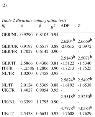
The second step is to test for (bivariate) no-cointegration by means of static cointegration regressions where the null hypothesis of no-cointegration is tested using Augmented Dickey-Fuller (ADF) tests (1979) and the Phillips and Ouliaris (1990) semi-parametrically corrected DF tests (Z). The results are reported in Table 2. Each row corresponds to the ordinary least squares estimation of the static cointegration regression:
(1)
As in the case of the unit root tests, the lag truncation in the case of the ADF and the Z statistics is fixed at four periods. Critical values are taken from Phillips and Ouliaris (1990). In the case of 500 observations and one explanatory variable, they are equal to -2.7619 at 5% and -2.4505 at 10%. The second and third columns are the least squares estimates of the parameters of the static cointegration regression model while the fourth column is the usual R2.
Using this simple framework, we detect a number of significant bivariate cointegrating relationship involving most of the countries, except Italy.
Although extremely simple and appealing for empirical applications, this static regression framework suffers from several drawbacks [see Dolado et al. (1991)], among which we may mention the
impossibility of identifying more than one cointegrated vector among a k-dimensional set of variables with k>2. For this purpose, we follow the approach advocated by Johansen (1988) and Johansen and Juselius (1990). They propose a maximum likelihood approach for both estimating and testing the number of cointegrating relationships in finite order Gaussian VAR models:
(2)
Table 2 Bivariate cointegration tests
ilj R2 ADF Z GER/NL 0.9290 0.8105 0.94 -2.6204b -2.6669b GER/UK 0.9197 0.6517 0.88 -2.0615 -2.0972 GER/FR 1.7027 0.6142 0.90 -2.5140b -2.5071b GER/IT 2.5866 0.4306 0.81 -1.5122 -1.5340 IT/FR -1.2586 1.2806 0.90 -1.7213 -1.7525 NL/FR 1.0200 0.7458 0.93 -2.5874b -2.5497b NL/IT 2.0124 0.5369 0.88 -1.6192 -1.6538 UK/FR 1.4027 0.9054 0.95 -2.5518b -2.5250b UK/NL 0.3399 1.1795 0.90 -3.7778a -4.0583a UK/IT 2.5438 0.6631 0.93 -1.7608 -1.7629
aSignificant at the 5% level. bSignificant at the 10% level.
.which is reparameterised in vector error correction form:
(3)
where εt denotes a k-dimensional normal variate with mean zero and non-singular covariance matrix ∑, and μ is a vector of constant terms. Γi = -I + π1 +...+ πi, with i = 1,. .. , n. It is assumed that the roots of the implicit characteristic polynomial are outside, or at most on the unit circle. The interesting cases arise when rank (Γn) = r<k, in which case there are k — r unit roots in the system (i.e. there are k — r common trends) and r cointegrating relationships. Γn can then be written as αβ', where both α and β are (k x r) matrices of full column rank. The r first rows of β' are the r cointegrating vectors, while the elements of a are the weights of the cointegrating vectors in the different equations. Provided that none of the elements of xt is integrated to an order higher than one, the maximum likelihood estimates of the basis of the cointegrating space is given by the empirical canonical variates of xt_n with respect to ∆xt, corrected for the short-run dynamic and the deterministic components. The number of cointegrating relationships is given by the number of significant canonical correlations. Their significance can be tested by means of a sequence of Likelihood Ratio (LR) tests whose limiting distributing is expressed in terms of vector Brownian motions [see Johansen (1988) and Johansen and Juselius (1990)]. In any empirical application of the Johansen procedure, the lag length in the VAR model has been shown to be important, in terms of both size and power [Boswijk and Franses (1992)]. Using Box-Pierce statistics, it appears that the use of a fourth-order VAR model is sufficient to capture the dynamic present in the data since the resulting residuals display no significant serial correlation. We therefore fit a vector error correction model such as (3) to our five-dimensional vector of variables xt, where the elements of this vector are the stock price series from our selected countries. The model is fitted with a constant in order to capture the trending character of the series.
The results are reported in Table 3. The maximum eigenvalue test does not reject the hypothesis of the presence of a single cointegration vector at the 5% level, while for the trace test, a significant
cointegrating relationship is detected at the 10% level only. This potential cointegrat-ing vector involves all of our five stock prices and, when normalised on the first component, reads as (1.00,
-1.176, 3.443, -3.981, 0.514) with the following ordering of the countries (France, Germany, Netherlands, United Kingdom, Italy). 2
Note that a graphical inspection of the time-series evolution of the linear combination corresponding to the cointegrating vector reinforces the idea that we have isolated a stationary linear combination since the time-series profile of the long-run relationship, represented in Fig. 2, appears as stationary and bounded over time.
Table 3 Johansen's cointegration test
Trace test H0 Max. eigenvalue
1.749 r≤5 1.749 8.459 r≤\ 10.208 12.750 r≤2 22.959 14.766 r≤1 37.7247 32.39'' r = 0 70.1165a Fig, 2.
If we scrutinise this cointegrating vector, it appears that the component corresponding to the Italian stock price is relatively low with regard to the remaining components. A formal LR test for this null hypothesis does enable us to reject it, according to the 5% critical value of a χ2 (1), since the calculated LR test gives a computed value of 3.828. We may thus not reject the hypothesis that Italian stock prices do not share common trends with the remaining stock prices. Once this restriction is imposed, the cointegrating vector reads as (1.00, -0.966, 3.168, -3.173, 0.0). We also note an apparent symmetry in the components. The German and French indices on the one hand, and the UK and Netherlands indices on the other hand, have similar coefficients in the cointegrating vector (with opposite signs). A LR test for this null hypothesis, distributed χ2 (3) under the null, does not enable us to reject this hypothesis (calculated value of 3.870) so that the restricted cointegrating vector finally reads as (1.000, -1.000, 3.047, -3.047, 0.00).
3. Conclusions
Cointegration analysis, which focuses on the analysis of long-run relationships between series, could also be a relevant framework for the study of the potential links between different national stock markets. Using both static regressions and a VAR-based maximum likelihood framework, we find evidence of cointegration between the stock price series of several European countries. This reveals the
existence of some common long-run stochastic trends. An interesting result, which is common to both the static OLS and VAR-based MLE approaches is that, while a long-run relationship seems to hold among European stock prices, Italian stock prices do not seem to influence this long-run relation.
Notes
1These are available from the authors upon request
2 Whether potential ARCH effects or non-normality affect the power is not yet known. We may nevertheless conjecture, in analogy with traditional unit root test - see Urbain (1991), that ARCH and GARCH effects do not imply too important size and power distortions of the cointegration test.
References
Boswijk, H.P. and P.H.B. Franses, 1992, Dynamic specification and cointegration, Oxford Bulletin of Economics and Statistics (forthcoming).
Dickey, D. and W. Fuller, 1979, Distribution of the estimators for autoregressive time series with a unit root, Journal of the American Statistical Association 84, 427-431.
Dolado J., T. Jenkinson and S. Sosvilla-Rivero, 1991, Cointegration and unit roots, Journal of Economic Surveys 4, 249-273.
Fuller, W.A. 1976, Introduction to statistical time series (Wiley, New York).
Johansen, S. 1988, Statistical analysis of cointegration vectors, Journal of Economic Dynamics and Control 12, 231-254.
Johansen, S. and K. Juselius, 1990, Maximum likelihood estimation and inference on cointegration -with applications to the demand for money, Oxford Bulletin of Economics and Statistics 52, 169-210. Newey, W.K. and K.D. West, 1987, A simple positive definite, heteroskedasticity and autocorelation consistent covariances matrix, Econometrica 55, 703-708.
Phillips, P.C.B. and P. Perron, 1988, Testing for a unit root in time series regression, Biometrika 75, 335-346.
Phillips, P.C.B. and S. Ouliaris, 1990, Asymptotic properties of residual based tests for cointegration, Econometrica 58, 165-193.
Solnik, B, 1991, International investments (Addison Wesley, New York). Urbain, J.P., 1991, The behaviour of some unit root tests in the presence of conditional heteroskedasticity, CREDEL Research Paper 9104, University of Liège.