D
D
e
e
v
v
e
e
l
l
o
o
p
p
m
m
R
R
i
i
v
v
e
e
r
r
B
B
i
i
o
o
a
a
s
s
se
s
Isabelle Lavoie, Stéphane Campeau and Claude Fortin
Jennifer Winter, Michelle Palmer
m
m
e
e
n
n
t
t
o
o
f
f
a
a
D
D
i
i
a
a
t
t
o
o
m
m
I
I
n
n
d
d
e
e
x
x
se
e
s
s
s
s
m
m
e
e
n
n
t
t
f
f
o
o
r
r
U
U
s
s
e
e
i
i
n
n
O
O
n
n
Rapport INRS R1270
Isabelle Lavoie, Stéphane Campeau and Claude Fortin
with the collaboration of
Michelle Palmer, Natasa Zugic Drakulic, and Marianne Douglas
x
x
f
f
o
o
r
r
n
n
t
t
a
a
r
r
i
i
o
o
Isabelle Lavoie, Stéphane Campeau and Claude Fortin
Isabelle Lavoie
1Stéphane Campeau
2Claude Fortin
1Michelle Palmer
3Jennifer Winter
3Natasa Zugic Drakulic
4Marianne Douglas
51
Institut national de la recherche scientifique, Centre Eau Terre Environnement, 490 de la Couronne, Québec, Québec, Canada, G1K 9A9
2
Université du Québec à Trois-Rivières, 3351 boul. des Forges, Trois-Rivières, Québec, Canada, G9A 5H7
3
Environmental Monitoring and Reporting Branch, Ontario Ministry of the Environment, 125 Resources Road, Toronto, Ontario, Canada, M9P 3V6
4
Faculty of Environmental Protection, EDUCONS University, Vojvode Putnika, 21208 Sremska Kamenica, Serbia
5
Canadian Circumpolar Institute, Department of Earth and Atmospheric Sciences, University of Alberta, 116 St. and 85 Ave., Edmonton, Alberta, Canada
P
P
r
r
e
e
a
a
m
m
b
b
l
l
e
e
This report has been prepared by Isabelle Lavoie1, Stéphane Campeau2 and Claude Fortin1, with the collaboration of Jennifer Winter3, Michelle Palmer3, Natasa Zugic Drakulic4, and Marianne Douglas5. In it you will find general information on diatom-based monitoring and on the development of version 3.0 of the Eastern Canadian Diatom Index (IDEC: Indice Diatomées de l’Est du Canada) that is, in particular, better adapted for use in Ontario. This new and improved version of the IDEC is the result of a partnership between the Institut national de la recherche scientifique Centre Eau Terre Environnement (INRS-ETE) and the Ontario Ministry of the Environment. The Université du Québec à Trois-Rivières (UQTR) has also actively participated in the development of the IDEC3.0.
As this monitoring tool gains popularity in Québec and Ontario, it is essential to provide upgraded versions of the model. This IDEC3.0 is, therefore, undoubtedly not the last and final version of the index; this monitoring tool is a perpetual work in progress! Over the 10 years of development, improvement and expansion of this biomonitoring tool, there have been multiple people involved to differing extents and several important collaborations with different organisations. Among those who have been involved extensively in this process is Martine Grenier, who played a major role in the development of previous versions of the index. Many of the other author names on the publications and reports have been due to data or funding collaborations with other organisations. However, Isabelle Lavoie and Stéphane Campeau are the core researchers involved in the development of the present version of the IDEC and will remain actively involved in future index development. Indeed, the Watershed Research Laboratory at UQTR (Stéphane Campeau) is in charge of the maintenance of the IDEC database containing more than 1500 diatom samples (as of spring 2012).
The purpose of this document is to provide an overview of the IDEC and its applicability for monitoring urban and agricultural pollution in Eastern Canadian streams (particularly in Québec and Ontario). Fine details about the statistical and modeling techniques will not be presented or discussed in this report. Readers interested in learning more about the development of the IDEC should refer to previous scientific publications related to the index (LAVOIE ET AL., 2006, 2010; GRENIER ET AL., 2006, 2010a). This report is
intended to address the general public concerned with stream biomonitoring and water quality. A detailed manuscript of this new version of the IDEC will be submitted to a special issue of The Science of the Total Environment: “New developments and applications in the use of algae for monitoring rivers”.
W
W
h
h
a
a
t
t
i
i
s
s
t
t
h
h
e
e
i
i
n
n
t
t
e
e
r
r
e
e
s
s
t
t
f
f
o
o
r
r
d
d
i
i
a
a
t
t
o
o
m
m
-
-
b
b
a
a
s
s
e
e
d
d
b
b
i
i
o
o
m
m
o
o
n
n
i
i
t
t
o
o
r
r
i
i
n
n
g
g
?
?
Water chemistry measurements generally used in aquatic ecosystem monitoring are precise and accurate, but do not provide a temporally integrated picture of the response of ecosystems to external stresses, nor do they provide information about the effects of these changes on biological communities. For example, (1) nutrient concentrations do not necessarily reflect the quantity that is bioavailable, (2) high growth rates may deplete ambient nutrient concentrations, resulting in a low concentration of nutrients remaining in the water column at the time of sampling, and (3) traditional analysis of nutrient concentrations interprets the impact of increased concentrations based primarily on the magnitude of the change in nitrogen or phosphorus concentrations without accounting for whether the pre-impact concentration was high or low. In contrast, biological indicators reflect the fact that a shift in nutrients in an oligotrophic system has a different impact on the biota than a shift in nutrients in an eutrophic system.
Biological assessment of water quality can be made using algae, macrophytes, invertebrates or fish as indicators. These organisms respond differently to changes in the chemical and physical environment within different periods of time. Several characteristics qualify algae as excellent bioindicators of water quality: (1) algae are the base of the food chain and are among the first organisms to respond to environmental changes (LOWE &LALIBERTE 1996), (2) algae are very rich in species compared to other organisms, and each species posses specific environmental preferences and tolerances (LOWE & LALIBERTE 1996), (3) algae have short life cycles and respond quickly to environmental variations (MCCORMICK & STEVENSON 1998), and (4) most species are widely distributed among ecosystems and geographic areas (MCCORMICK & CAIRNS
1994).
Diatoms (Bacillariophyceae) are unicellular (eukaryotic) microscopic algae ranging in size from a few to more than 500 microns. Diatoms have a characteristic external skeleton (frustule) made of silica (SiO2), inside of which the cellular content is found
(nucleus, chloroplasts, mitochondria, vacuoles, etc.). Diatoms are particularly abundant in oceans, but are also found in lakes, ponds, streams and rivers, as well as in wetlands and other humid environments. There are two main groups of diatoms: planktonic and periphytic. Planktonic diatoms live in suspension in the water column, while periphytic diatoms are attached to a substrate. Periphytic (or benthic) diatoms constitute an important portion of the biofilm accumulated on rocks or other substrate surfaces.
Diatoms are generally preferred for species-level taxonomy and index development for numerous reasons. First, diatoms are more easily identified to the species level than other algal groups, and the extensive literature on diatom taxonomy offers good-quality pictures. Second, diatom samples are quickly and easily mounted onto permanent slides. Third, diatom community analysis is usually based on counts of a fixed number of diatom valves since individual cells are clearly distinct, compared with filamentous taxa or aggregates of small cell cyanobacteria that are difficult to enumerate as individuals.
Figure 1. Pictures of diatoms showing the various shapes, sizes, and ornamentations.
W
hat is the Eastern Canadian Diatom Index (IDEC)?
The IDEC (LAVOIE ET AL., 2006; 2010) is a diatom-based index that integrates the effects of multiple stressors on streams, most particularly related to eutrophication in agricultural and urban areas. The IDEC scores provide information related to the “distance” from the non-impacted state. The particularity of this biomonitoring tool is the fact that it is a “chemistry-free” index; the position of the sites along the general pollution gradient is strictly determined by diatom community structure and is therefore independent of measured environmental variables. The approach used to develop the IDEC is, in this respect, very different than most diatom-based indices because index values are not derived from a priori established optima and tolerances. The index value indicates the distance, on a scale of 0 to 100, of each diatom community from its specific reference community. A high index value represents a non- or less-impacted site while a low index value represents a more heavily impacted site.
0.01 mm
The siliceous skeleton (frustule) is composedof two valves that fit together analogous to a Petri dish. Each species of diatom has distinct ornaments on the frustule (striae, fibulae, punctae, spines, etc.) allowing for the identification of the species.
0.01 mm
0.005 mm
valvesSince its creation in 2006, the IDEC has been used to evaluate the biological integrity of more than 1500 diatom assemblages collected in more than 700 Eastern Canadian streams (mostly in Québec and Ontario, but also in the Maritimes).
Two upgraded versions have been developed since the publication of the IDEC1.0 (LAVOIE ET AL.,2006), with the newer versions featuring a larger geographic area as well as redefined biological integrity classes that provide a more relevant interpretation of diatom community changes along a pollution gradient (LAVOIE ET AL., 2010; GRENIER ET AL., 2010a). The IDEC is gaining popularity in Québec and has been successfully used to evaluate biological status by various water agencies and by the Québec Ministry of the Environment. We have also calculated IDEC values for Environment Canada as well as for various projects carried out in Canadian universities.
H
ow was the IDEC developed?
In this section we intend to summarize the sampling and analysis procedures, the general approach used to develop the IDEC, as well as the modeling techniques used. You will find illustrations and examples provided here to facilitate the comprehension of certain analyses essential to the modeling of the IDEC. We judged these explanations to be fundamental to the understanding of the new IDEC3.0, which is presented later in this document.
Sampling for diatoms
Benthic diatom assemblages used to assess water quality with the IDEC are collected by scraping the top surface of rocks using a toothbrush. One composite sample per site is collected from riffles where possible. The collected biofilm is preserved with Lugol’s iodine and stored at 4 ̊ C until the samples are processed. Because the biofilm is composed of other groups of algae as well as bacteria, fungi, and small invertebrates, the samples have to be cleaned before diatom identification. Moreover, the cellular content of diatoms also needs to be digested in order to be able to see the details on the frustules. Strong acids or 30% hydrogen peroxide are usually used for diatom sample preparation. Once the samples are digested and only contain diatom frustules, diatom assemblages are mounted onto microscope slides using Naphrax or another mounting medium such as Zrax. Diatom sampling and slide preparation are described in detail in
GONCALVES ET AL. (2011).
Diatom identification
Under a microscope and at 1000x magnification, a minimum of 400 valves per slide are counted and identified to species level where possible. There are numerous taxonomic books to assist with diatom identification, and among the most commonly used are KRAMMER AND LANGE-BERTALOT (1986, 1988, 1991a, 1991b), KRAMMER (2000, 2002, 2003) and LANGE-BERTALOT (2001). During the development of the first version of the IDEC (starting in 2002), we created a user-friendly diatom guide including more than 500 taxa that were observed in our samples from eastern Canadian streams and rivers (LAVOIE ET AL., 2008a). This book is now the main reference used in Québec for diatom analysis and IDEC value calculation.
Diatom assemblage dataset
Although more than 500 taxa were observed in the samples collected in Québec, Ontario and the Maritimes from 2002 to 2011, the diatom database was simplified following the recommendation of LAVOIE ET AL. (2009). Briefly, a taxon is included in the taxa list if it is present with a relative abundance of ≥ 2% in at least one sample. However, many genera are represented by only a few rare species (e,g., species of the genera Pinnularia, Neidium, Stauroneis). After applying the 2% cut-off criteria, these species do not make it to the IDEC taxa list. Although rare, these taxa may be important, and we decided to group them under their respective genera. The number of valves counted for each taxon in each sample is expressed as relative abundance.
Water chemistry dataset
Although the IDEC model was developed solely based on diatom assemblages, water chemistry data were still necessary to assess the direction of the main pollution gradient, and these data were helpful for interpretation in certain circumstances. Water analyses for the majority of sites in Québec and Ontario were performed by the Québec Ministry of the Environment (MDDEP) and the Ontario Ministry of the Environment (MOE) as part of their water quality monitoring programs. Additional sites were selected in Québec and Ontario, and water analyses were performed at the Institut national de la recherche scientifique (INRS) and Trent University. Because diatoms integrate stream water chemistry through time, seasonal averages were used in statistical analyses in order to have a more accurate estimate of the water chemistry conditions characterizing the diatom sampling period (summer). Seasonal averages explain more variance in diatom community structure than one-time chemistry measurements and two month averages because of the variability associated with point measurements (LAVOIE ET AL., 2008b). Average values for the chemical parameters were calculated based on 2 to 6 measurements depending on the availability of data.
Accounting for natural variability
The keystone of the IDEC is its ability to account for the presence of natural variability (mainly due to geology) related to the large geographic area covered by the model. The first step was, therefore, to assess the number of distinct “natural environments” observed across Eastern Canada. This procedure is very similar to the approach used in France where five main hydro-ecoregions were identified (TISON ET AL.,2005,2007). To compensate for natural variability between geographic areas (mainly represented by water pH and conductivity), reference conditions were identified based on diatom communities following the procedure described in GRENIER ET AL. (2006, 2010a). Briefly,
a classification based on a self-organizing map (SOM) was conducted including all the diatom assemblages available. The SOM classification was performed exclusively on biological data, and resulted in a series of “biotypes,” which are groups of samples with similar diatom assemblages.
Figure 2. Illustration of a Self-Organizing Map (SOM)
The samples are then represented on a canonical correspondence analysis (CCA) biplot by coding each assemblage according to its attributed “biotype” established with the SOM. This graphical representation is conducted to determine the reference diatom “biotypes,” and to explore the direction of the alteration gradient. The “biotypes” positioned at the higher end of the alteration gradient on the CCA are indicative of assemblages that represent degraded conditions and are excluded. CCAs are performed with the remaining sites until pH is the only variable associated with the first CCA axis, and the environmental variables associated with stream degradation (for example phosphorus, nitrogen and conductivity) become correlated with the second axis (explaining less variance in assemblage distribution). These consecutive CCAs, gradually excluding diatom biotypes that represent altered conditions, are performed to achieve a final ordination where “biotypes” are distributed principally based on natural pH variability (on the first CCA axis) rather than anthropogenic nutrient enrichment. Once pH becomes the primary gradient structuring the ordination, the “biotypes” that remain in the ordination are selected as reference assemblages. A sub-index is created for each “type” of reference community (LAVOIE ET AL., 2006, 2010).
Self-Organizing Maps (SOMs) belong to the family of Artificial Neural Networks that was developed based on research on artificial intelligence. The SOM allows for a classification of samples based on biotic or abiotic data. For the IDEC, the samples were classified strictly from the diatom assemblages. The samples composed of similar assemblages will occupy cells (hexagones) that are in close proximity, while samples composed of dissimilar assemblages will occupy cells that are far apart. This classification results in the formation of groups of “biotypes” characterized by similar diatom assemblages (this illustration shows five biotypes).
A Canonical Correspondence Analysis (CCA) is an ordination technique that orders samples with similar biological assemblages and abiotic characteristics. The number of axes on a CCA equals the number of abiotic (or environmental) variables included in the ordination. However, the first two axes are the most significant because they summarize most of the variance in the sample distribution. In other words, a CCA provides a means of displaying a large dataset in a two-dimension plot. Similar samples (in terms of biotic and abiotic characteristics) are near each other and dissimilar samples are farther from each other.
Figure 3. Illustration summarizing the steps conducted in the identification of the various “types” of reference assemblages. In this example, there are two “types” of reference assemblages that are found in ecosystems characterized by different water pH under natural conditions.
TN TP pH CON axis 1 a x is 2
Step 1: Each diatom assemblage is represented on a canonical correspondence analysis (CCA) biplot and color coded according to its attributed biotype (derived from the SOM). Total phosphorus (TP), Total nitrogen (TN), conductivity (CON) and pH are closely related to the first CCA axis, suggesting a strong degradation gradient. The biotypes positioned at the higher end of the alteration gradient on the CCA are indicative of assemblages representing degraded conditions. TN TP pH CON axis 1 a x is 2
Step 2: A second CCA is conducted by
excluding the samples (biotypes) that clearly represent degraded conditions. TP and TN are not as strongly associated with the first CCA axis, but this ordination shows that diatom assemblages are still structured by the nutrient gradient. The pH gradient is highly correlated with the first axis. This procedure is repeated until pH is the only variable associated with the first CCA axis, and the environmental variables associated with stream degradation (TP, TN and CON) become correlated with the second axis.
Step 3: The final ordination shows biotypes
that are distributed mainly based on natural pH variability rather than anthropogenic nutrient enrichment. Once pH is the primary gradient structuring the ordination, the biotypes that remain in the ordination are selected as reference communities. In this illustration, there are two different biotypes representing reference (or minimally impacted) conditions. The assemblages coded in red belong to the reference biotype found in naturally higher water pH, while the assemblages coded in yellow belong to the reference biotypes found in naturally more acidic waters. TN TP pH CON axis 1 a x is 2
The remaining diatom assemblages that have not been identified as reference also have to be attributed with a sub-index. This procedure can be tricky in certain circumstances because it relies mostly on the local geological characteristics that are not always available in a data set or that are sometimes ambiguous due to heterogeneity. Different approaches have been used over the years of IDEC development, and more information can be found in previous publications (LAVOIE ET AL., 2006, 2010; GRENIER ET AL., 2006, 2010a).
IDEC: the model
To account for the natural variability that is mainly attributed to the geological characteristics of the various regions sampled, the IDEC is composed of sub-indices reflecting the different “types” of reference diatom assemblages (established based on the SOM and the CCA). This procedure allows discrimination, for example, between the reference diatom assemblages associated with circumneutral/acidic streams located on the Canadian Shield and the communities that represent least-impacted conditions found in agricultural streams of the St. Lawrence Lowlands, which have naturally higher water pH. The distinction between the sub-indices is fundamental to ensure that each stream has the potential to reach a high IDEC value following a hypothetical complete restoration of its ecosystem.
The sub-indices composing the IDEC are developed based on correspondence analyses (CAs), which belong to the family of ordination techniques. A CA is very similar to a CCA, but is conducted based solely on biological data and does not include water chemistry information. This approach is used to obtain a gradual distribution of samples along the first two axes of the ordination. Because most of the variance in the ordination of diatom assemblages is attributed to the first CA axis, we used the score (x-coordinate) of each sample as the index value. In other words, the index value for each site along the gradient of maximum variance is interpreted from its position on the first axis. The position of each site along the gradient of pollution (x-coordinate) is then rescaled to range between 0 and 100 (for practical purposes). A high index value represents a non- or less-impacted site while a low index value represents a more heavily impacted site. The CA-based index does not include any water chemistry data. However, we know from independently conducted CCA that the main variables (correlated with the first axis) structuring the diatoms assemblages are related to agricultural and urban pollution (mainly nutrients and conductivity related to human activities).It is important to note that the CCA ordinations are conducted with the single purpose of interpreting the major gradients structuring diatom assemblages and that the IDEC is strictly determined according to the position of the samples on CA ordinations. The rationale for not using a CCA to determine the IDEC scores is because the position of the samples along the first axis of this type of ordination is influenced by both the diatom assemblages and the water chemistry variables. The main interest for using biota in aquatic ecosystem monitoring is to provide information that is complementary to and not redundant with environmental data such as water chemistry data. The most logical approach, therefore, is to derive bioindication directly from biological assemblages.
Figure 4. Illustration of the CA-based model used to develop each sub-index.
Biological integrity classes
To facilitate the interpretation of the biological “distance” of a site from its reference status (the IDEC score), the alteration gradient was divided into classes reflecting the levels of biological integrity. These classes provide an overall picture of the ecosystem status and are particularly interesting for water quality managers interacting with the general public. In the first version of the IDEC, the classes were arbitrarily defined by dividing the 0-100 gradient into five equal portions. We later modified the method to provide biologically meaningful class boundaries.
We classified diatom communities based on a SOM and obtained “biotypes” for each sub-index. Note that this SOM is different than the SOM used to establish the reference diatom assemblages. Indeed, the SOM realized at this stage includes all diatom assemblages composing the model for a sub-index. This procedure allows for the identification of the different “biotypes” belonging to each sub-index. These biotypes were then used to establish the boundaries between biological integrity classes, as described by GRENIER ET AL. (2010a). Each “biotype” defined by the SOM included multiple samples with similar diatom assemblages. Although similar in terms of diatom communities, the samples included in each biotype showed IDEC values ranging over a portion of the pollution gradient. The density distribution of IDEC values was plotted separately for each of the “biotypes” with a normal curve superimposed.
CA
0
Pollution gradient 0 100 TP TN pH CON TEMP TUR DOCCCA
Correspondence Analysis (CA) is used to determine the position of each diatom assemblage on the main pollution gradient. The position of the samples along the first CA axis represents the IDEC score, rescaled to range between 0 and 100. The CCA including environmental variables was conducted independently to confirm that the first axis is strongly correlated with variables reflecting agricultural and urban pollution. CA axis 1 C A a x is 2
Figure 5. Illustration of the density distribution of the IDEC-values belonging to each “biotype”.
Density distributions and normal curves for all “biotypes” within one sub-index were overlaid on a single plot to provide a continuum of “biotypes” along the alteration gradient. The limits between ecological classes were determined by using the intersection between the normal curve distributions of IDEC values of two adjacent “biotypes”. 0 20 40 60 80 100 0 5 10 15 20 25 0 20 40 60 80 100 0 5 10 15 20 25 0 20 40 60 80 100 0 5 10 15 20 25 0 20 40 60 80 100 0 5 10 15 20 25
IDEC values
N
u
m
b
e
r
o
f
s
a
m
p
le
s
A
B
C
D
For each sub-index, a SOM that includes all diatom assemblages is created.
The SOM resulted in four main “biotypes” labelled A-B-C-D, and IDEC values
are plotted on an histogram with a superimposed normal distribution curve.
Figure 6. Illustration of the approach used to determine the class boundaries.
H
H
o
o
w
w
a
a
r
r
e
e
I
I
D
D
E
E
C
C
v
v
a
a
l
l
u
u
e
e
s
s
c
c
a
a
l
l
c
c
u
u
l
l
a
a
t
t
e
e
d
d
f
f
o
o
r
r
n
n
e
e
w
w
s
s
a
a
m
m
p
p
l
l
e
e
s
s
?
?
The CA-based model can be used to determine the index value for new samples using the formula:
∑
∑
−=
k k ik k k ik k iy
w
u
y
w
x
* * 1 *λ
αThe values for all parameters are derived from the CA model. The sample score for a new diatom assemblage can be rapidly computed based on species abundances. This score is then rescaled to obtain an IDEC value ranging from 0 to 100. A macro in Excel allows for a quick calculation of the IDEC value for a new sample; only the species abundances are required.
Before calculating an IDEC value, it is essential to choose the appropriate sub-index as a function of the natural characteristics of the region sampled. This is by far the most critical step! The choice is sometimes straightforward, but it can be ambiguous in certain regions. Maps were provided to help in the selection of the appropriate sub-index to use in Québec for the previous version of the IDEC (GRENIER ET AL., 2010) and new maps
were created for Québec and Ontario during the development of this new version of the index (see section: Choosing the appropriate sub-index: a few guidelines).
0 20 40 60 80 100 0 5 10 15 20 25
A
B
C
D
IDEC values
N u m b e r o f s a m p le sBiological integrity classes for a sub-index. Each letter corresponds to a “biotype” and the class boundaries are established by the intersection between two adjacent classes.
Biological
IDEC
status
value
Reference
A
state
]70-100]
Slightly
B
polluted
]50-70]
Polluted
C
]20-50]
Highly
D
polluted
[0-20 ]
xi* = sample score on the first CA axis
λ = first axis eigenvalue
α = refers to the scaling method
W*k = species weights
uk = species scores on the first CA axis
W
W
h
h
a
a
t
t
i
i
s
s
n
n
e
e
w
w
w
w
i
i
t
t
h
h
t
t
Additional sampling sites
This new and improved version of the index is the result of a partnership with the Ontario Ministry of the Environment. As a result, a total of 104 new diatom assemblages collected at various sites
database. Numerous additional samples collected in Québec were also included in this new version of the index. As of spring 2012, our overall diatom database contained a total of more than 1500 diatom samples. However, numerous sites
multiple years, and we judged it more appropriate to include only one diatom community per site for the development of the model. This is a novel feature of the IDEC3.0 since the previous versions included samples collected on two consecut
site. Another change to the present version of the IDEC is the exclusion of the diatom communities from the Maritimes that were included in the IDEC version 2.0. This decision was due to the low
because the samples were collected in June rather than in the late summer as for the other samples. Although we did not include the 14 sites from the Maritimes in the model development, the IDEC3.0 should be applicable to this geographical are
geology is comparable to what was observed in Québec and Ontario. database included 648 diatom assemblages
collected at 648 sites between 2002 and 2011.
Figure 6. Distribution of the
across the provinces of Québec and Ontario (2002
t
t
h
h
i
i
s
s
n
n
e
e
w
w
v
v
e
e
r
r
s
s
i
i
o
o
n
n
o
o
f
f
t
t
h
h
e
e
I
I
D
D
E
E
C
C
?
?
sampling sites
This new and improved version of the index is the result of a partnership with the Ontario Ministry of the Environment. As a result, a total of 104 new diatom assemblages distributed across southern Ontario were added to the Numerous additional samples collected in Québec were also included in this As of spring 2012, our overall diatom database contained a total of more than 1500 diatom samples. However, numerous sites were sampled multiple years, and we judged it more appropriate to include only one diatom community per site for the development of the model. This is a novel feature of the IDEC3.0 since the previous versions included samples collected on two consecutive years at the same site. Another change to the present version of the IDEC is the exclusion of the diatom communities from the Maritimes that were included in the IDEC version 2.0. This
low number of samples collected in these pr
because the samples were collected in June rather than in the late summer as for the other samples. Although we did not include the 14 sites from the Maritimes in the model development, the IDEC3.0 should be applicable to this geographical area because the geology is comparable to what was observed in Québec and Ontario. The final
648 diatom assemblages (expressed as relative abundances) sites between 2002 and 2011.
Distribution of the sites visited for the collection of diatom assemblages bec and Ontario (2002-2011).
This new and improved version of the index is the result of a partnership with the Ontario Ministry of the Environment. As a result, a total of 104 new diatom assemblages ario were added to the Numerous additional samples collected in Québec were also included in this As of spring 2012, our overall diatom database contained a were sampled in multiple years, and we judged it more appropriate to include only one diatom community per site for the development of the model. This is a novel feature of the IDEC3.0 since ive years at the same site. Another change to the present version of the IDEC is the exclusion of the diatom communities from the Maritimes that were included in the IDEC version 2.0. This ovinces, and because the samples were collected in June rather than in the late summer as for the other samples. Although we did not include the 14 sites from the Maritimes in the model a because the he final IDEC3.0 (expressed as relative abundances)
The sampling sites were distributed among five ecoregions across Québec and Ontario: Canadian Shield, St. Lawrence Lowlands, Appalachians, Manitoulin-Lake Simcoe, and Lake Erie Lowlands. Although these regions differ in terms of various physico-chemical aspects, geological characteristics are the strongest differentiating factors (Table 1). Table 1. Geology, surficial deposits and land use information for the study area
Ecoregion
Description
St. Lawrence Lowlands
Low-lying region with Paleozoic carbonate bedrock overlain by glacial sediments and post-glacial marine clays, and characterized by fertile soils. Intensive farmlands, large industrial centers, and most of Québec's population.
Canadian Shield
Underlain by igneous and metamorphic rocks such as granite and gneiss (non-carbonate rocks with low buffering capacity) covered by non-calcareous glacial tills (Vincent 1989). Intricate hydrological network of lakes, peat bogs, marshes, beaver ponds, rivers and streams.
Appalachians Sedimentary rocks covered by glacial tills. Moderately impacted by farming
activities. Some areas of the Appalachian region exhibit high concentrations of DOC due to the presence of wetlands.
Manitoulin-Lake Simcoe
Underlain by carbonate-rich, Palaeozoic bedrock, and dominated by a wide variety of deep glacial deposits. The most extensive land use in this ecoregion is agriculture. Urban development is also important.
Lake Erie Lowland
Underlain by carbonate-rich, Palaeozoic bedrock, and dominated by a wide variety of deep glacial deposits. Agriculture is the predominant land use, occupying 65% of the ecoregion. Urbanization (residential, commercial, and industrial) is also important.
(Adapted from Environment Canada (2009))
The diatom taxa list
Within these 648 samples, we identified and counted 406 taxa. Although more than 400 taxa were observed in the samples included in the IDEC3.0, the modeling was achieved using a simplified diatom taxa list. As previously mentioned, a taxon was included in the analysis if it was present with a relative abundance of ≥ 2% in at least one sample. Also, some species were grouped under their genera (Pinnularia, Neidium, Stauroneis, and certain Eunotia). Finally, many taxa that were subdivided into various forms for the previous versions of the IDEC were regrouped for the IDEC 3.0. This was the case, for example, for many forms of Fragilaria capucina, Ulnaria ulna, Eolimna minima. The diatom database was therefore simplified to include a mixture of genera, complexes, species, and varieties, resulting in a final matrix of 277 taxa. The reorganized diatom list, used to develop the IDEC3.0, will facilitate taxonomic analyses and ensure more consistent and reliable results. With the use of the IDEC gaining in popularity and the requirement of more analysts to process the large number of samples, we felt that this procedure was essential. It seemed more appropriate to introduce some imprecision rather than inaccuracy.
Water chemistry data
Numerous physical and chemical parameters were analyzed by the Québec and Ontario ministries, as well as by other agencies. However, due to the number of agencies involved in the construction of this multi-source database, the measured water quality parameters were not consistently the same. For example, while reactive soluble phosphorus data were available for numerous stations, other projects only measured total phosphorus. Similarly, not every project provided information on the various forms of nitrogen, and often only total nitrogen data were available. For this reason, the variables in the compiled chemistry data were total phosphorus, total nitrogen, conductivity, and pH. Moreover, water chemistry data were not available for all sites, or only one or two variables were available, resulting in a final complete chemistry dataset for about half of the 648 sites included in the IDEC3.0. Although our dataset had a limited number of data as well as a restricted number of water chemistry parameters, the information on chemistry-based water quality was sufficient to assess the direction of the main agricultural/urban pollution gradient.
Quality assurance / Quality control
Ensuring that diatom identification is consistent among analysts is a major concern. The previous versions of the IDEC only included diatom samples identified and counted by a single person, which provided a very robust and uniform database. Fortunately, the other analysts who processed the more recent samples from Québec were trained in the same laboratory, which reduced the variability in diatom identification and ensured that mistakes were rapidly corrected. The large database of 104 samples collected in Ontario in 2007 was analyzed by a single person from a different laboratory, and required special attention. Every slide was quickly reanalyzed to make sure that the identification of the common taxa (>2%) agreed with the taxa list used for the IDEC. In addition to the 104 slides, we were also provided with numerous pictures taken by the analyst, which facilitated the comparison between the species lists from the two laboratories. For example, we had to recount and split some taxa when the identification used for the IDEC was more detailed than the list provided by the analyst, and we had to group some taxa when the IDEC list was coarser. We had to find and take pictures of the unidentified taxa (sp.) and provide them with a name or a number that was coherent with the IDEC list. Certain taxa that were very common in the IDEC list were not given the same identification, and therefore, we also modified the names of a few taxa (whether they were originally correctly identified or not). The few alterations made to the 104 sample database ensured uniformity with the IDEC list. Of course, we do not claim that our database is free of misidentifications; however, we are confident that the data used in the IDEC3.0 are very consistent and reliable.
T
he new version of the index: IDEC 3.0
Three types of “reference assemblages”, three sub-indices
The first step in modeling the IDEC is to identify the reference diatom assemblages as described previously. A SOM was created using the total diatom dataset of 648 assemblages and resulted in 23 “biotypes”. A CA was then conducted with the same dataset and each of the 648 diatom assemblage was coded with the 23 SOM “biotypes”. In parallel, we also conducted a CCA by adding the available water chemistry data (total phosphorus, total nitrogen, conductivity, pH) to assess the direction of the main gradients. The “biotypes” clearly indicating non-reference conditions were excluded and another run of CA and CCA was conducted. This procedure was repeated until only the “biotypes” representing least-disturbed/reference conditions remained and were distributed mainly along a natural pH gradient. The CA conducted with the assemblages representing least-disturbed and reference conditions showed three distinct groupings along CA axis 1 (mostly reflecting a natural pH gradient, as well as a natural conductivity gradient to a lesser extent). Based on this distribution of reference diatom assemblages along a pH gradient, the IDEC was developed based on three sub-indices: IDEC-Neutral, IDEC-Alkaline and IDEC-Mineralized. Figure 7 shows the distribution of the reference diatom assemblages coded according to the “biotypes” to which they belong. For example, the “biotypes” coded by grey squares and empty right-triangles represent the reference assemblages typically found in streams located on the Canadian Shield where water pH is naturally lower due to the geology, while the empty left-triangles, grey down-triangles, grey up-triangles and empty stars represent the reference assemblages typically found in streams with naturally higher water pH and conductivity. Figure 7 also shows that even if there are three distinct “types” or groups of reference assemblages along the pH gradient, the transition between the different “types” is gradual because there is a certain degree of overlap.
Figure 7. Correspondence Analysis (CA) showing the distribution of the reference diatom assemblages (coded as a function of their SOM group) along the first CA axis, which mainly reflects a natural pH gradient.
Allocating samples to their corresponding reference assemblage
Now that the first step of the development of the IDEC3.0 showed that the dataset contains three main diatom assemblages representing reference conditions, it is essential to assess which samples go into which sub-index. As previously mentioned, choosing the appropriate “reference diatom assemblage” can be tricky in certain regions. For this new version of the index, we mainly used the selection guidelines defined during our previous work (LAVOIE ET AL., 2006, 2010; GRENIER ET AL., 2006, 2010a). The sub-index IDEC-Neutral should be used in watercourses located on the Canadian Shield where the geology is composed of igneous and metamorphic rocks (eg., granite, gneiss) overlain by organic or non-carbonate glacial deposits. The sub-index IDEC-Alkaline should be used in watercourses located in watersheds composed of clay and siliceous sedimentary rocks (eg., schist, sandstone, shale) overlain by glacial, littoral and marine deposits. These geological characteristics are mostly found in the Appalachians and certain portions of the St. Lawrence Lowlands. Finally, the sub-index IDEC-Mineralized should be used in watercourses located in watersheds mostly composed of carbonate-rich rocks (eg., limestone, dolomite). These geological characteristics are found in south-western Québec and Ontario. To these general guidelines, we had to bring certain modifications and precisions to improve the model. This will be discussed in more detail in the section “Choosing the sub-index: a few guidelines”.
IDEC-Neutral, IDEC-Alkaline, IDEC-Mineralized
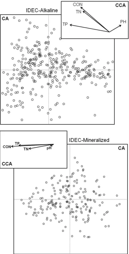
Carefully allocating each non-reference diatom assemblage into the appropriate sub-index resulted in a total of 122, 329, and 197 samples to model the Neutral, IDEC-Alkaline, and IDEC-Mineralize, respectively. The index values correspond to the position of each site along the first CA axis (x-axis) after rescaling the gradient to obtain a value ranging between 0 and 100. The reference assemblages (reference sites) are on the right and the most impacted sites are on the left. The CCA is presented only to show the major gradient structuring the assemblages, but is not involved in the IDEC calculation. The arrows for the pH gradients in each CCA are very short, indicating that this variable does not influence diatom assemblage distributions, and that pollution-related variables (nutrients and conductivity from human activities) are the main driving gradients.
Figure 8a. Correspondence Analysis (CA) used to develop the sub-index IDEC-Neutral. The positions of the samples along the first CA-axis correspond to the IDEC scores (after being rescaled to range between 0 and 100).
Figure 8b. Correspondence Analysis (CA) used to develop the sub-index IDEC-Alkaline. The positions of the samples along the first CA-axis correspond to the IDEC scores (after being rescaled to range between 0 and 100).
Figure 8c. Correspondence Analysis (CA) used to develop the sub-index IDEC-Mineralized. The positions of the samples along the first CA-axis correspond to the IDEC scores (after being rescaled to range between 0 and 100).
General qualitative classes
The classes provide a rapid and easy overall picture of the watercourse biological status within a watershed. Following the method previously described, we classified diatom assemblages within each of the three sub-indices using SOMs. This classification resulted in four distinct “biotypes” for each sub-index.
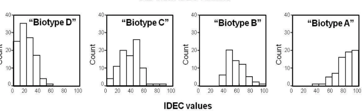
The density distribution of IDEC values was plotted separately for each of the “biotypes” labelled A, B, C, and D. “Biotype A” includes the diatom assemblages representing the best water quality conditions we found, with the highest IDEC values.
Figure 10. Density distribution of IDEC values within each of the four “biotypes”
Figure 9. Self-organizing map (SOM) for the sub-index IDEC-Alkaline showing the four “biotypes” used to establish the general biological integrity classes. The same procedure was used for the IDEC-Neutral and IDEC-Mineralized.
Normal distribution curves were derived from these distributions. The four curves representing the four “biotypes” were then overlaid on one figure. This was repeated for each sub-index. The previous version of the IDEC used the intersection of two adjacent curves to establish the biological class boundaries. Because of the strong overlap between the curves, both in the IDEC2.0 and with the present version, we decided to position the class boundary in the middle of two distribution maxima. Although the overlap between “biotypes” results in class boundaries that are not always clearly distinct, we feel that this approach is much more ecologically meaningful than separating the 0-100 IDEC gradient into 4 or 5 equal classes. These classes are derived from the maximum ecological distance between diatom groups (from the SOM), and the transition from one class to another reflects an important shift in the diatom assemblage structure. The proposed classes based on “biotypes” provide a more relevant interpretation of the structural changes along the degradation gradient.
Figure 12. Normal curves derived from the density distribution of IDEC values for each “biotype.” The class boundaries represent the mid-point between the maxima of two adjacent curves.
IDEC-Neutral
IDEC-Alkaline
Figure 13. Biological integrity classes for each sub-index and their corresponding ranges in IDEC values.
Biological status of Ontario streams and rivers
The development of the IDEC model allowed us to evaluate the position of numerous sties sampled in Ontario along the general pollution gradient. Figure 14 shows the distribution of the sites sampled in Ontario as well as their biological integrity classes. The IDEC values are presented in Appendix 1. Table 2 presents examples of the best and the worst sampling stations in Ontario for each sub-index. Briefly, most of the small creeks and streams sampled on the Canadian Shield in Ontario showed excellent biological integrity. It is interesting to note that for one golf course, the IDEC classes dropped from A to D depending on the sampling station (small creeks sampled on and near the Grandview golf course). Diatom assemblages showed a clear shift that was most likely due to nutrient input from fertilizers, and this shift in index values for sites in relatively close proximity underscores the sensitivity of the IDEC. It is not surprising to observe that the watercourses sampled in Toronto showed relatively poor water quality, as the high proportions of impervious areas would be expected to increase urban runoff. Numerous water bodies had a good biological status in the upstream portion and a lower IDEC value in the downstream portion. This was the case, for example, for certain stations in the Grand River watershed.
IDEC-Neutal IDEC-Alkaline IDEC-Mineralized Biological IDEC status value Reference A state [70-100] Slightly B polluted [45-70[ Polluted [20-45[ C Highly D polluted [0-20[ Biological IDEC status value Reference A state [70-100] Slightly B polluted [45-70[ Polluted [25-45[ C Highly D polluted [0-25[ Biological IDEC status value Reference A state [75-100] Slightly B polluted [45-75[ Polluted [25-45[ C Highly D polluted [0-25[
Figure 14. Map of Ontario with biological status of streams To ro n to K in g st o n O tt a w a C o rn w a ll W in d so r L a k e O n t a r io L a k e E r ie L a k e H u ro n H u n ts v il le
A
B
C
D
Table 2. Examples of sampling stations in Ontario for each sub-index that had high and low IDEC values.
Sampling station IDEC
value
Biological status IDEC-Neutral
Small tributary to Harp Lake near Huntsville 90 A
Small tributary to Harp Lake near Huntsville 78 A
Small tributary on Grandview golf course near Huntsville 100 A
Small tributary on Grandview golf course near Huntsville 4 D
Stoney Creek 16 D
IDEC-Alkaline
North River 95 A
Fall River 77 A
Black River 71 A
Gananoque River (downstream) 21 D
IDEC-Mineralized
Coldwater River (near Midland) 100 A
Ouse River 100 A
Moira River 96 A
Speed River (upstream) 100 A
Wye River (upstream near Midland) 83 A
Etobicoke Creek 0 D
Mimico Creek 0 D
South Thames River 7 D
Don River 12 D
Choosing the appropriate sub-index: a few guidelines
For people interested in using the IDEC to monitor the biological integrity of new sites, the first and most important step is to select the appropriate sub-index. Since geological characteristics of the watershed are among the most important criteria for the distinction between sub-indices, it is not surprising that most sampling sites can be allocated into the appropriate sub-index based on their ecoregion (Canadian Shield, St. Lawrence Lowlands, Appalachians, Manitoulin-Lake Simcoe, Lake Erie Lowlands).
As a general rule, the IDEC-Neutral is used for sampling sites located on the Canadian Shield in Québec and Ontario, the IDEC-Alkaline is used in the Appalachians and some portions of the St. Lawrence Lowlands, and the IDEC-Mineralized is used in the south-western portion of Québec and the Ontario Lowlands. In the process of remodeling this new version of the IDEC, a few precisions and modifications were added to these
general rules based on the addition of new reference stations and as a result of a thorough examination of Eastern Canadian geology and its influence on pH and conductivity values of watercourses. In light of the revised geological properties of each region covered by the IDEC, a map was created to help in the choice of the appropriate sub-index.
Figure 15. Map showing the sub-index to use for different regions of Ontario and Québec.
The decision regarding the sub-index can also be facilitated by the few selection “rules” presented in the following table (Table 3) created as a function of the dominant geology (> 50% of the area) in the watershed upstream of the sampling station. The IDEC-Neutral is used on the Canadian Shield where the substratum is dominated by felsic rocks such as granite, rhyolite, tonalite and orthogneiss (non-carbonate with low buffering capacity). These watersheds are often overlain by non-calcareous tills, fluvioglacial deposits, and wetlands. The median pH and conductivity values under natural conditions are 7.2 and 40 µS/cm, respectively. In certain cases, the IDEC-Neutral can also be used in the St. Lawrence Lowlands and the Appalachians in small watersheds occupied by wetlands.
Neutral Alkaline Mineralized IDEC3.0 Reference sites Toronto Kingston Ottawa Cornwall Windsor Lake Ontario Lake Erie Lake Huron Huntsville Neutral Alkaline Mineralised Montreal Québec Ottawa
The IDEC-Alkaline should be used in watersheds located on the Canadian Shield where the substratum is dominated by intermediate and mafic rocks such as diorite, gabbro, basalt, anorthosite, and syenite. This sub-index is also appropriate in watersheds dominated by marble formations. The IDEC-Alkaline is used in the Canadian Shield valleys that are overlain by marine and glaciolacustrine clay and limonite. In the St. Lawrence Lowlands and the Appalachians, the IDEC-Alkaline is used in watersheds characterised by a substratum dominated by clay or siliceous sedimentary rocks such as shale, schist, sandstone, and conglomerates. These watersheds are generally overlain by marine and glacial deposits. The median pH and conductivity values under natural conditions are 7.8 and 104 µS/cm, respectively.
The IDEC-Mineralised should be used in watersheds with substratum dominated by carbonate-rich rocks such as limestone and dolomite. These geological formations are found in the Lowlands of the St. Lawrence River and Lake Erie, as well as in the Manitoulin-Lake Simcoe ecoregion in Ontario. These regions are generally overlain by marine and glacial deposits. The median pH and conductivity values under natural conditions are 8.3 and 447 µS/cm, respectively.
The selection of the appropriate sub-index is sometimes difficult when a watershed covers two ecoregions from upstream to downstream. In most cases, the ecoregion located upstream will dictate the choice of the sub-index. In Québec, this situation is often encountered where watersheds spread across the Canadian Shield and the St. Lawrence Lowlands (e.g., Jacques-Cartier River, St. Maurice River). Because a large area of the watershed of these rivers is located on the Canadian Shield, this ecoregion will have a strong influence on the physical and chemical characteristics of the water even in the downstream portion. However, in certain cases, it becomes difficult to make a decision when relatively equal areas of the watershed are spread across two ecoregions, such as for the Moira River in Ontario that is split between the Canadian Shield and the St. Lawrence Lowlands. In these cases, it is difficult to establish where the physical and chemical properties of the river start to reflect new geology because the transition is gradual. Users should be particularly careful in choosing the sub-index in these circumstances (e.g., at the margin of the Canadian Shield in Ontario) and should also be careful in the IDEC value interpretation.
The selection of the appropriate sub-index should be achieved independently for the main watercourse and its tributaries. It is frequently encountered that different sub-indices are used.
Table 3. Guidelines to select the appropriate sub-index to use depending on the region.
IDEC-Neutral IDEC-Alkaline IDEC-Mineralized
Natural pH Median Centiles (20e – 80e) 7.2 6.7 – 7.4 7.8 7.6 – 8.0 8.3 8.0 – 8.5 Natural conductivity Median Centiles (20e – 80e) 40 µS/cm 27 - 58 104 µS/cm 62 - 150 447 µS/cm 379 - 533 Canadian Shield : Southern and Central Laurentians (Québec), Algonquin-Lake Nipissing (Ontario), Lake Temiscamingue Lowlands Felsic rocks (granite, rhyolite, orthogneiss, tonalite, etc.) Covered by non-calcareous glacial tills, fluvioglacial or organic deposits.
Intermediate and mafic rocks (gabbro, basalt, anorthosite, syenite, diorite) Carbonate metasedimentary rocks (marble) Valleys covered by marine or glaciolacustrine clays
and silts in the
Canadian Shield. Never used. St. Lawrence Lowlands and Appalachians Small watersheds covered by wetlands.
Clay and siliceous sedimentary and metasedimentary rocks (mudrocks, siltstones, sandstones, and conglomerates)
Covered by marine clays and silts or glacial deposits.
Limestone and dolostone covered by marine clays and silts.
Lake Erie Lowlands and Manitoulin-Lake Simcoe (Ontario)
Never used. Never used. Limestone and dolostone covered by carbonate-derived tills, glaciolacustrine and glaciofluvial deposits or marine clays.
How can water managers use the IDEC for bioassessment?
The IDEC3.0 is now ready for use in Ontario and is administered by the Ontario Ministry of the Environment. Conservation authorities, provincial and local governments, and other stakeholders may contact the ministry to request IDEC3.0 analysis. For more information, please contact:
Jennifer Winter
Supervisor, Sport Fish and Biomonitoring Unit Environmental Monitoring and Reporting Branch 125 Resources Road, Toronto
Ontario, Canada M9P 3V6
References
GONCALVES C, WINTER J, JARVIE S, JONES C (2011) An Algal Bioassessment Protocol for Use in Ontario Rivers. 49 pages. Ontario Ministry of the Environment Report, PIBS# 8618e.
GRENIER M, CAMPEAU S, LAVOIE I, PARK Y-S, LEK S (2006) Diatom reference
communities and restoration goals for Quebec streams (Canada) based on Kohonen Self-Organizing maps and multivariate statistics. Canadian Journal of Fisheries and Aquatic Sciences 63: 2087–2106.
GRENIER M, LAVOIE I, ROUSSEAU A,CAMPEAU S. (2010a) Defining ecological thresholds to determine class boundaries in a bioassessment tool: the case of the Eastern Canadian Diatom Index (IDEC). Ecological Indicators 10: 980–989.
GRENIER M, LEK S,RODRIGUEZ MA,ROUSSEAU A N, CAMPEAU S (2010b) Algae-based biomonitoring: Predicting diatom reference communities in unpolluted streams using classification trees, random forests, and artificial neural networks. Water Quality Research Journal of Canada 45 : 413–425.
KRAMMER K (2000) The genus Pinnularia. Diatoms of Europe. Diatoms of the European Inland Waters and Comparable Habitats. Vol. 1. 703 pages. In H. Lange-Bertalot, editor. A.R.G. Gantner Verlag KG, Ruggell.
KRAMMER K (2002) Cymbella. Diatoms of Europe. Diatoms of the European Inland Waters and Comparable Habitats. Vol. 3. 584 pages. In H. Lange-Bertalot, editor. A.R.G. Gantner Verlag KG, Ruggell.
KRAMMER K (2003) Cymbopleura, Delicata, Navicymbula, Gomphocymbellopsis, Afrocymbella. Diatoms of Europe. Diatoms of the European Inland Waters and Comparable Habitats. Vol. 4. 530 pages. In H. Lange-Bertalot, editor. A.R.G. Gantner Verlag KG, Ruggell.
KRAMMER K, LANGE-BERTALOT H (1986) Bacillariophyceae. 1. Teil: Naviculaceae. In H. Ettl, J. Gerloff, H. Heyinig, and D. Mollenhauer, editors. 876 pages. Süβwasserflora von Mittleuropa, Band 2/1. Gustav Fischer Verlag, Stuttgart/New York.
KRAMMER K, LANGE-BERTALOT H (1988) Bacillariophyceae. 2. Teil: Bacillariaceae, Epithemiaceae, Surirellaceae. In H. Ettl, J. Gerloff, H. Heyinig, & D. Mollenhauer, editors. 611 pages. Süβwasserflora von Mittleuropa, Band 2/2. Gustav Fischer Verlag, Stuttgart/New York.
KRAMMER K, LANGE-BERTALOT H (1991a) Bacillariophyceae. 3. Teil: Centrales,
Fragilariaceae, Eunotiaceae. In H. Ettl, J. Gerloff, H. Heyinig, & D. Mollenhauer, editors. 596 pages. Süβwasserflora von Mittleuropa, Band 2/3. Gustav Fischer Verlag, Stuttgart/Jena.
KRAMMER K, LANGE-BERTALOT H (1991b) Bacillariophyceae. 4. Teil: Achnanthaceae
H. Heyinig, & D. Mollenhauer, editors. 437 pages. Süβwasserflora von Mittleuropa, Band 2/4. Gustav Fischer Verlag, Stuttgart/New York.
LANGE-BERTALOT,H (2001) Navicula sensu stricto, 10 genera separated from Navicula sensu lato, Frustulia. Diatoms of Europe. Diatoms of the European inland waters and comparable habitats. Vol. 2. 526 pages. In H. Lange-Bertalot, editor. A.R.G. Gantner Verlag KG, Ruggell.
LAVOIE I, GRENIER M, CAMPEAU S, DILLON PJ (2006) A diatom-based index for water quality assessment in eastern Canada: an application of Canonical Analysis. Canadian Journal of Fisheries and Aquatic Sciences 63: 1793–1811.
LAVOIE I,HAMILTON P,CAMPEAU S,GRENIER M, DILLON PJ (2008a) Guide d'identification des diatomées des rivières de l’est du Canada. Presses de l’Université du Québec (PUQ), 230 pages.
LAVOIE I,DARCHAMBEAU F,CABANA G,DILLON PJ,CAMPEAU S (2008b) Are diatoms good integrators of temporal variability in stream water quality? Freshwater Biology 53: 827– 841.
LAVOIE I,DILLON P,CAMPEAU S (2009) The effect of excluding diatom taxa and reducing taxonomic resolution on multivariate analysis and stream bioassessment. Ecological Indicators, 9: 213–225.
LAVOIE I, GRENIER M, CAMPEAU S (2010) The Eastern Canadian Diatom Index (IDEC) Version 2.0: Including meaningful ecological classes and an expanded coverage area that encompasses additional geological characteristics. Water Quality Research Journal of Canada 45: 463–477.
LOWE R L, LALIBERTE G D (1996) Benthic stream algae: distribution and structure. Methods in Stream Ecology. In Stream ecology: field and laboratory exercises. F R Hauer and G A Lamberti, editors. Pages 269–293. Academic Press, San Diego.
MCCORMICK PV,STEVENSON RJ (1998) Periphyton as a tool for ecological assessment and management in the Florida everglades. Journal of Applied Phycology 34:726–733. MCCORMICK PV,CAIRNS J (1994) Algae as indicators of environmental change. Journal of Applied Phycology 6: 509–526.
TISON J, PARK Y S, COSTE M, WASSON J G, ECTOR L, RIMET F, DELMAS F (2005) Typology of diatom communities and the influence of hydroecoregions : A study on the french hydrosystem scale. Water Research 39: 3177–3188.
TISON J, PARK Y S, COSTE M, WASSON J G, ECTOR L, RIMET F, DELMAS F (2007) Predicting diatom reference communities at the french hydrosystem scale: A first step towards the definition of the good ecological status. Ecological Modelling 203: 99–108.