HAL Id: inria-00182078
https://hal.inria.fr/inria-00182078
Submitted on 7 Nov 2007HAL is a multi-disciplinary open access archive for the deposit and dissemination of sci-entific research documents, whether they are pub-lished or not. The documents may come from teaching and research institutions in France or abroad, or from public or private research centers.
L’archive ouverte pluridisciplinaire HAL, est destinée au dépôt et à la diffusion de documents scientifiques de niveau recherche, publiés ou non, émanant des établissements d’enseignement et de recherche français ou étrangers, des laboratoires publics ou privés.
approche statistique
Dizan Alejandro Vasquez Govea
To cite this version:
Dizan Alejandro Vasquez Govea. Estimation de mouvement des obstacles mobiles: une approche statistique. [Travaux universitaires] 2003. �inria-00182078�
G
D
’É
A
S
: I
, V
R
Estimation de Mouvement des Obstacles Mobiles: Un
Approche Statistique
(Motion Estimation for Mobile Obstacles: A Statistical Approach)
Dizan Vasquez
Date de Soutenance: 11 Septembre 2003
Encadrant: Dr. Thierry Fraichard
Projet préparé au sein du projet CYBERMOVE,
au Laboratoire GRAphique, VIsion, Robotique
à Inria Rhône-Alpes
ZIRST, 655 av. de l’Europe
38330 Montbonnot St. Martin
1 Introduction 1
1.1 Problem Overview . . . 1
1.2 Objectives . . . 2
1.3 Contributions . . . 2
1.4 Structure of the Document . . . 3
2 Related Works 4 2.1 Motion and Motion Models . . . 4
2.2 Generative Motion Models . . . 5
2.2.1 Parametrical Models . . . 5 2.2.2 Random Models . . . 6 2.2.3 Intentional Models . . . 6 2.2.4 Estimation . . . 6 2.2.5 Related approaches . . . 7 2.2.6 Analysis . . . 7
2.3 Descriptive Motion Models . . . 8
2.3.1 Grid Models . . . 9
2.3.2 Cluster based Models . . . 11
2.3.3 Other Models . . . 14
2.4 Data Clustering . . . 14
2.4.1 De?nition of the problem . . . 14
2.4.2 Similarity Measures . . . 15 2.4.3 Clustering Techniques . . . 16 2.4.4 Hierarchical Clustering . . . 16 2.4.5 Partitional Clustering . . . 18 2.4.6 Fuzzy Clustering . . . 20 3 Proposed Approach 21 3.1 Learning Motion Patterns . . . 22
3.1.1 Similarity Measure . . . 22
3.1.2 Clustering Algorithm . . . 22
3.1.3 Calculating Class Statistical Parameters . . . 25
3.2 Estimating Trajectories . . . 26
3.2.1 Partial Distance . . . 26
3.2.2 Calculating Likelihood . . . 26
3.2.3 Cluster Probability . . . 26
3.3 Analysis . . . 27
4 Experimental Results 28 4.1 Generation of the Training Set . . . 28
4.2 Estimation of K and clustering . . . 29
4.3 Generation of the Test Set . . . 30
4.4 Benchmarking . . . 31
4.5 Graphical Representation of Estimation . . . 33
4.6 Analysis . . . 33
5 Conclusions 37 5.1 Summary and Contributions . . . 37
2.1 Raw trajectories of people in an oEce environment . . . 9
2.2 Statistical Grid for example data . . . 10
2.3 Resulting Clusters for example data . . . 13
2.4 Clustering Techniques . . . 16
2.5 Example Clusters (taken from [Jain 99]) . . . 17
2.6 Corresponding Dendogram (taken from [Jain 99]) . . . 17
2.7 Distance Between Clusters . . . 18
4.1 The INRIA entry Hall . . . 29
4.2 Examples of generated clusters for the three algorithms. . . 31
4.3 Benchmark Results . . . 32
4.4 Trajectory Estimation for DiJerent Instants . . . 33
4.5 Results by Number of Clusters . . . 34
4.6 Clustering times . . . 35
4.7 The Camera View . . . 36
4.8 Some Clusters obtained using real data . . . 36
4.1 Clustering Results . . . 30
The main objective of this work is to search for a motion estimation technique for vehicles and pedestrians having the following properties:
a) It should produce estimations with a long Time Horizon.
b) It should be as general as possible and work with many diJerent kinds of objects. c) It should be fast enough to give estimations in real time.
We propose a motion estimation technique based on pairwise clustering which.veri?es the required properties.
We have implemented and tested our approach, comparing it with a technique that we consider to represent the state of the art in clustering techniques. In order to perform the comparison, we propose a benchmark that can be used to test other motion estimation techniques.
Keywords: Motion Estimation, Pairwise Clustering, Trajectory Clustering, Tra-jectory Prediction
Introduction
1.1
Problem Overview
In order to survive, most animals and every intelligent being have to be able to navigate purposefully within the environment they inhabit. One of the greatest challenges of navigating in a real environment is to deal with the obstacles populating it. This challenge is further complicated by the fact that many of those obstacles are not static: they are involved in activities and their situation evolves over time. In order to successfully interact with moving obstacles, it is necessary to predict their movements. Motion modeling and estimation is a research area which has applications in many diJerent ?elds, ranging from video surveillance [Koller 94] to robot navigation [Kyriakopoulos 92]. Many techniques have been proposed in the literature, however, most of the existing proposals share an important drawback: the estimations they provide are only sound during a short time interval. We say that these techniques have a short Time Horizon.
If we can ?nd techniques having a longer Time Horizon, we would have more trustful navigation schedules. Hence, it is very important to develop motion models for obstacles that allow to estimate trajectories as far as possible in the future and with a maximum of certainty. This problem, however, sets signi?cant diEculties: a dynamic environment is often populated by many kinds of moving obstacles (cars, pedestrians, industrial robots, etc.) having very diJerent motions resulting from a wide variety of factors (kinematic constraints, dynamic constraints, intentionality, etc.) In order to estimate their motion, it would be necessary to have a model which takes into account the features of each kind of obstacle. The problem with such a model is that it would be utterly complex. The preferred alternative is to have many diJerent models, one for each kind of obstacle, unfortunately, the development of those specialized models implies previous domain knowledge, and its reusability is severely limited due to its
speci?city.
In this context, we would like to have motion estimation techniques having a good compromise between generality and complexity so that they can be applied to a wide spectrum of situations while still having long Time Horizons. We believe in the possi-bility of such a technique, and propose in this document an approach that, we hope, constitutes a step towards it.
1.2
Objectives
This work aims at ?nding a motion estimation technique that can be implemented in an actual project: ParkView. The goal of ParkView is to develop autonomous robot vehicles able to evolve in a parking lot. In order to attain this autonomy, a mechanism is needed that allows to predict motion of obstacles which populate the car’s environment, notably other cars and pedestrians. Given the characteristics of the project, the resulting technique should verify the following properties:
1. It should produce estimations with a long Time Horizon.
2. It should be as general as possible and work with many diJerent kinds of objects. 3. It should be fast enough to give estimations in real time.
1.3
Contributions
As a result of our work we present the following contributions:
• We propose a cluster-based motion estimation technique which veri?es the prop-erties mentioned in section 1.2. With this technique:
— We propose a dissimilarity metric that allows the use of pairwise cluster-ing algorithms. To our knowledge, this is a novel approach to trajectory clustering.
— We propose a way to calculate the number of clusters to be used in the clustering solution.
— We present an algorithm to calculate the mean value of a cluster of trajec-tories and then use this mean value in order to calculate the corresponding standard deviation.
— We propose a way to estimate the likelihood that a partially observed tra-jectory belongs to a given cluster.
• We implemented and tested our approach using simulated data.
• Finally, we compare our results against those of a technique [Bennewitz 02] that we consider as representing the state of the art in this kind of estimators. In order to perform this comparison we propose a benchmark that may be useful for evaluating other techniques.
1.4
Structure of the Document
The introduction explained in a loose way some of the reasons behind the interest on motion estimation. It also de?ned the main goal of our work, as well as three required properties of the resulting technique. Finally, it succinctly describes our contributions. The remainder of this document is organized as follows.
Chapter 2 The second chapter reviews basic notation and concepts which are used throughout the document. A classi?cation of existing motion models in two categories (Descriptive and Generative) is proposed based on the underlying representation. Both categories are brieKy explained and discussed. Finally, given that our approach strongly relies on data clustering, an overview of this domain is given.
Chapter 3 In the third chapter, we explain the details of the approach we propose. We describe the learning stage, which is based on pairwise clustering by means of a measure of dissimilarity between trajectories. We propose a way of estimating the number K of clusters of a clustering instance. We explain how we calculate statistical parameters for each cluster and how we use these values in order to estimate motion. Finally, we discuss the theoretical advantages and drawbacks of our approach.
Chapter 4 In the fourth chapter, we present an overview of the tests we have per-formed. We describe the dataset generation process. After that, we comment the results we obtained using the diJerent clustering algorithms on the dataset. Finally, we explain the benchmarking process and discuss the results we obtained. Chapter 5 The last chapter summarizes the main issues of this work, gives directions to future work and discusses extensions and improvements of the models and algorithms presented.
Related Works
Motion has always intrigued humanity. Zeno’s famous paradoxes testify the fascination exerted by motion in humanity since the ancient times. In all these years, a huge body of work has been developed around the study of moving objects. This chapter will present an overview of the techniques that have been developed in order to model and predict an object’s motion; It will also provide the reader with a general discussion of data clustering, which constitutes the hearth of the approach we propose.
2.1
Motion and Motion Models
Before going any further, it is important to de?ne motion, what it is? To us, and throughout this document, motion is de?ned as the change in position and / or orien-tation of the parts of an object that takes place as time passes.
At any given moment t an object is said to be in a certain con guration, which is a mathematical speci?cation of the position and orientation of the diJerent parts of the object with respect to a ?xed frame. For example, in the case of a single rigid object which is able to move on a plane, a con?guration q is speci?ed using a vector q = [x, y, ]. We call con guration space (represented by the symbol C) the space de?ned by all the possible con?gurations for an object in the absence of obstacles, so that every con?guration is represented by a point in C. In the case of a rigid object on the plane, the con?guration space is 3-dimensional.
In general, there are two ways of modeling motion: The ?rst one, often called descriptive, or phenomenological models, represents a particular motion instance as a succession of con?gurations in a way very similar to a series of photos. Usually, a descriptive model is represented as list of con?gurations q = {q0, q1, ..., qT} where each
qt C represents the con?guration of the object in the instant t and T represents the
total duration of the motion.
The other modeling approach tries to model motion as a function of a given num-ber of parameters, thus, the same model can be used to represent multiple motion instances. A very important factor in this modeling approach is the introduction of time t as a parameter; this allows to model the evolution of dynamic systems and, by changing the value of t, predicting future con?gurations, or estimating con?gurations previous to the ?rst one that was observed. Due to this capability of representing "unseen" con?gurations, these models are called generative. A generative model is a function q(t) of time q : [0, T ] C which outputs the corresponding con?guration q(t) for a given instant t.
The following two sections provide a deeper, but far from exhaustive, description of both modeling approaches.
2.2
Generative Motion Models
Generative motion models are based on physical laws. They work by calculating acceleration ¨q(t) as a function of time and then integrating once to calculate velocity q(t) and twice to get the actual con?guration q(t) the whole process is outlined in the following equations: q(t) = q(0) + T 0 ¨ q( )d (2.1) q(t) = q(0) + T 0 q( )d (2.2)
What distinguishes diJerent Generative Motion Models is the way they de?ne ¨q. In the rest of his section, we de?ne a classi?cation of generative motion models based on [Zhu 90] A particular approach can correspond to just one category or a combination of them.
2.2.1
Parametrical Models
In parametrical models acceleration is considered to follow a known form:
¨
q(t) = p(t) (2.3)
Where p(t) is a function and p is the constant parameter vector for . For example, if p(t) is a ?rst degree polynomial of the form p(t) = c1t + c2 = 0 then
p = [c1, c2] So, if we know the form of and the parameters p, as well as the velocity
con?guration after a given interval T . applying expressions 2.1 and 2.2. An example of a parametrical model is [Kalman 60] where acceleration is supposed to be constant.
2.2.2
Random Models
Random Models assume that changes in acceleration are determined by a given prob-ability distribution, such as Gaussian, Uniform or Poisson.
¨
q(t) = (t) (2.4)
Where (t) is function which generates a vector using a given probability distri-bution. An example can be seen in [Strehl 98] where the probability distribution for ¨q is iteratively calculated and (t) is generated taking the acceleration with maximum probability.
2.2.3
Intentional Models
In intentional models, objects move along a scheduled path, usually attempting to accomplish one or more goals. The obstacle can react to the environment and even perform collision avoidance. For this model, we characterize acceleration as:
¨
q(t) = e(t) (2.5)
Where e(t) is the acceleration chosen by the obstacle’s intentional strategy. We can wonder about the nature of the diJerence between expression 2.4 and 2.5 which have identical form. If we take a closer look, they are very diJerent: (t) is just a vector (depending on nothing but the underlying probability distribution and its parameters), while e(t) is usually a very complex function strongly dependent on the actual con?guration of the world, the internal state of the object and the navigation strategy itself. Moreover, in real life, access to the particular motion strategy (and thus to the form of e) is frequently impossible. And estimation is a very diEcult task even when the motion strategy is known. As a matter of fact, motion planning can be viewed as an example of an intentional model (see [Latombe 91]).
2.2.4
Estimation
Theoretically, if we have an appropriate motion model and if we know the value of all its parameters as well as its actual velocity and con?guration, then future con?guration prediction is straightforward. Unfortunately, in most real-life cases, some or all of those parameters are unknown and have to be estimated. The same applies to velocity and con?guration.
The process of estimation uses a set of observations, gathered through some kind of measuring device or sensor, in order to approximate the values of the unknown variables for the given motion model.
2.2.5
Related approaches
An estimation technique is constituted of a motion model, as well as state and pa-rameter estimation processes. The vast majority of approaches found in literature are based in Physics Laws (uniform accelerated motion) as motion models and some variation of Kalman Filter or Extended Kalman Filter estimation processes.
The Kalman Filter [Kalman 60], is an optimal state estimator. Its origin lies in the problem of estimating satellite and aircraft trajectories using radar data. In this problem, con?guration (x, y, z) and velocity (x, y, z) should be estimated from the observation of two angles: site and azimuth ( , ). Future state prediction can be performed using the estimated values of con?guration and velocity.
A dynamic programming approach to estimation is proposed in [Larson 66], the paper shows that the technique can be reduced to a Kalman Filter. A Kalman Filter improved using Montecarlo Simulation is applied in [Chang 77] to robot navigation.
More recently, recursive formulations of the Extended Kalman Filter have been proposed by [Blostein 95]. A two-layer Extended Kalman Filter is applied to tracking moving targets in [Kawase 98].
Other approaches for state and parameter estimation for generative models have been used. The application of fuzzy logic and neural networks to state estimation is studied in [Patt 98]. Local avoidance using an optimization function is presented in [Chien 89]. Iterated wavelet decomposition is introduced in [Leduc 98]. [Knudsen 92] proposes the use of a Fourier Transform to ?nd parameters using information in the frequency domain.
2.2.6
Analysis
Generative models are founded on Physics, thus, one of their main strengths is that they can be explained using well known general principles. Their predictions are very precise, given a complete knowledge of the underlying expressions and good present state estimation. Moreover, they take into account kinematic and dynamic constraints so they always produce estimations which are physically attainable.
These models suJer however from an important weakness in predicting motion for obstacles engaged in intentional behaviors: these behaviors produce motion that is composed of many patterns. For example, let us imagine a car moving in a city: while it is in a street having no intersections, its motion can be predicted using simple motion
models. But it is very diEcult to ?nd an generative model capable of predicting its behavior when it arrives to a crossroads. This situation leads to short Time Horizon prediction capability.
Another problem with generative models is that they assume that motion can be predicted using only the current state. This assumption does not always hold. Let us get back to our example: if we only know that the car is in a crossroad, we don’t have a way to predict if it is going to do a left-turn. However, if we know that he has turned left on the last three crossroads, we can assume that the probability of another left-turn is very low because, otherwise, it will arrive to the same place. In this sense, we say that most generative approaches work as a ?rst order Markov Model.
One advantage of these models is that, their predictions are still valid (for a short amount of time ) when applied to unexpected or atypical trajectories.
2.3
Descriptive Motion Models
Descriptive motion models describe a particular motion instance at successive instants. Approaches based on this kind of models depart from a fundamental assumption:
"For a given area, motion can be described in terms of typical motion patterns: objects interact with the environment in well established ways that can be observed consistently".
This assumption has two very important implications: Motion Patterns depend on the work space, and they can be observed consistently. This leads to a general approach to estimation using descriptive models or "patterns" as they are frequently called in the literature: Observe the workspace in order to ?nd the representative motion patterns, and then, use these representative patterns to explain observed motion. Hence, most descriptive motion estimation techniques have three components:
1. Data Capture. This component is responsible for converting sensor input (usu-ally coming from a set of cameras or laser range ?nders) into numeric information representing the observed trajectories. Output data is in the form of a series of trajectories D, often called training data, where individual trajectories di are represented by consecutive observations di = {d1i, dti, ..., d
Ti
i } where Ti is the
to-tal number of samples for the trajectory, 1 t Ti orientation is not used in
most approaches, and time information can be also omitted if di is sampled at
regular intervals or if we are only interested in the trajectories’ shape.
2. Learning Algorithm. The learning algorithm uses the output of the capture system to generate a data structure of statistical information which is particular to each technique.
3. Estimation Algorithm. The estimation process tries to match an observed partial trajectory xpartial with the data structure and then uses the result to
estimate future motion. The details depend on the particular technique being used.
Data capture is basically the same regardless of the estimation technique. What really distinguishes each approach are the learning and the estimation algorithms.
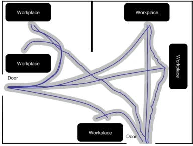
In the following sections, we are going to describe two kinds of techniques that cover most of the approaches in the area: grid models and cluster based models. In order to simplify the explanation, we will use a ?ctitious data set consisting of trajectories of people moving in a simpli?ed oEce environment (?g. 2.1). In order to increase readability, similar trajectories are supposed to go in the same direction. We are going to represent each trajectory di by a vector of con?gurations dti = {xti, yti} sampled at
regular intervals. Workplace Workplace Workplace W or kp la ce Workplace Door Door
Figure 2.1: Raw trajectories of people in an oEce environment
2.3.1
Grid Models
This term groups a number of proposals loosely based on Occupancy Grids [Elfes 89]. The main idea is to divide the working space using a tessellation (usually rectangular cells) and then, to calculate the probability for each of the resulting cells of being occupied. We are going to explain the technique proposed in [Kruse 96] which is representative of this kind of approach.
Learning Algorithm
The workspace is subdivided into rectangular cells c. For each of these cells we are going to calculate probabilities regarding both presence and direction of motion. We compute the probability of an object moving in one of eight directions P (c) where
{0,14 , ..., 7
4 }. We compute also the probability of an object resting in the same
grid for a while Ppartly(c). Having calculated that, the occupancy probability for the
cell Pocc(c) is given by the probability of resting in the same place plus the probability
of moving on each of the eight directions: Pocc(c) = Ppartly(c) + P (c).
To calculate P (c) and Ppartly(c) we proceed as follows: we observe the
environ-ment during a given time To at ?xed intervals t. For each cycle we update the values
for all the occupied cells by adding Tt
o to Ppartly(c) or one of the P (c) (depending on
the object’s motion) and then calculating Pocc(c).
W or kp la ce Door Door Workplace Workplace Workplace Workplace
Figure 2.2: Statistical Grid for example data
A representation of the resulting statistical grid for the example data is shown in ?g. 2.2. Darker cells have a higher Pocc(c) than lighter ones. P (c) is represented by
arrows.
Estimation Algorithm
In the proposal being explained, there is no explicit estimation process. The statistical grid is used to compute a collision probability ?eld (cp-?eld) which is directly used in motion planning to calculate the path with minimum collision probability using, a technique similar to that of gradient descent commonly used for potential ?elds.
Related Approaches
There exist many approaches which resembles the one presented here: In [Tadokoro 95], the statistical grid is manually introduced by a human and probabilities of occupa-tion of neighboring cells in the future are computed using Markov Chains to produce near future estimations. The work of [Tanaka 02] use very similar mechanics but it discretizes the space using a set of "feature points" instead of a grid.
Analysis
One important characteristic of most grid-based models is that they don’t produce "real" descriptive motion models: we obtain only a decomposition of the space with no explicit information about the paths themselves. This can be considered a drawback, nonetheless, grid approaches are useful in the sense that they provide information about regions and this information can be used even in the absence of sensorial input. This kind of models are useful, for example for motion preplanning; where we look for a general schedule to be followed before knowing actual environment con?guration and we want to avoid crowded regions.
The main advantage of grid models is its simplicity. These approaches are also capable of producing estimates of unobserved trajectories.
2.3.2
Cluster based Models
This family of approaches tries to group full trajectories in clusters which correspond to typical patterns. The main diEculty in this approach is that, although there is an extensive number of clustering algorithms (see [Kaufman 89] and [Jain 99]), most of them operate on vector spaces or need some kind of similarity measure and is not always easy to reformulate them in order to perform trajectory clustering. Here, we are going to discuss the approach followed by [Bennewitz 02].
Learning Algorithm
Both patterns and trajectories are represented as sequences of ?xed length T . As actual trajectory lengths may vary, they are normalized as follows: We choose T as the length of the longest trajectory. Trajectories of length T < T are extended to length T by appending the ?nal con?guration for T T times.
The approach assumes that an obstacle is engaged in one of K motion patterns. Each pattern, denoted by k with 1 k K is represented by T probability
distri-butions P (dti | tk). Those distributions represent the probability that an obstacle is at con?guration dti at time t given that it is engaged in motion pattern k.
Calculating the likelihood of a trajectory under the k-th motion model is straight-forward: P (di | k) = T t=1 P (dti| ti) (2.6)
In theory, to perform the clustering for a given training dataset D we only need to apply the expression 2.6 to calculate the likelihood of each one of the trajectories in D under each motion model and then assigning them to the most likely one. Un-fortunately, the parameters of the K models are unknown, hence, a way to estimate them is needed: Let’s assume that all the P (d | tk) functions can be represented
as multidimensional gaussians having a ?xed global known standard deviation , so that the only unknown parameters of our k models are the means of those
gaus-sians k = {µ1k, ..., µTk}. The approach aims to ?nd a maximum likelihood hypothesis
h = { 1, ..., K} which maximizes P (D | h). A trajectory di in D is assumed to
be-long to a single cluster; this fact is represented by a set of correspondence variables ci = {c1i, ..., cKi } for each di where cki = 1 if di belongs to cluster k and cki = 0
otherwise.
The values of ci are not included in the training data D, they are hidden variables.
It seems adequate to use the EM (Expectation-Maximization) algorithm which is a widely used approach to learning hidden variables. We are going to brieKy describe the algorithm, without going into details. We refer the interested reader to [Mitchell 97], for an excellent introduction to the subject, or [McLachlan 97] for a comprehensive resource. EM is an iterative algorithm that searches for a maximum likelihood hy-pothesis by repeating two steps:
1. Expectation. Calculate the expected value E[ck
i] of each hidden variable cki,
assuming the current hypothesis h.
2. Maximization. Calculate a new maximum likelihood hypothesis h = { 1, ..., K},
assuming that the value taken by each hidden variable cki is its expected value E[ck
i] calculated in step 1. Then replace the hypothesis h = h and iterate.
In ?gure 2.3 we can see a representation of the resulting clusters for the example data. The black lines are the values of µ, and the gray areas represent .
Estimation Algorithm
The estimation algorithm is simple: Expression 2.6 is applied to all K parameters , replacing T with the length of the partial trajectory being predicted. Then, the motion model having maximal probability is selected and output as an estimation.
Workplace Workplace Workplace W or kp la ce Workplace Door Door
Figure 2.3: Resulting Clusters for example data
One advantage of using EM is that the mean values found in the ?nal h are at the same time a representation of the cluster itself, which can be directly used to represent the predicted trajectory.
Related Approaches
An alternative proposal [GaJney 99] approximates trajectories using polynomials and then applying EM to ?nd the polynomial coeEcients. The same paper proposes also the use of EM to estimate trajectories using series of locally weighted functions.
Another interesting approach is presented in [Kruse 97]: they suggest represent-ing the trajectories by joined line segments obtained through recursive subdivision. Clustering is then performed on the segments instead of the whole trajectories. The resulting clusters are used for motion preplanning and to choose between reactive avoidance behaviors.
Analysis
In general, cluster based models are able to produce long-term, accurate predictions of trajectories that correspond to typical patterns. Even when these techniques are not able to uniquely determine the corresponding motion pattern, they are able to produce short-term estimates based on closest matching patterns. The main drawback of these techniques it that they fail to predict trajectories that don’t correspond to known motion patterns, this severely reduces their applicability to non structured environments where atypical trajectories are more likely to appear. On the other
hand, as they impose very few restrictions on the form of the trajectories, they are able to predict very complicated patterns. This makes them very useful in structured environments, where we can ?nd many common, but very complex trajectories.
One of the greatest strenghts of clustering based approaches is that they take into account not only the present state, but all information regarding past behavior, in this sense, they act as Markov Models of order Tobserved which is the number of
con?gurations in the observed trajectory.
2.3.3
Other Models
Other techniques are somewhat diEcult to classify. In [Boyd 00], space is modeled as a network of interconnected areas, and probabilities of transition between areas are calculated, this technique does not produce trajectory estimations but is useful to improve motion planning in highly structured environments. A technique wich classi?es trajectories using Kohonen Networks, but does not produce estimates is in-troduced in [Owens 00], It has been applied video surveillance to classify trajectories as "suspicious" or "dangerous", for example.
2.4
Data Clustering
We are going to discuss data clustering in this section because it is the basis for our proposed approach. Data Clustering aims to ?nd structure in raw data. The general idea is to partition an entire data set into meaningful groups called clusters. This suits well to our goal of ?nding general motion patterns in raw trajectory data coming from sensors. In this chapter, we present an overview of the ?eld as a background for our proposal.
2.4.1
De;nition of the problem
There are many de?nitions of what data clustering is, here we present a formal de?-nition adapted from [Fung 01]:
De;nition 1 Let D MN ×T be a set of data items, known as training data. D represents a set of N data items di in RT where each component of di is called a
feature and RT is called the feature space. The goal is to partition D into K groups Ck C where Ck is a particular group and C is the set of all the possible groups, such
that data items that belong to the same group are more similar to each other than to data items in di"erent groups. Each of the K groups is called a cluster. The result of the algorithm is an injective mapping D C of data items di to clusters Ck. We
There is a vast collection of clustering algorithms in the literature. Unfortunately, there is no technique that is universally applicable to all kind of problems, this is due to the fact that clustering algorithms often contain implicit assumptions about cluster shape and follow diJerent criteria [Jain 99]. Moreover, most algorithms need to know in advance the number K of clusters into which the data is going to be classi?ed. The problem of calculating K remains an open problem despite the existence of several proposals [Fraley ].
2.4.2
Similarity Measures
Similarity is a key concept of data clustering, and most techniques need some measure of similarity in order to work. This measure can be an explicit function of the data being analyzed, but it can also come from more subjective sources (i.e. human answers to a survey) The choice of such a measure is a critical aspect of a clustering solution. Due to the spatial nature of our problem, in this section we will focus on distance measures for patterns whose feature space is continuous
In general, for continuous feature spaces, the complementary concept of dissimi-larity is used by means of a distance measure de?ned in the feature space.
De;nition 2 Given a Feature space S, a distance or metric : S × S R is a function such that for all x, y, z S, all the following properties are veri ed:
(i) (x, x) = 0; (ii) (x, y) > 0, x = y; (iii) (x, y) = (y, x);
(iv) (x, z) (x, y) + (y, z)
Most clustering techniques can work with a submetric which doesn’t have to verify all of the properties.
One of the most used metrics is the Euclidean distance:
(di, dj) = ( T
t=1
(dti dtj)2)1/2= di dj 2
Which is a special case of the Minkowski Metric
(di, dj) = ( T
t=1
Minkowski Metrics presents some drawbacks, like the tendency of the largest-scaled features to dominate and distortion due to correlation among features. In order to alleviate this situation, a number of other metrics have been proposed like Mahalanobis Distance, HausdorJ Distance and many others [Mendelson 75].
Clustering algorithms can work in one of two ways (and sometimes in both of them): the ?rst mode is called model based clustering and, as its name suggest, it is based on the manipulation of cluster representations or models which are particular to the data being clustered. The second mechanism is known as pairwise clustering and it works using a table of dissimilarity values, consisting on the N (N 1)/2 pairwise distance values for the N patterns in the training set. Pairwise clustering does not calculate a representation of the clusters being created so, if such a representation is needed, a mechanism should be proposed to provide it.
2.4.3
Clustering Techniques
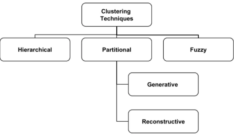
In this section, we brieKy explain a taxonomy of clustering techniques depicted in ?gure 2.4 and adapted from [Fung 01].and [Jain 99]. All the techniques can work both in model based and pairwise modes, with the exception of partitional generative methods, which are inherently model based.
Clustering Techniques Hierarchical Partitional Generative Reconstructive Fuzzy
Figure 2.4: Clustering Techniques
2.4.4
Hierarchical Clustering
The idea of hierarchical clustering is to produce a recursive representation of the groups. The output is a dendogram which is a tree-like structure whose root node
is a single cluster grouping all the observations and whose branches correspond to splittings of the parent clusters. Leafs are N singletons corresponding to all the data items in the training data set D.
An interesting property of dendograms is that they can be broken at diJerent sim-ilarity levels yielding to diJerent clusterings of the data. In ?gures 2.5 and 2.6) we can see the resulting clusters for a particular dissimilarity level chosen in the corresponding dendogram. A B C D E F G
Figure 2.5: Example Clusters (taken from [Jain 99])
Similarity
A B C D E F G
Hierarchical algorithms are called divisive if they start from a single cluster and then subsequently partition it. They are called agglomerative if they start from N clusters corresponding to each one of the training samples in D and then start to form fewer groups. Divisive and Agglomerative strategies correspond to top-down and bottom-up construction of the dendogram, respectively.
An agglomerative algorithm starts, as we said, with N clusters, one for each data item di Then, in the ?rst step, it joins the two closest clusters. As both clusters
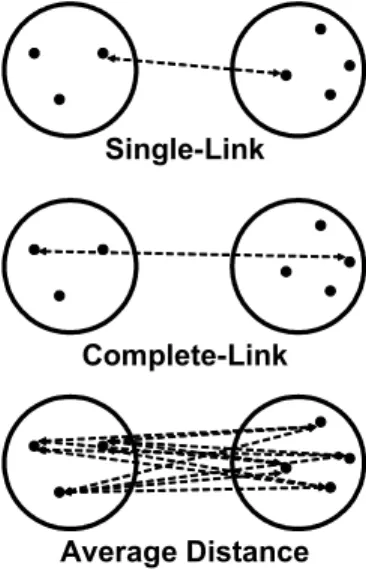
consist of only one data item, this means that the algorithm joins the pair of data items having smallest dissimilarity, leaving us with N 1 clusters. This process is repeated until we have only one cluster. However, this calls for a de?nition of distance between clusters having more than one item. In fact is the de?nition of this intercluster distance what distinguishes diJerent clustering algorithms [Kaufman 89]: Three of the most common measures, are nearest neighbor (single link), farthest neighbor (complete link) and average distance (see ?gure 2.7).
Single-Link
Complete-Link
Average Distance
Figure 2.7: Distance Between Clusters
2.4.5
Partitional Clustering
Partitional techniques output a single partition of training data instead of a hierarchi-cal clustering structure. The number of clusters K in the resulting partition is usually passed as a parameter to the clustering algorithm, the determination of K is a key de-cision and a diEcult problem itself. Partitional algorithms usually work by optimizing a criterion function de?ned either locally or globally respect to the training data D. Partitional techniques can be classi?ed as Generative or Reconstructive [Fung 01] (do
not confuse with Generative Motion Models).
Generative Algorithms
Generative algorithms assume that noisy data has been generated by K qualitatively similar, stochastic processes. [Fung 01] reformulates the problem as follows:
Consider a data set D = {d1, ..., dm} consisting of observations from a set of K
unknown distributions C1, ..., CK. If the density of an observation di with respect to
Cki is given by fk(di | ) for some unknown set of parameters . The probability
that di belongs to distribution Ck is denoted by cki. Since each observation is assumed
to belong to just one distribution, we have the constraint Kk=1cki = 1. The goal of generative algorithms is to ?nd the parameters and c that maximize the likelihood or, for analytical purposes, the log-likelihood:
L( , c) = N i=1 ln( K k=1 fk(di| )cki)
The Estimation-Maximization Algorithm ([McLachlan 97]) is often used to opti-mize this function.
One advantage exclusive of generative algorithms is that they calculate cluster representation and cluster assignation simultaneously.
Reconstructive Algorithms
This approach partitions the data into clusters by minimizing a cost function. The resulting assignment problem is a deterministic NP-hard combinatorial optimization problem [Buhmann 00]. The essential diJerence between the various types of re-constructive algorithms lies in the techniques used to model and minimize the cost function. Deterministic and stochastic approaches have been proposed. The classi-cal example of deterministic algorithms is the classic K-means ([MacQueen 67] and [Hartigan 78]) algorithm, which minimizes the within-groups sum of squares:
Cost(c) = K k=1 Ck i=1 Ck j=1,j=i cik cjk 2 Where ci
k represents the i-th member of cluster k. And c is a particular clustering.
An often used stochastic technique is Simulated Annealing [Dubes 89] A pairwise clustering algorithm based in Deterministic Annealing is proposed in [Hofmann 97].
2.4.6
Fuzzy Clustering
While in the other clustering approaches one object belongs to one and only one cluster, fuzzy clustering associates each pattern with every cluster using a membership function [Zadeh 65]. In other words, the output of such algorithm is a clustering, but not a partition. This kind of clustering produces a matrix U having N × K elements. [Jain 99] shows an iterated approach using the following fuzzy estimator:
E2(D, U ) = N i=1 K k=1 uji di ck 2
Proposed Approach
We propose an approach that aims at verifying the objectives ?xed in section 1.2, let’s recall them: We want a technique able of predicting motion of cars and pedestrians. This technique should verify the following properties:
1. It should produce estimations with a long Time Horizon.
2. It should be as general as possible and work with many diJerent kinds of objects. 3. It should be fast enough to give estimations in real time.
We have chosen to work on an estimation technique based on clustering. The rationale behind this decision obeys to the ?rst two objectives: After reviewing existing techniques, we have found that clustering based techniques provide the longest Time Horizon for their predictions; at the same time, almost no assumptions are made about motion characteristics, so that this kind of techniques can be applied in a general fashion.
Our method is similar in many ways to the approach described in subsection 2.3.2 that we are going to call EM estimator or EME. The main diJerence is that our approach is based on a dissimilarity metric which allows the use of pairwise clustering algorithms, so we decided to call it Pairwise Estimator or PWE.
Our method consists of two components (see subsection 2.3):
1. Learning. The goal of learning is to classify a training set of trajectories into K classes, corresponding to motion patterns. In our approach, the number and characteristics of the classes are not known a priori and they are discovered during the learning process.
2. Estimation. Our estimation process calculates, for a given observed fraction of trajectory opartial, its likelihood under each one of the K classes. The estimation
is the mean value of the class with maximum likelihood. Alternatively, we can present diJerent possibilities by returning the means of all the classes having likelihood greater or equal than a given threshold.
The details of the approach are presented in the following sections.
3.1
Learning Motion Patterns
In order to discover the typical motion patterns of obstacles we will use a dissimilarity measure (d1, d2) to construct a dissimilarity table which can be fed into any pairwise
clustering algorithm.
3.1.1
Similarity Measure
As our problem lies in the space-time domain, we consider an extension of the euclidean distance (see section 2.4.2). In order to apply our extension, we should introduce some conventions. A trajectory di of duration Ti can be viewed as a continuous, piecewise
de?ned function di(t) of time, where di(0) represents the beginning of the motion and
di(Ti) is the end of the motion. This function can be derived from descriptive models
assuming that any two subsequent con?gurations dti = {xti, yti} and dt+1i {xt+1i , yit+1} are joined by a straight line y = k1x + k0and calculating the values of k0 and k1 for
each of the Ti pieces. As a convention, we will say that di(t) = di(T ) for all t > Ti and
that the function is not de?ned for t < 0. The dissimilarity measure is:
(di, dj) = 1 max(Ti, Tj) max(T1,T2) t=0 (di(t) dj(t))2dt 1/2 (3.1)
Which is the average euclidean distance between the two functions. We have chosen the average because we want our measure to be independent of the length of the trajectories being compared.
3.1.2
Clustering Algorithm
The most important problem for running any clustering algorithm that uses K as a parameter is to estimate the value of K. EME solves this problem using the following method: it starts with one cluster and runs the algorithm. Whenever the EM has converged to a local maximum, it looks for trajectories with low data likelihood under the estimated models; when one such trajectory is found, a new model component is introduced that is initialized to that very trajectory. It also performs a redundancy
check for existing models: if global likelihood is not signi?cantly reduced by eliminating a model, then the model is reduced. After performing both tests, the EM algorithm is run again. The entire process is repeated until there is no change in the number of models.
Our approach follows a diJerent technique that we will proceed to explain.
Calculating the Number of Clusters
In order to estimate the value of K we have decided to use a clustering algorithm which does not need to know this value in advance. In particular, we are going to use a Complete-Link hierarchical agglomerative algorithm (see subsection 2.4.4). Nor-mally, this algorithm produces a structure providing diJerent clusterings at diJerent dissimilarity levels. In our case, we are going to output just one clustering, correspond-ing to a threshold chosen a priori. The complete link algorithm has the advantage of producing compact clusters and it guarantees that the dissimilarity between any two members of the same cluster is smaller or equal than the chosen threshold.
Complete-Link or CL is a pairwise clustering algorithm, so its input is a matrix of dissimilarities between clusters calculated using the expression 3.1. The matrix is initialized assuming that each individual trajectory di belongs to a diJerent cluster.
The algorithm is presented below.
Algorithm 3 Agglomerative Complete-Link Clustering WHILE min( ) < threshold DO
merge clusters corresponding to min( );
delete rows and columns in for the merged clusters; add entries in for the new cluster;
END
The creation of the new entries depends on the de?nition of distance between clus-ters. This de?nition is in fact what distinguishes diJerent agglomerative algorithms. For complete-link, the distance between clusters is the distance between the farthest neighboring trajectories (?gure 2.7).
Clustering with Deterministic Annealing [Hofmann 97]
Once we have an estimation of the value of K we can apply a pairwise clustering al-gorithm of our choice. An obvious question is immediately raised here: why do I want to cluster my data using another algorithm when I have already a clustering found by complete-link? The answer is that complete-link is based in a local objective function
(minimal dissimilarity ) and this local character frequently lends to "unnatural" clus-tering of data. Other approaches, like Deterministic Annealing try to optimize a global function and their results are often more satisfactory. At the end, we are not sure that the added clustering step will increase the performance of our estimation approach in a relevant way, so, in a later stage, we are going to evaluate the performance of Complete-Link vs. Deterministic Annealing.
Deterministic Annealing Clustering is based on statistical physics. It works with two sets of variables: 1) Mi , which has a value of 1 if sample i belongs to cluster -,
and 0 otherwise; and 2) .i which represents the average inKuence of exerted by all
Mk , k = i on the assignment Mi also known as mean-?eld. Both sets of variables are
interdependent and their values can be iteratively calculated in a way very similar to Estimation-Maximization. The variables are related by the two following expressions:
Mi = e i / K =1e i / (3.2) and .i = N 1 j=1,j=i Mj N k=1 Mk (di, dk) 1 2 Nj=1,j=i N j=1 Mj (dj, dk) (3.3)
As it name suggests, deterministic annealing uses a control value or temperature in a manner very similar to simulated annealing. It tracks solutions from high to low temperatures, where gradually more and more details of the original objective function appear. The complete resulting algorithm, as given in [Hofmann 97] is:
Algorithm 4 Deterministic Annealing Clustering INITIALIZE .i0 and Mi 0 RANDOMLY;
temperature 0;
WHILE > f inal
s 0; REPEAT
E-Like Step: estimate Mi s+1 as a function of . s i ;
M-Like Step: calculate .is+1 for given Mi s+1;
s s + 1; UNTIL all ( Mi s, . s i ) satisfy 3.3; / ; Mi 0 Mi s; . 0 i = . s i ;
3.1.3
Calculating Class Statistical Parameters
As we use only distance information for our clustering process, no cluster represen-tation is calculated for the resulting clusters. In this section, we propose a way to calculate the mean trajectory for each cluster and then the standard deviation for each cluster based on this mean value.
Calculating the Mean Trajectory
Let Ckbe a cluster having Nktrajectory functions di(t) | 1 i Nk, di(t) Ck, then
we de?ne the mean value of Ck as a function
µk(t) = 1 Nk
Nk
i=1
di(t) (3.4)
This expression is de?ned for t R+. As the t can take any positive real value, we need a way to calculate it without having to go through all the in?nite possible values of t. In order to do that, we are going to exploit the fact that all trajectory functions di(t) are piecewise ?rst-degree polynomials. Due to this fact, it suEces to
calculate µ(t) for values of t corresponding to the extreme points of each "piece" di,
the intermediate values are implicitly represented by the straight line equation. This leads naturally to the linear time-sweep algorithm which is presented below:
Algorithm 5 Time-Sweep Mean Trajectory Calculation events = ;
FOR every di in Ck DO
add all start and end times for pieces in di to events;
sort(events, ascending); µk= ;
FOR every t in events DO add µk(t) to µk;
In the preceding algorithm µk(t) represents a continuous function while µk repre-sents a descriptive model consisting on a discrete enumeration of con?gurations.
Calculating the Standard Deviation
Calculation of for cluster Ck is straightforward using the following expression:
k= 1 Nk Nk i=1 (di,µk)2 1/2 (3.5)
3.2
Estimating Trajectories
In order to estimate trajectories, we calculate the likelihood of a partially observed trajectory opartial under each one of the classes. To do that, we model classes as
gaussian sources with mean value and standard deviation as calculated in the previous section.
3.2.1
Partial Distance
As we are dealing with partial trajectories, we need to modify expression 3.1 to account for this. The modi?cation consists in measuring the distances respect to the duration of the partial trajectory:
partial(opartial, di) = 1 Tpartial Tpartial t=0 (opartial(t) di(t))2dt 1/2 (3.6)
Where partial, opartial and Tpartialare the partial distance, partially observed
tra-jectory, and duration of the partial tratra-jectory, respectively.
3.2.2
Calculating Likelihood
With the partial distance de?ned in expression 3.6, we can directly estimate likelihood of opartial under each cluster Ck.
P (opartial| Ck) = 1 2 k e 2 21 partial(opartial,µk) 2 (3.7) Once we have calculated the likelihood, we can choose to estimate the trajectory using the mean value of the cluster with maximal likelihood, or to present the diJerent possibilities having likelihood greater than a given threshold, for example.
3.2.3
Cluster Probability
An additional concept that can be introduced in our approach in latter works is the probability of occurrence of a cluster with respect to the other clusters. It allows us to make estimations in the absence of any sensorial input, answering questions like: I know that there is an object in the environment but I can’t see it, what’s the most likely trajectory for it? This probability can be approximated using the following expression:
P (Ck)
Nk
Where Nk is the number of trajectories in cluster k and ND is the total number of
trajectories in the data set D.
3.3
Analysis
As we said at the start of this chapter, we consider that Cluster Models have the advantage of providing longer Time Horizons because they produce estimates con-sisting in complete trajectories. Cluster Models made almost no assumptions about object’s motion and this yields to generality. On the other hand, Cluster Models have the important problem of not being able to predict trajectories that have not been observed.
Our approach is similar in form to EME, but it is based on pairwise clustering. In this sense, it is more general, because it allows choosing between many existing pairwise clustering algorithms while EME is tied to Expectation-Maximization. In addition, we consider that our approach presents the following advantages when compared to EME:
Independency of Motion Representation EME imposes three conditions on the training set: trajectories must be represented using a descriptive model, trajec-tories should be evenly sampled over time and all must have the same length. In contrast, PWE accept both generative and descriptive motion representations, samples can be uneven and length can be diJerent.
Lower computational complexity of the learning algorithm As we have said, the main diJerence between EME and PWE is that in PWE, we can choose a clustering algorithm. This allows us to use fast and simple computational algo-rithms as hierarchical clustering. As for EME, it is tied to EM, and it operates on very high dimensional vectors, this leads to great time and memory complex-ity and diEcults the application on large data sets.
Another practical problem of EME is that likelihood is computed as a multi-plication of probabilities for every component of a model: as probabilities are always <= 1, this can lead to numerical precision problems when the length of the trajectories exceeds a certain limit.
A drawback of our approach, when compared to EME, is that it requires and extra step to calculate cluster representations, while EME produces them directly as a part of its clustering algorithm. This drawback, however, is not very important, because the extra step is performed oSine.
Experimental Results
We have implemented our approach and tested it with simulated data. The algorithm proposed in [Bennewitz 02] was also implemented in order to compare it with our approach.
Java 1.4 was used as implementation language and tests were run in a PC having an 1.3 GHz Athlon microprocessor and 256 MB of RAM, the operating system was Windows XP.
The whole experimental process consisted of ?ve steps.
1. Generation of a Training Set of 1000 trajectories using a trajectory simulator. 2. Calculation of K using the complete-link algorithm. Clustering using
determin-istic annealing and Estimation-Maximization algorithms.
3. Generation of a Test set of 500 trajectories using a trajectory simulator.
4. Benchmark the training set against the three diJerent clustering algorithms and evaluate results using a performance metric.
Details on each one of the steps are provided in the following sections.
4.1
Generation of the Training Set
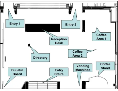
To test our approach, we used a simulator of the INRIA entry hall environment. In order to simulate trajectories, we de?ned a number of control points corresponding to important features of the environment; some of them are shown in ?gure 4.1.
We de?ned 32 trajectory prototypes consisting of sequences of control points to be traversed, the number of control points on each prototype ranged from 2 to 6. Trajectories were generated as follows:
Entry Stairs Directory Reception Desk Coffee Area 1 Coffee Area 2 Coffee Stand Vending Machines Bulletin Board Entry 1 Entry 2
Figure 4.1: The INRIA entry Hall
1. Actual points corresponding to each of the control points are generated using a bidimensional gaussian distribution with mean values corresponding to the center of the control point and equal to 20 cm.
2. Motion was simulated advancing in ?xed steps of 10 cm from the last control point in the direction of the next one, with a standard deviation of 0.3 rad. The next control point is considered to be reached when distance to it is less or equal than 10 cm.
3. Step 2 is repeated until the last control point is reached.
The 1000 trajectories in the training set D where generated choosing trajectory prototypes at random according to a given, not uniform probability distribution. The purpose of using such distribution is to simulate the fact that there are certain kinds of trajectories that occur more often that others.
4.2
Estimation of K and clustering
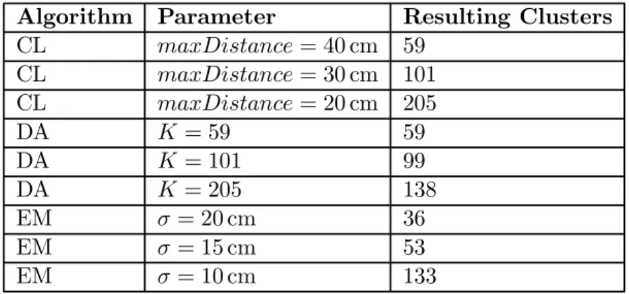
The complete link (CL) clustering algorithm was run against the data set using three diJerent distance thresholds: 20, 30 and 40 cm. The resulting clusterings where saved for benchmarking. The obtained values of K (59, 101 and 205, respectively) were fed into the Deterministic Annealing (DA) algorithm and the output clusterings were saved. It worths noting that DA sometimes produces clusters which have no assigned
elements. In our case, we simply ignored those clusters, hence, the actual numbers of clusters were 59, 99 and 138, respectively. For EME, we started with one cluster and used values of equal to 20, 15 and 10 cm, these values produced 36, 53 and 133 clusters, respectively. Results of this step are presented in table 4.1.
The values we have chosen for maxDistance and worth some discussion. We used three diJerent sets of values, because we know that these values aJect the number of clusters that we are going to obtain, and we are interested in studying the eJect of the number of clusters on estimation performance. We started by choosing the values for maxDistance knowing that they have a clear physical interpretation: for a given cluster Ck the maximal distance between two trajectories appertaining to the
cluster will not exceed maxDistance. As for the values of the parameter for EM, we have chosen, to base them on the values of maxDistance using the expression
= maxDistance2 .
Algorithm Parameter Resulting Clusters
CL maxDistance = 40 cm 59 CL maxDistance = 30 cm 101 CL maxDistance = 20 cm 205 DA K = 59 59 DA K = 101 99 DA K = 205 138 EM = 20 cm 36 EM = 15 cm 53 EM = 10 cm 133
Table 4.1: Clustering Results
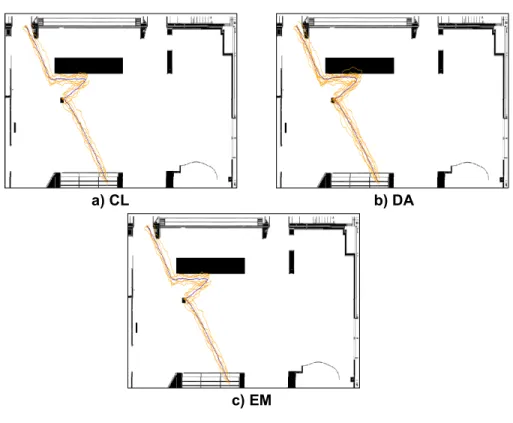
All three algorithm produced clusters which seemed reasonable when inspected visually, an example can be seen in ?gure 4.2 where similar clusters are displayed for the three algorithms. In each image, orange trajectories correspond to original trajectories in the data set, and the blue one corresponds to the cluster mean value.
4.3
Generation of the Test Set
The test set 4 of 500 trajectories was generated in an analogous way to the one used for generating training data. The same parameters and trajectory prototypes were used.
a) CL b) DA
c) EM
Figure 4.2: Examples of generated clusters for the three algorithms.
4.4
Benchmarking
In order to compare the diJerent approaches and clustering algorithms, we de?ned a simple performance metric. Its inputs are a given clustering C, the test set 4, and the percentage in length of each trajectory in the test set that will be used to ?nd an estimate.
The metric is calculated using the following algorithm, where N! is the total
num-ber of trajectories in the test set.
Algorithm 6 Performance metric
Function PerformanceMetric( 4, C, percentage) result 0;
FOR each trajectory 4i in the test set 4 DO calculate 4percentagei ;
nd the cluster Ck with max likelihood for 4percentagei ;
result result + (4i, µk); END FOR
The metric is basically the average dissimilarity between the real trajectories in the test set and the estimations obtained using a given percentage of those trajecto-ries. Lower values are better then higher ones. Tests where performed against the 9 clusterings listed in table 4.1. General results are shown in ?gure 4.3, there we can see, for example, that the clustering produced using the EM algorithm with = 20 and having K = 36, scored a value of 48.71 when estimations where calculated using 30% of the length of the observed (test set) trajectories.
General Comparative 0 10 20 30 40 50 60 70 80 90
Length of Observed Trajectory (%)
M ea n D is si m il ar it y CL 40 K=59 69.88 55.05 43.2 33.58 29.1 22.29 19.31 18.52 CL 30 K=101 70.72 48.71 39.25 32.15 27.65 19.57 16.66 15.84 CL 20 K=205 80.67 54.41 43.6 29.58 23.88 16.66 14.68 13.72 DA 59 K=59 64.94 48.47 38.74 32.81 30.63 24.03 20.48 19.46 DA 101 K=99 59.41 43.8 35.12 27.16 25.58 19.37 16.9 16.03 DA 205 K=138 58.29 45.5 39.71 28.62 25.54 19.08 15.89 15.36 EM 20 K=36 72.08 55 48.71 39.42 36.06 24.12 21.73 21.01 EM 20 K=36 83.62 56.78 46.76 42.45 36.85 26.36 19.85 18.86 EM 10 K=133 79.81 50.5 38.37 32.01 30.23 17.56 15.83 15.24 10% 20% 30% 40% 50% 60% 70% 80%
a. b.
c. d.
Figure 4.4: Trajectory Estimation for DiJerent Instants
4.5
Graphical Representation of Estimation
We have implemented a GUI that displays results of the estimation process as it evolves over time (?gure 4.4). In order to do this, likelihood is calculated for all clusters using expression 3.7. The GUI displays the average values of the clusters having a likelihood greater than a given threshold; most likely estimates are shown in dark red, less likely ones are lighter. The object’s position is represented by a black circle, the observed trajectory is shown with a black line. Future motion is depicted in blue.
As can be seen in (?gure 4.4), even if motion estimates change over time, near future motion is accurately estimated, except for the initial con?guration, which can not be very discriminating because not much information is available.
4.6
Analysis
When observed using the GUI, predictions based on all the 9 clusterings seem to be "reasonable" and it is diEcult to make an evaluation using this empirical data. In contrast, numerical results presented in ?gure 4.3 shows very interesting results. In the ?rst place, we can see that quality of estimations seems to converge as the length
of observed trajectory grows, which seems reasonable: we expect precision to increase as more information is used in the estimation process, and, at the same time, we know that ?nal precision will be limited by the number of available clusters.
We can see also that, in general, DA performs better than the two other algorithms (see ?gure 4.5) especially for values of observed length smaller than 40%. We can interpret this as saying that DA seems to produce clusterings that represent real motion more accurately than the other two algorithms.
Comparative for K=101
0 50 100
Length of Observed Trajectory (%)
M ea n D is si m il ar it y CL 30 K=101 70.7 48.7 39.3 32.2 27.7 19.6 16.7 15.8 DA 101 K=99 59.4 43.8 35.1 27.2 25.6 19.4 16.9 16 EM 15 K=53 83.6 56.8 46.8 42.5 36.9 26.4 19.9 18.9 10% 20% 30% 40% 50% 60% 70% 80% Comparative for K=101 0 50 100
Length of Observed Trajectory (%)
M ea n D is si m il ar it y CL 30 K=101 70.7 48.7 39.3 32.2 27.7 19.6 16.7 15.8 DA 101 K=99 59.4 43.8 35.1 27.2 25.6 19.4 16.9 16 EM 15 K=53 83.6 56.8 46.8 42.5 36.9 26.4 19.9 18.9 10% 20% 30% 40% 50% 60% 70% 80% Comparative for K=205 0 50 100
Length of Observed Trajectory (%)
M ea n D is si m il ar it y CL 20 K=205 80.7 54.4 43.6 29.6 23.9 16.7 14.7 13.7 DA 205 K=138 58.3 45.5 39.7 28.6 25.5 19.1 15.9 15.4 EM 10 K=133 79.8 50.5 38.4 32 30.2 17.6 15.8 15.2 10% 20% 30% 40% 50% 60% 70% 80%
Figure 4.5: Results by Number of Clusters
In ?gure 4.6, we present the processing times for the three clusterings performed for each algorithm in ascending order with respect to the number of clusters. CL is the best absolute performer; in addition we can see that clustering time is practically independent of the number of clusters. As a matter of fact, most of the time was consumed calculating the dissimilarity table. Next in performance is Expectation-Maximization, whose longer time was around half an hour for 133 clusters. Finally, we can see that DA is much slower than the other two algorithms. Thus, the precision of DA seems to have a cost, however, it worths noting that clustering is an oJ-line process which is only run once.
dis-similarity table uses memory proportional to the square of the size of the training set, this limits the number of samples that can be actually used in learning.
Clustering Times 0 500 1000 1500 2000 2500 3000 3500 4000 4500 T im e (S ec o n d s) CL DA EM CL 262 262 263 DA 776 2912 4127 EM 480 754 1762 1 2 3
Figure 4.6: Clustering times
We can conclude that, according to the tests performed using our benchmarking criterion, PWE performs better than EME in producing long term estimations of the motion of objects, and that its only drawback is that the number of samples in the training set is limited by the amount of memory available.
As for our third goal, the possibility of using our approach in real time, we should say that in our tests the maximum time needed for estimation is slightly smaller than one second for a trajectory having 120 points. This, is not acceptable for use in real time applications, however, a drastic improvement can be obtained by incrementally calculating likelihoods for each new observation using the result obtained for the last observation. With this simple optimization, the maximal estimation time would be reduced to about 1/100 of a second which is suitable for most real time applications dealing with humans and cars.
To conclude this chapter, we are going to present some early results obtained using real data. The trajectories were captured using a vision system developed by the team PRIMA of the INRIA using a camera placed in the entry hall of the laboratory (?gure 4.7). Trajectory coordinates where transformed from the image to the hall’s plan by correcting the distortion and then applying an homography.
Some of the resulting clusters can be seen in ?gure 4.8. As we have said, these are only early results: we are still working in issues like ?ltering out artifacts that appear due to light reKecting on the Koor. In any case, we expect to solve this issues in the short term in order to test our estimation technique both in the entry hall and in the lab’s parking lot.
Figure 4.7: The Camera View
Conclusions
The work presented in this document deals with the problem of predicting future motion of objects using knowledge about past and present motion. We are particularly interested in motion prediction for pedestrians and vehicles.
5.1
Summary and Contributions
We have presented an introduction to the ?eld and proposed a classi?cation of exist-ing techniques based in motion representation. We have reviewed the two resultexist-ing categories: Generative and Descriptive Models. We also have outlined data clustering, which is the basis for our approach.
We have proposed and implemented a motion estimation technique called Pairwise Estimation (PWE) based on clustering. As most estimation techniques based on descriptive models, our approach is de?ned by two processes: learning and estimation:
1. For the learning stage, we propose a distance metric that can be used to perform trajectory clustering using any existing pairwise clustering algorithm. According to our knowledge, this is a novel approach to trajectory clustering. We also describe how to use the Complete-Link clustering algorithm in order to calculate the number of clusters. We propose a simple algorithm to calculate the mean value for a cluster of trajectories. This mean trajectory is then used to calculate the standard deviation for each cluster.
2. For the estimation stage, we propose a simple way to calculate the likelihood that a partially observed trajectory corresponds to a certain cluster. This likelihood, can be calculated for each cluster, obtaining in this way a probabilistic represen-tation of motion. We can also simply select the most likely pattern obtaining in this way a deterministic prediction.


![Figure 2.6: Corresponding Dendogram (taken from [Jain 99])](https://thumb-eu.123doks.com/thumbv2/123doknet/12145164.311330/24.918.282.630.760.1039/figure-corresponding-dendogram-taken-from-jain.webp)