HAL Id: hal-01387293
https://hal.inria.fr/hal-01387293
Submitted on 25 Oct 2016
HAL is a multi-disciplinary open access
archive for the deposit and dissemination of
sci-entific research documents, whether they are
pub-lished or not. The documents may come from
teaching and research institutions in France or
abroad, or from public or private research centers.
L’archive ouverte pluridisciplinaire HAL, est
destinée au dépôt et à la diffusion de documents
scientifiques de niveau recherche, publiés ou non,
émanant des établissements d’enseignement et de
recherche français ou étrangers, des laboratoires
publics ou privés.
Importance Sampling for Stochastic Timed Automata
Cyrille Jegourel, Kim Guldstrand Larsen, Axel Legay, Marius Mikučionis,
Danny Poulsen, Sean Sedwards
To cite this version:
Cyrille Jegourel, Kim Guldstrand Larsen, Axel Legay, Marius Mikučionis, Danny Poulsen, et al..
Importance Sampling for Stochastic Timed Automata. Dependable Software Engineering: Theories,
Tools, and Applications, Nov 2016, Beijing, China. �hal-01387293�
Importance Sampling for Stochastic Timed
Automata
Cyrille Jegourel1, Kim G. Larsen2, Axel Legay2,3, Marius Mikuˇcionis2,
Danny Bøgsted Poulsen2, and Sean Sedwards3
1
National University of Singapore
2
Department of Computer Science, Aalborg University, Denmark
3
INRIA Rennes – Bretagne Atlantique, France
Abstract. We present an importance sampling framework that
com-bines symbolic analysis and simulation to estimate the probability of rare reachability properties in stochastic timed automata. By means of symbolic exploration, our framework first identifies states that cannot reach the goal. A state-wise change of measure is then applied on-the-fly during simulations, ensuring that dead ends are never reached. The change of measure is guaranteed by construction to reduce the variance of the estimator with respect to crude Monte Carlo, while experimental results demonstrate that we can achieve substantial computational gains.
1
Introduction
Stochastic Timed Automata [7] extend Timed Automata [1] to reason on the stochastic performance of real time systems. Non-deterministic time delays are refined by stochastic choices and discrete non-deterministic choices are refined by probabilistic choices. The semantics of stochastic timed automata is given in terms of nested integrals over products of uniform and exponential distributions. Abstracting from the stochasticity of the model, it is possible to find the symbolic paths reaching a set of goal states, but solving the integrals to calculate the probability of a property becomes rapidly intractable. Using a similar abstraction it is possible to bound the maximum and minimum probabilities of a property, but this can lead to results such as the system could work or fail with high
probability. Our goal is to quantify the expectation of rare behaviour with specific
distributions.
A series of works [7, 5, 3, 4] has developed methods for analysing Stochastic Timed Automata using Statistical Model Checking (SMC) [18]. SMC includes a collection of Monte Carlo techniques that use simulation to avoid “state space ex-plosion” and other intractabilities encountered by model checking. It is typically easy to generate sample executions of a system, while the confidence of estimates increases with the number of independently generated samples. Properties with low probability (rare properties) nevertheless pose a challenge for SMC because the relative error of estimates scales inversely with rarity. A number of standard variance reduction techniques to address this have been known since the early days of simulation [11]. The approach we present here makes use of importance
a probabilistic measure that makes the rare event more likely to occur. An un-biased estimate is achieved by compensating for the change of measure during simulation.
Fig. 1: A rare event of reachingAdue to timing constraints. Our model may include rarity arising from explicit
Markovian transitions, but our main contribution is ad-dressing the more challenging rarity that results from the intersection of timing constraints and continuous distribu-tions of time. To gain an intuition of the problem, consider the example in Fig. 1. The automaton first chooses a delay uniformly at random in [0, 106] and then selects to either
go to A or B. Since the edge to A is only enabled in the interval [106− 1, 106], reachingAconstitutes a rare event with probability∫10 6 106−110−6· 1 2dt = 1 2· 10−6.
The probability theory relating to our model has been considered in the framework of generalised semi Markov processes, with related work done in the context of queueing networks. Theory can only provide tractable analytical so-lutions for special cases, however. Of particular relevance to our model, [17] pro-poses the use of state classes to model stochastic distributions over dense time, but calculations for the closely related Duration Probabilistic Automata [14] do not scale well [12]. Monte Carlo approaches provide an approximative alternative to analysis, but incur the problem of rare events. Researchers have thus turned to importance sampling. In [19] the authors consider rare event verification of a model of stochastic hybrid automata that shares a number of features in com-mon with our own model. They suggest using the cross-entropy method [16] to refine a parametrised change of measure for importance sampling, but do not provide a means by which this can be applied to arbitrary hybrid systems.
Our contribution is an automated importance sampling framework that is integrated into Uppaal SMC and applicable to arbitrary time-divergent priced timed automata [7]. By means of symbolic analysis we first construct an exhaus-tive zone-based reachability graph of the model and property, thus identifying all “dead end” states that cannot reach a satisfying state. Using this graph we generate simulation traces that always avoid dead ends and satisfy the property, applying importance sampling to compensate estimates for the loss of the dead ends. In each concrete state we integrate over the feasible times of enabled ac-tions to calculate their total probabilities, which we then use to choose an action at random. We then choose a new concrete vector of clock values at random from the feasible times of the chosen action, using the appropriately composed distribution. All simulated traces reach satisfying states, while our change of measure is guaranteed by construction to reduce the variance of estimates with respect to crude Monte Carlo. Our experimental results demonstrate substantial reductions of variance and overall computational effort.
The remainder of the paper is as follows. Section 2 and Section 3 provide back-ground: Section 2 recalls the basic notions of importance sampling and Section 3 describes Stochastic Timed Automata in terms of Stochastic Timed Transition Systems. We explain the basis of our importance sampling technique in Section 4 and describe how we realise it for Stochastic Timed Automata in Section 5. In Section 6 we present experimental results using our prototype implementation
in Uppaal SMC and then briefly summarise our achievements and future work in Section 7.
2
Variance Reduction
Let F be a probability measure over the measurable set of all possible executions
ω∈ Ω. The expected probability pφof property φ is defined by
pφ= ∫
Ω
1φdF, (1)
where the indicator function 1φ : Ω → {0, 1} returns 1 iff ω satisfies φ. This leads to the standard (“crude”) unbiased Monte Carlo estimator used by SMC:
pφ≈ 1 N N ∑ i=1 1φ(ωi), (2)
where each ωi∈ Ω is selected at random and distributed according to F , denoted
ωi ∼ F . The variance of the random variable sampled in (2) is given by
σ2crude= ∫ Ω (1φ− pφ)2dF = ∫ Ω 1φdF− (pφ)2 (3)
The variance of an N -sample average of i.i.d. samples is the variance of a single sample divided by N . Hence the variance of the crude Monte Carlo estimator (2) is σcrude2 /N and it is possible to obtain more confident estimates of pφ by increasing N . However, when pφ ≈ 0, i.e., φ is a rare property, standard con-centration inequalities require infeasibly large numbers of samples to bound the
relative error.
In this work we use importance sampling to reduce the variance of the random variable from which we sample, which then reduces the number of simulations necessary to estimate the probability of rare properties. Referring to the same probability space and property used in (1), importance sampling is based on the integral pφ= ∫ Ω 1φ dF dGdG, (4)
where G is another probability measure over Ω and dF/dG is called the likelihood
ratio, with 1φF absolutely continuous with respect to G. Informally, this means that ∀ω ∈ Ω, dG(ω) = 0 =⇒ 1φdF (ω) = 0. Hence 1φ(ω)dF (ω)/dG(ω) > 0 for all realisable paths under F that satisfy φ and is equal to 0 otherwise.
The integral (4) leads to the unbiased importance sampling estimator
pφ≈ 1 N N ∑ i=1 1φ(ωi) dF (ωi) dG(ωi) , ωi∼ G. (5)
In practice, a simulation is performed under measure G and if the resulting trace satisfies φ, its contribution is compensated by the likelihood ratio, which
is calculated on the fly. To reduce variance, the intuition is that G is constructed to make traces that satisfy φ more likely to occur in simulations.
The variance σis2 of the random variable sampled by the importance sampling estimator (4) is given by σis2 = ∫ Ω ( 1φ dF dG− pφ )2 dG = ∫ Ω 1φ ( dF dG )2 dG− (pφ)2 (6)
If F = G, the likelihood ratio of realisable paths is uniformly equal to 1, (4) reduces to (1) and (6) reduces to (3). To ensure that the variance of (5) is less than the variance of (2) it is necessary to make σis2 < σcrude2 , for which it is sufficient to make dF/dG < 1,∀ω ∈ Ω.
Lemma 1. Let F, G be probability measures over the measurable space Ω, let 1φ : Ω → {0, 1} be an indicator function and let 1φF be absolutely continuous
with respect to G. If for all ω∈ Ω, 1φ(ω)·
dF (ω)
dG(ω) ≤ 1 then σ 2
is≤ σcrude2 .
Proof. From the definitions of σ2
crude (3) and σ 2 is (6), we have σ2is≤ σ2crude ⇐⇒ ∫ Ω 1φ ( dF dG )2 dG− (pφ)2≤ ∫ Ω 1φdF− (pφ)2,
where pφ is the expectation of 1φF . Noting that (pφ)2 is outside the integrals and common to both sides of the inequality, we conclude
σ2is≤ σ2crude ⇐⇒ ∫ Ω 1φ dF dGdF ≤ ∫ Ω 1φdF.
Hence, given 1φ ∈ {0, 1}, to ensure σ2is ≤ σ2crude it is sufficient that 1φ(ω)·
dF (ω)
dG(ω) ≤ 1, ∀ω ∈ Ω.
3
Timed Systems
The modelling formalism we consider in this paper is a stochastic extension of Timed Automata [1] in which non-deterministic time delays are refined by stochastic choices and non-deterministic discrete choices are refined by proba-bilistic choices. Let Σ = Σ!∪ Σ? be a set of actions split into output (Σ!) and input (Σ?). As usual we assume there is a one-to-one-mapping between input actions and output actions. We adopt the scheme that a! is an output action and a? is the corresponding input action.
Definition 1 (Timed Transition System). A timed transition system over actions Σ split into input actions Σ? and output actions Σ! is a tuple L =
(S, s0,→, AP, P) where 1) S is a set of states, 2) s0 is the initial state, 3)→⊆ S× (Σ ∪ R≥0)× S is the transition relation, 4) AP is a set of propositions and
For shorthand we write s −→ sa ′ whenever (s, a, s′)∈→. Following the composi-tional framework laid out by David et al. [6] we expect timed transition systems to be action-deterministic i.e. if s−→ sa ′ and s−→ sa ′′ then s′= s′′ and we expect them to be input-enabled meaning for all input actions a? ∈ Σ? and all states
s there exists s′ such that s −→ sa? ′. Let s, s′ ∈ S be two states then we write
s→∗s′ if there exists a sequence of transitions such that s′is reachable and we write s ̸→∗ s′ if s′ is not reachable from s. Generalising this to a set of states G⊆ S, we write s →∗G if there exists s′ ∈ G such that s →∗s′ and s̸→∗G if for all s′∈ G, s ̸→∗s′.
A run over a timed transition system L = (S, s0,→, AP, P) is an
alternat-ing sequence of states, reals and output actions, s0d0a0!s1d1a1! . . . such that si
di
−→−−→ sai!
i+1. We denote by Ω(L) the entire set of runs over L. The set of propositional runs is the set ΩAP(L) = {P(s
0)d0, . . .|s0d0a0!∈ Ω(L)}.
Several Timed Transition SystemsL1. . .Ln, Li = (Si, s0i,→i, APi, Pi), may be composed in the usual manner. We denote this byL = L1|L2| . . . |Ln and for a state s = (s1, s2, . . . , sn) ofL we let s[i] = si.
Timed Automata Let X be a finite set of variables called clocks. A valuation over
a set of clocks is a function v : X → R≥0 assigning a value to each clock. We denote by V (X) all valuations over X. Let v∈ V (X) and Y ⊆ X then we denote by v[Y ] the valuation assigning 0 whenever x∈ Y and v(x) whenever x /∈ Y . For a value d∈ R≥0 we let (v + d) be the valuation assigning v(x) + d for all x∈ X. An upper bound (lower bound ) over a set of clocks is an element x ▹ n (x ◃ n) where x∈ X, n ∈ N and ▹ ∈ {<, ≤} (◃ ∈ {>, ≥}). We denote the set of finite conjunctions of upper bounds (lower bounds) over X byB▹(X) (B◃(X)) and the set of finite conjunctions over upper and lower bounds byB(X). We write v |= g whenever v ∈ V (X) satisfies an element g ∈ B(X). We let v0 ∈ V (X) be the
valuation that assigns zero to all clocks.
Definition 2. A Timed Automaton over output actions Σ!and input actions Σ?
is a tuple (L, ℓ0, X, E, Inv) where 1) L is a set of control locations, 2) ℓ0 is the initial location, 3) X is a finite set of clocks, 4) E⊆ L×B◃(X)×(Σ
!∪Σ?)×2
X×L
is a finite set of edges 5) Inv : L→ B▹(X) assigns an invariant to locations. ⊓⊔ The semantics of a timed automatonA = (L, ℓ0, X, E, Inv) is a timed transition
systemL = (S, s0,→, L, P) where 1) S = L × V (X), 2) s0= (ℓ
0, v0), 3) (ℓ, v)
d
−→
(ℓ, (v + d)) if (v + d)|= Inv(ℓ), 4) (ℓ, v)−→ (ℓa ′, v′) if there exists (ℓ, g, a, r, ℓ′)∈ E such that v|= g, v′ = v[r] and v′ |= Inv(ℓ′) and 5) P((ℓ, v)) ={ℓ}.
3.1 Stochastic Timed Transition System
A stochastic timed transition system (STTS) is a pair (L, ν) where L is a timed transition system defining allowed behaviour and ν gives for each state a density-function, that assigns densities to possible successors. Hereby some behaviours may, in theory, be possible forL but rendered improbable by ν.
Definition 3 (Stochastic Timed Transition System). Let L = (S, s0,→ , AP, P) be a timed transition system with output actions Σ! and input actions Σ?. A stochastic timed transition system over L is a tuple (L, ν) where ν : S →
R≥0× Σ!→ R≥0 assigns a joint-delay-action density where for all states s∈ S, 1)∑a!∈Σ
!
(∫R
≥0ν(s)(t, a!) dt) = 1 and 2) ν(s)(t, a!)̸= 0 implies s
t
− →a!
−→. ⊓⊔
1) captures that ν is a probability density and 2) demands that if ν assigns a non-zero density to a delay-action pair then the underlying timed transition system should be able to perform that pair. Note that 2) is not a bi-implication, reflecting that ν is allowed to exclude possible successors ofL.
Forming the core of a stochastic semantics for a stochastic timed transition system T = ((S, s0,→, AP, P), ν), let π = p
0I0p1I1p2. . . In−1pn be a cylinder construction where for all i, Iiis an interval with rational end points and pi⊆ AP. For a finite run ω = p′1d1p′2. . . dn−1pn we write ω |= π if for all i, di ∈ Ii and
p′i= pi. The set of runs within π is then C(π) ={ωω′∈ ΩAP(T) | ω |= π}. Using the joint density, we define the measure of runs in C(π) from s recursively:
Fs(π) = (p0= P(s))· ∫ t∈I0 ∑ a!∈Σ! ( ν(s)(t, a!)· F[[s]d]a!(π1) ) dt, where π1 = p
1I1. . . pn−1pn, base case Fs(p) = (PT(s) = (p)) and [s]a is the uniquely defined s′ such that s−→ sa ′. With the cylinder construction above and the probability measure F , the set of runs reaching a certain proposition p within a time limit t, denoted as♢≤tp, is measurable.
(a) A
(b) B
Fig. 2: Two Stochastic Timed Automata.
Stochastic Timed Automata (STA) Following [7], we
associate to each state, s, of timed automaton A = (L, ℓ0, X, E, Inv) a delay density δ and a probability
mass function γ that assigns a probability to out-put actions. The delay density is either a uniform distribution between the minimal delay (dmin) be-fore a guard is satisfied and maximal delay (dmax) while the invariant is still satisfied, or an exponen-tial distribution shifts dmin time units in case no invariant exists. The γ function is a simple dis-crete uniform choice of all possible actions. For-mally, let dmin(s) = min{d|s
d
−→a!
−→ for some a!} and dmax(s) = sup{d|s
d
−
→} then δ(s)(t) = 1
dmax(s)−dmin(s)
if dmax(s) ̸= ∞ and δ(s)(t) = λ · e−λ(t−dmin(s), for
a user specified λ, if dmax(s) = ∞. Regarding output actions, let Act(s) =
{a!|s a!
−→}, then γ(s)(a!) = 1
|Act| for a! ∈ Act. With δ and γ at hand we de-fine the stochastic timed transition system for A with underlying timed tran-sition system L as TA = (L, δ • γ), where δ • γ is a composed joint-delay-density function and (δ• γ)(s)(t, a!) = δ(s)(t) · γ([s]t)(a!). Notice that for any
t,∑a!∈Σ
!ν(s)(t, a!) = δ(s)(t). In the remainder we will often write a stochastic
Example 1. Consider Fig. 2 and the definition of δA and γA in the initial state
(A.I,x=0). By definition we have γA((I,x=0)(t)(a!) = 1 for t ∈ [90, 100] and δA(I,x=0)(t) = 1001−90 for t ∈ [90, 100]. Similarly for the B component in the
state (B.I,x=0) we have γB((I,x=0)(t)(b!) = 1 if t∈ [0, 100] and zero otherwise
and δB(I,x=0)(t) =1001−0 if t∈ [0, 100] and zero otherwise.
3.2 Composition of Stochastic Timed Transitions Systems
Following [7], the semantics of STTS is race based, in the sense that each com-ponent first chooses a delay, then the comcom-ponent with the smallest delay wins the race and finally selects an output to perform. For the remainder we fix
Ti = (Li, νi) where Li = (Si, s0i,→i, APi, Pi) is over the output actions Σ!i and
the common input actions Σ?.
Definition 4. LetT1,T2, . . . ,Tn be stochastic timed transition systems with
dis-joint output actions. The composition of these is a stochastic timed transition systemJ = (L1|L2| . . . |Ln, ν) where ν(s)(t, a!) = νk(s[k])(t, a!)· ∏ j̸=k ∫ τ >t ∑ b!∈Σj! νj(s[j])(τ, b!) dτ for a! ∈ Σk !.
The race based semantics is apparent from ν in Definition 4, where the kth component chooses a delay t and action a! and each of the other components independently select a τ > t and an output action b!. For a composition of Stochastic Timed Automata we abstract from the losing components’ output actions and just integrate over δ, as the following shows. Let J = (L, ν) be a composition of stochastic timed transition systems, T1,T2, . . . ,Tn, and let for all i, Ti = (Li, δi • γi) originate from a timed automaton. Let a! ∈ Σ!k, then ν(s)(t, a!) is given by δk(s[k])(t)· γk(sk)(t)(a!)· ∏ j̸=k ∫ τ >t ∑ b!∈Σj ! δj(s[j])(τ )γj(s[j])(τ )(b!) dτ = δk(s[k])(t)· ∏ j̸=k (∫ τ >t δj(s[j])(τ ) dτ ) · γk(s[k])(t)(a!). The term δk(s[k])(t)· ∏ j̸=k (∫ τ >tδj(s[j])(τ ) dτ )
is essentially the density of the
kth component winning the race with a delay of t. In the sequel we let κδ k(t) = δk(s[k])(t)· ∏ j̸=k (∫ τ >tδj(s[j])(τ ) dτ ) .
Example 2. Returning to our running example of Fig. 2, we consider the
joint-delay density of the composition in the initial state s = (sA, sB), where sA =
(I, x = 0) and sB= (I, x = 0). Applying the definition of composition we see that
νA|B(s)(t, c!) = 1 100−90 · 100−t 100−0· 1 if t ∈ [90, 100] and c! =a! 1 100−0· 1 if t∈ [0, 90[ 1 100−0· 100−t 100−90· 1 if t ∈ [90, 100] } and c! =b!.
4
Variance Reduction for STTS
For a stochastic timed transition systemT = ((S, s0,→, AP, PL), ν) and a set of goal states G ⊆ S we split the state space into dead ends (⌢G) and good ends
(⌣G) i.e. states that can never reach G and those that can. Formally,
⌢G={s ∈ S | s ̸→∗G} and ⌣G={s ∈ S | s →∗G}.
For a state s, let ActG,t(s) = {a! | [[s]t]a! ∈⌣G} and DelF(s) = {d | [s]d ∈⌣G ∧ActG,d(s)̸= ∅}. Informally, ActG,t(s) extracts all the output actions that after
a delay of t will ensure having a chance to reach G. Similarly, DelG(s) finds all
the possible delays after which an action can be performed that ensures staying in good ends.
Definition 5 (Dead End Avoidance). For a stochastic timed transition sys-tem T = ((S, s0,→, AP, P), ν) and goal states G, we define an alternative dead end-avoiding stochastic timed transition system as any stochastic timed transi-tion system ´T = ((S, s0,→, AP, P), ´ν) where if ´ν(s)(t, a!) ̸= 0 then a! ∈ Act
G,t(s). ⊓ ⊔
Recall from Lemma 1 in Section 2 that in order to guarantee a variance reduction, the likelihood ratio should be less than 1. Let T = ((S, s0,→, AP, P
L), ν) be a stochastic timed transition system, let G ⊆ S be a set of goal states and let ´T = ((S, s0,→, AP, P
L), ´ν) be a dead end-avoiding alternative. Let ω =
s0, d0, a0!s1, . . . dn−1an−1!sn be a time bounded run, then the likelihood ratio of
ω sampled under ´T is dT(ω) d ´T(ω) = ν(s0)(d0, a0!) ´ ν(s0)(d0, a0!)· ν(s1)(d1, a1!) ´ ν(s1)(d1, a1!) . . .ν(sn−1)(dn−1, an−1!) ´ ν(sn−1)(dn−1, an−1!) Clearly, if for all i, ν(si)(di, ai!)≤ ´ν(si)(di, ai!) then dd ´T(ω)
T(ω)≤ 1. For a stochastic timed transition system (L, ν = δ • γ) originating from a stochastic timed au-tomaton we achieve this by proportionalising δ and γ with respect to good ends, i.e. we use ˜υ = ˜δ• ˜γ where
˜
δ(s)(t) = ∫ δ(s)(t)
DelG(s)δ(s)(τ ) dτ
and ˜γ(s)(t)(a!) = ∑ γ(s)(t)(a!)
b!∈ActG,t(s)γ(s)(t)(b!) .
Lemma 2. Let T = (L, ν = δ • γ) be a stochastic timed transition system from
a stochastic timed automata, let G be a set of goal states and let ˜T = (L, ˜υ) be a dead end avoiding alternative where ˜υ(s)(t, a!) = ˜δ(s)(t)• ˜γ(s)(t)(a!). Also, let 1Gbe an indicator function for G. Then for any finite ω∈ Ω(T), 1G(ω)·
dT(ω) d˜T(ω) ≤ 1
⊓ ⊔
For a composition,J = (L, ν) of stochastic timed transition systems T1,T2, . . . , Tn where for all i, Ti = (Li, δi• γi), we define a dead end avoiding stochastic timed transition system for G as ´T = (L, ˜υ∗) where
˜ υ∗(s)(t, a!) = 0 if t /∈ DelG,k(s) κδk(s[k])(t) ∑n i=1( ∫ t′∈DelG,i (s)κ δ i(s[i])(t′) dt′) · κγ k(s[k])(t, a!) otherwise
where DelG,k(s) ={d | (ActG,d(s))∩ Σ!k̸= ∅} and κγk(s[k])(t, a!) = {∑ γk(s[k])(t)(a!) b!∈(ActG,t(s)∩Σk!) γk(s[k])(t)(b!) if a!∈ ActG,t(s)∩ Σ k ! 0 otherwise
First the density of the kth component winning (κδ
k) is proportionalised with respect to all components winning delays. Afterwards, the probability mass of the actions leading to good ends for the kth component is proportionalised as well (κγk).
Lemma 3. LetJ = (L, ν) be a stochastic timed transition system for a
composi-tion of stochastic timed transicomposi-tionsT1,T2, . . . ,Tn, where for all i,Ti= (Li, δi•γi)
originates from a stochastic timed automaton. Let G be a set of goal states and let
´
J = (L, ˜υ∗), where ˜υ∗ is defined as above. Also, let 1
G be an indicator function for G. Then for any finite ω∈ Ω(J ), 1G(ω)·
dJ (ω)
d ´J (ω) ≤ 1 ⊓⊔
Example 3. For our running example let us consider ˜υA∗|Bas defined above:
˜ υ∗A|B(s)(t, c!) = 1 10 · 100−t 100 ∫100 90 1 10 · 100−τ 100 dτ + ∫10 0 1 100dτ ·1 1 if c! =a!and t∈ [90, 100] 1 100 ∫100 90 1 10 · 100−τ 100 dτ + ∫10 0 1 100dτ ·1 1 if c! =b!and t∈ [0, 10] = { 20 30· 100−t 100 · 1 if c! =a!and t∈ [90, 100] 20 300· 1 if c! =b!and t∈ [0, 10]
5
Realising Proportional Dead End Avoidance for STA
In this section we focus on how to obtain the modified stochastic timed transition ´
T = (L, ˜υ) for a stochastic timed transition system T = (L, ν) originating from a
stochastic timed automatonA and how to realise ´T = (L, ˜υ∗) for a composition of stochastic timed automata. In both cases the practical realisation consists of two steps: first the sets ⌣G and ⌢G are located by a modified algorithm of
uppaal Tiga [2]. The result of running this algorithm is a reachability graph annotated with what actions to perform in certain states to ensure staying in good ends. On top of this reachability graph the sets DelG,k(s) and ActG,k(s) can
be extracted.
5.1 Identifying Good Ends
Let X be a set of clocks, a zone is a convex subset of V (X) described by a conjunction of integer bounds on individual clocks and clock differences. We let
ZM(X) denote all sets of zones, where the integers bounds do not exceed M . ForA = (L, ℓ0, X, E, Inv) we call elements (ℓ, Z) of L× ZM(X), where M is the maximal integer occuring inA, for symbolic states and write (ℓ, v) ∈ (ℓ, Z)
if v ∈ Z. An element of 2ZM(X) is called a federation of zones and we denote
all federations byFM(X). For a valuation v and federation F we write v∈ F if there exists a zone Z ∈ F such that v ∈ Z.
Zones may be effectively represented using Difference Bound Matrices (DBM) [8]. Furthermore, DBMs allow for efficient symbolic exploration of the reachable state space of timed automata as implemented in the tool Uppaal [13]. In par-ticular, a forward symbolic search will result in a finite setR of symbolic states:
R = {(ℓ0, Z0), . . . , (ℓn, Zn)} (7)
such that whenever vi ∈ Zi, then the state (ℓi, vi) is reachable from the initial state (ℓi, v0) (where v0(x) = 0 for all clocks x). Dually, for any reachable state
(ℓ, v) there is a zone Z such that v∈ Z and (ℓ, Z) ∈ R.
To capture the good ends, i.e. the subset of R which may actually reach a state in the goal-set G, we have implemented a simplified version of the backwards propagation algorithm of uppaal Tiga [2] resulting in a strategy S “refining”
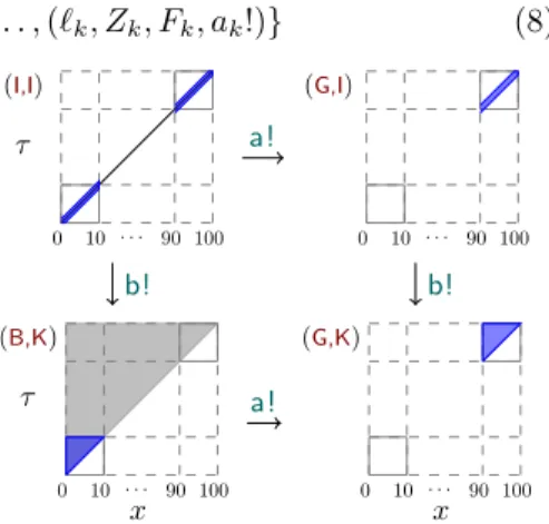
R: S = {(ℓ0, Z0, F0, a0!), . . . , (ℓk, Zk, Fk, ak!)} (8) (I,I) 0 10 · · · 90 100 τ (G,I) 0 10 · · · 90 100 (B,K) 0 10 · · · 90 100 x τ (G,K) 0 10 · · · 90 100 x a! b! a! b!
Fig. 3: Running example reachability set
R (grey) and strategy set S (blue) for
goalG∧ τ ≤ 100. where Fi ⊆ Zi and whenever vi ∈ Fi
then (ℓi, vi) ai!
−−→→∗ G. Also, (ℓ i, Zi)∈
R whenever (ℓi, Zi, Fi, ai!)∈ S. Thus, the union of the symbolic states (ℓi, Fi) appearing in quadruples ofS 4 identifies exactly the reachable states from which a discrete action ai! guar-antees to enter a good end of the timed automaton (or network). Fig. 3 depicts the reachability set R (grey area) and strategy set S (blue area) of our running example.
Given the strategy set S (8) and a state s = (ℓ, v), the set of possible delays after which an output action a! leads to a good end is given by
Dela!(s) ={ d | ∃(ℓi, Zi, Fi, a!)∈ S s.t. [s]d∈ Fi)}. For a single stochastic timed automaton DelG(s) =
∪
a!∈Σ!Dela!(s) and for a network DelG,i(s) =
∪ a!∈Σi
! Dela!(s). Importantly, note that Dela!((ℓ, v)) – and
thus also DelG((ℓ, v)) – can be represented as a finite union of disjoint intervals.
Given a closed zone Z and a valuation v, the Uppaal DBM library5 provides
functions that return the minimal delay (dmin) for entering a zone as well as the maximal delay for leaving it again (dmax). Due to convexity of zones then
{(v + d) | dmin≤ d ≤ dmax} ⊆ Z and thus the possible delays to stay in Z from 4
one symbolic state may appear in several quadruples.
5
v is equal to the interval [dmin, dmax]. For the remainder of this paper we write
{I1, I2. . . , In} = DelG(s) where I1, I2. . . In are the intervals making up DelG(s).
Extracting the possible actions from a state s = (ℓi, vi) after a delay of d is simply a matter of iterating over all elements (ℓi, Zi, Fi, ai!) inS and checking whether [s]d ∈ F
i. Formally, given a state s = (ℓi, vi), ActG,d((s)) ={ai!∈ Σ! | ∃(ℓi, Zi, Fi, ai!)∈ S s.t. [s]d ∈ Fi}.
5.2 On-the-fly State-wise Change of Measure
Having found methods for extracting the sets ActG,d(s) and DelG,k(s), we focus
on how to perform the state-wise change of measure.
Single Stochastic Timed Automaton In the following let A be a timed
automaton,TA= (L, δA•γA) be its stochastic timed transition system and let G be the goal states. For a fixed t obtaining samples ˜γA(s)(t) is a straightforward normalised weighted choice. Sampling delays from ˜δA(s) requires a bit more work: letI = {I1, I2, . . . In} = DelG(s) and let t∈ Ij, for some j then
˜ δA(s)(t) = ∫ δA(s)(t) τ∈DelG(s)δA(s)(t) dτ = ∫ τ∈IjδA(s)(t) dτ ∑ I∈I ∫ τ∈IδA(s)(τ ) dτ ·∫ δA(s)(t) τ∈IjδA(s)(t) dτ .
Thus, to sample a delay we first choose an interval–weighted by its probability– and then sample from the conditional probability distribution of being inside that interval. Since δA(s) is either an exponential distribution or uniform, integrating over it is easy and sampling from the conditional distribution is straightforward.
Network of Stochastic Timed Automata In the following letA1,A2, . . . ,An
be timed automata,Ti= (Li, δi•γi) be their stochastic timed transition systems and letJ = (J , ν) be their composition. Recall from previously we wish to ob-tain ˜υ∗(s)(t, a!) = κ δ k(s[k])(t) ∑n i=1( ∫ t′∈DelG,i (s)κ δ i(s[i])(t′) dt′) · κγ
k(s[k])(t, a!) for t ∈ DelG,k(s).
Let Ii = {Ii
1, I2i, . . . , Iki} = DelG,i(s) for all 1 ≤ i ≤ n and let t ∈ I for some I∈ Iw then ˜ υ∗(s)(t, a!) = ∫ Iκ δ w(s[w])(τ ) dτ ∑n i=1 ∑ I′∈Ii ∫ I′κ δ i(s[i])(τ ) dτ κδ w(s[w])(t) ∫ Iκ δ w(s[w])(τ ) dτ · κγ w(s[w])(t, a!),
when t∈ I and thus sampling from ˜υ∗ reduces to selecting an interval I and winner w, sample a delay t from ∫ κδw(s[m])(t)
Iκ δ
w(s[w])(τ ) dτ
and finally sample an action a! from κγ
w(s[w])(t, a!).
Algorithm 1 is our importance sampling algorithm for a composition of STA. In line 5 the delay densities of components according to standard semantics is extracted, and the win-densities (κδi) of each component winning is defined in line 6. In line 7 the delay intervals we should alter the distributions of κδi into is found. Lines 8 and 9 find a winning component ,w, and an interval in which
it won, and then lines 10 and 11 sample a delay from that interval according to
κδw. After sampling a delay, lines 13 and 14 sample an action. Afterwards the current state and likelihood ratio (L) is updated. The sampling in line 14 is a standard weighted choice, likewise is the sampling in line 9 - provided we have first calculated the integrals over κδi for all i. In line 11 the sampling from the conditional distribution is performed by Inverse Transform Sampling, requiring integration of κδk(s[k]).
Algorithm 1: Importance Sampling for Composition of STA Data: Stochastic Timed Automata:A1|A2| . . . |An
Data: Goal States: G
1 Let (L, δAi• γA1) =T
Ai for all i;
2 sc= initial state ;
3 L = 1 ;
4 while sc∈ G do/
5 Let δi= δAi(sc[i]) for all i;
6 Let κδi(t) = δi(t)· ∏ j̸=i (∫ τ >tδj(τ ) dτ ) for all i;
7 LetIi={I1, I2, . . . , In} = DelG,i(sc)for all i;
8 K(I, w) = ∫ Iκδw(t) dt ∑n i=1 ∑ I′∈Ii ∫ I′κ δ i(τ ) dτ for I∈ Im; 9 (I, w)∼ K ; 10 d(T ) = ∫ κδw(T ) Iκ δ w(τ ) dτ for T ∈ I; 11 t∼ d; 12 γ = γAw(s)(t); 13 m(a!) =∑ γ(a!) b!∈ActG,t(s)∩Σi! γ(b!) for a!∈ ActG,t(s)∩ Σi!; 14 a!∼ m; 15 sc= [[sc]t]a!; 16 L = L· δi(t)
K(I,w)·d(t)·m(a!)γ(a!);
17 return L;
A recurring requirement for the algorithm is thus that κδk(s[k]) is integrable: In the following we assume, without loss of generality, that s is a state where there exists some k such that for all i ≤ k, δi(s[i]) is a uniform distribution between ai and bi and for all i > k that δi(s[i])(t) = λie−λi(t−di) for t > di i.e.
δi(s[i]) is a shifted exponential distribution. For any i≤ k we can now derive that κδi(s[i])(t) = δi(s[i])(t)
∏ j̸=i (∫ τ >tδj(s[j])(τ dτ ) ) is 1 bi− ai ∏ j≤k,j̸=i bj−t bj−aj if aj≤ t ≤ bj 1 if t < aj 0 if bj < t or t < ai or t > ai · ∏ j>k ({ e−λi(t−di) if t > d i 1 else )
and in general it can be seen that κδi(s[i])(t) = P0(t)· E0(t) if t∈ I0 P1(t)· E1(t) if t∈ I1 .. . Pk(t)· Ek(t) if t∈ Il where I0, I1. . . Il are disjoint intervals covering [ai, bi], and for all j,Pj(t) is a polynomial constructed by the multiplication of uniform distribution andEj(t) is an exponential function of the form eα·t+β constructed by multiplying shifted exponential distributions. Notice that although we assumed i≤ k, the above gen-eralisation also holds for i > k. As a result we need to show for any polynomial,
P(t), that P(t) · eα·t+β is integrable.
Lemma 4 (6). LetP(t) =∑ni=0aiti be a polynomial and let E0(t) = eα·t+β be an exponential function with α, β∈ R≥0. Then ∫P(t) · E(t) dt = ˆP(t) · E(t), with
ˆ
P(t) =∑n+1 i=0 bit
i, where b
n+1= 0 and bi=ai−bi+1α(i+1). ⊓⊔
6
Experiments
In this section we compare the variance of our importance sampling (IS) estima-tor with that of standard SMC. We include a variety of scalable models,6 with
both rare and not-so-rare properties to compare performance. Running is a parametrised version of our running example. Race is based on a simple race between automata. Both Running and Race are parametrised by scale, which affects the bounds in guards and invariants. Race considers the property of reach-ing goal locationObs.Gwithin a fixed time, denoted♢≤1Obs.G. Running consid-ers the property of reaching goal location A.G within a time related to scale, denoted ♢≤scale·100A.G. The DPA (Duration Probabilistic Automata) are job-scheduling models [7] that have proven challenging to analyse in other contexts [12]. We consider the probability of all processes completing their tasks within parametrised time limit τ . The property has the form♢≤τDPA1.G∧ · · · ∧DPAn.G, whereDPA1.G, . . . ,DPAn.Gare the goal states of the n components that comprise the model.
The variance of our IS estimator is typically lower than that of SMC, but SMC simulations are generally quicker. IS also incurs additional set-up and initial analysis with respect to SMC. To make a valid comparison we therefore consider the amount of variance reduction after a fixed amount of CPU time. For each ap-proach and model instance we calculate results based on 30 CPU-time-bounded experiments, where individual experiments estimate the probability of the prop-erty and the variance of the estimator after 1 second. This time is sufficient to generate good estimates with IS, while SMC may produce no successful traces. Using an estimate of the expected number of SMC traces after 1 second, we are nevertheless able to make a valid comparison, as described below.
Our results are given in Table 1. The Gain column gives an estimate of the true performance improvement of IS by approximating the ratio (variance of
6
SMC estimator)/(variance of IS estimator) after 1 second of CPU time. The variance of the IS estimator is estimated directly from the empirical distribution of all IS samples. The variance of the SMC estimator is estimated by ˆp(1−
ˆ
p)/NSMC, where ˆp is our best estimate of the true probability (the true value
itself or the mean of the IS estimates) and NSMCis the mean number of standard
SMC simulations observed after 1 second.
For each model type we see that computational gain increases with rarity and that real gains of several orders of magnitude are possible. We also include model instances where the gain is approximately 1, to give an idea of the largest probability where IS is worthwhile. Memory usage is approximately constant over all models for SMC and approximately constant within a model type for IS. The memory required for the reachability graph is a potential limiting factor of our IS approach, although this is not evident in our chosen examples.
Param. Estimated Prob. IS Mem. (MB)
Model scale / τ P SMC IS σc2
is Gain SMC IS
Running
scale = 1 1.0e−1 1.0e−1 1.0e−1 2.5e−3 1.6 10.2 14.0 10 1.0e−2 1.0e−2 1.0e−2 2.5e−5 1.7e1 10.4 13.6 100 1.0e−3 1.0e−3 9.6e−4 2.5e−7 1.4e2 10.2 13.7
Race
1 1.0e−5 1.3e−5 1.6e−5 2.1e−11 8.3e3 10.0 13.5 2 3.0e−6 1.6e−6 3.2e−6 1.3e−12 2.0e4 10.0 13.3 3 1.0e−6 0 1.4e−6 2.5e−13 6.8e4 10.0 13.6 4 8.0e−7 0 8.0e−7 8.1e−14 1.5e4 11.5 14.4 DPA1S3
τ = 200 n/a 1.4e−1 1.4e−1 2.8e−2 1.1 10.2 11.9
40 n/a 3.6e−4 3.5e−4 1.7e−7 2.8e2 10.2 12.0
16 n/a 0 2.2e−8 6.9e−16 2.7e6 10.2 11.8
DPA2S6
423 n/a 1.0e−5 2.9e−5 3.7e−7 0.9 10.2 13.5
400 n/a 2.7e−5 7.6e−6 2.8e−8 3.0 10.3 13.5
350 n/a 0 5.5e−8 4.9e−13 1.1e3 10.3 13.3
DPA4S3
395 n/a 7.0e−5 1.9e−5 4.9e−8 4.4 10.3 53.1
350 n/a 1.4e−5 9.0e−6 1.3e−8 7.1 10.5 53.1
300 n/a 0 2.7e−7 2.3e−11 1.1e2 10.4 53.0
Table 1: Experimental Results.P is exact probability, when available. SMC (IS) indicates crude Monte Carlo (importance sampling). cσ2
is is empirical variance of
likelihood ratio. Gain estimates true improvement of IS at 1 second CPU time. Mem. reports memory use. Model DPAxSy contains x processes and y tasks.
7
Conclusion
Our approach is guaranteed to reduce estimator variance, but it incurs addi-tional storage and simulation costs. We have nevertheless demonstrated that our framework can make substantial real reductions in computational effort when estimating the probability of rare properties of stochastic timed automata. Com-putational gain tends to increase with rarity, hence we observe marginal cases
where the performance of IS and SMC are similar. We hypothesise that it may be possible to make further improvements in performance by applying cross-entropy optimisation to the discrete transitions of the reachability graph, along the lines of [9], making our techniques more efficient and useful for less-rare properties.
Importance splitting [11, 15] is an alternative variance reduction technique with potential advantages for SMC [10]. We therefore intend to compare our current framework with an implementation of importance splitting for stochastic timed automata, applying both to substantial case studies.
Acknowledgements
This research has received funding from the Sino-Danish Basic Research Centre, IDEA4CPS, funded by the Danish National Research Foundation and the Na-tional Science Foundation, China, the Innovation Fund Denmark centre DiCyPS, as well as the ERC Advanced Grant LASSO. Other funding has been provided by the Self Energy-Supporting Autonomous Computation (SENSATION) and Collective Adaptive Systems Synthesis with Non-zero-sum Games (CASSTING) European FP7-ICT projects, and the Embedded Multi-Core systems for Mixed Criticality (EMC2) ARTEMIS project.
References
[1] R. Alur and D. L. Dill. A theory of timed automata. Theor. Comput. Sci., 126(2):183–235, 1994.
[2] G. Behrmann, A. Cougnard, A. David, E. Fleury, K. G. Larsen, and D. Lime. Uppaal-tiga: Time for playing games! In 19th Int. Conf. on Computer Aided
Verification (CAV), pages 121–125, 2007.
[3] P. E. Bulychev, A. David, K. G. Larsen, A. Legay, G. Li, and D. B. Poulsen. Rewrite-based statistical model checking of wmtl. In RV, volume 7687 of
LNCS, pages 260–275, 2012.
[4] P. E. Bulychev, A. David, K. G. Larsen, A. Legay, G. Li, D. B. Poulsen, and A. Stainer. Monitor-based statistical model checking for weighted metric temporal logic. In LPAR, volume 7180 of LNCS, pages 168–182, 2012. [5] P. E. Bulychev, A. David, K. G. Larsen, A. Legay, M. Mikuˇcionis, and D. B.
Poulsen. Checking and distributing statistical model checking. In NASA
Formal Methods, volume 7226 of LNCS, pages 449–463. Springer, 2012.
[6] A. David, K. G. Larsen, A. Legay, U. Nyman, and A. Wasowski. Timed i/o automata: a complete specification theory for real-time systems. In HSCC, pages 91–100. ACM, 2010.
[7] A. David, K. G. Larsen, A. Legay, M. Mikuˇcionis, D. B. Poulsen, J. V. Vliet, and Z. Wang. Statistical model checking for networks of priced timed automata. In FORMATS, LNCS, pages 80–96. Springer, 2011.
[8] D. L. Dill. Timing assumptions and verification of finite-state concurrent systems. In Automatic Verification Methods for Finite State Systems,
Inter-national Workshop, Grenoble, France, June 12-14, 1989, Proceedings, pages
[9] C. Jegourel, A. Legay, and S. Sedwards. Cross-entropy optimisation of importance sampling parameters for statistical model checking. In P. Mad-husudan and S. A. Seshia, editors, Computer Aided Verification, volume 7358 of LNCS, pages 327–342. Springer, 2012.
[10] C. Jegourel, A. Legay, and S. Sedwards. Importance splitting for statistical model checking rare properties. In Computer Aided Verification, volume 8044 of LNCS, pages 576–591. Springer, 2013.
[11] H. Kahn. Use of different Monte Carlo sampling techniques. Technical Report P-766, Rand Corporation, November 1955.
[12] J. Kempf, M. Bozga, and O. Maler. Performance evaluation of schedulers in a probabilistic setting. In 9th International Conference on Formal Modeling
and Analysis of Timed Systems (FORMATS), pages 1–17, 2011.
[13] K. G. Larsen, P. Pettersson, and W. Yi. Uppaal in a nutshell. STTT, 1 (1-2):134–152, 1997.
[14] O. Maler, K. G. Larsen, and B. H. Krogh. On zone-based analysis of du-ration probabilistic automata. In Proceedings 12th International Workshop
on Verification of Infinite-State Systems (INFINITY), pages 33–46, 2010.
[15] G. Rubino and B. Tuffin. Rare Event Simulation using Monte Carlo
Meth-ods. Wiley, 2009.
[16] R. Rubinstein. The cross-entropy method for combinatorial and continuous optimization. Methodology And Computing In Applied Probability, 1(2):127– 190, 1999.
[17] E. Vicario, L. Sassoli, and L. Carnevali. Using stochastic state classes in quantitative evaluation of dense-time reactive systems. IEEE Transactions
on Software Engineering, 35(5):703–719, Sept 2009.
[18] H. L. S. Younes. Verification and Planning for Stochastic Processes with
Asynchronous Events. PhD thesis, Carnegie Mellon University, 2005.
[19] P. Zuliani, C. Baier, and E. M. Clarke. Rare-event verification for stochastic hybrid systems. In Proceedings of the 15th ACM International Conference